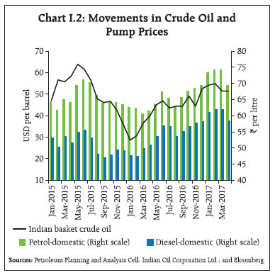
| I. Macroeconomic Outlook Underneath current benign inflation conditions, there are broad-based inflation pressures, which make the inflation outlook for 2017-18 challenging. Growth in real gross value added is expected to accelerate in 2017-18, underpinned by strong consumption demand even as investment activity remains muted and external demand uncertain. Under the monetary policy framework ushered in by amendments to the Reserve Bank of India (RBI) Act, the monetary policy decision has been vested in a six member monetary policy committee (MPC). Following its decision to lower the policy repo rate by 25 basis points (bps) at the time of the October 2016 Monetary Policy Report (MPR), the MPC decided to hold the policy rate in the December 2016 and February 2017 meetings of its bi-monthly schedule. Four features distinguish these initial decisions under the new regime. First, there was a calibrated shift in the policy stance from accommodative to neutral. Second, there was an overwhelming preference for waiting out the transitory effects of demonetisation and the unsettled political climate globally. Third, each decision was taken by unanimity. Fourth, within the consensus, members’ decisions appear to have been driven by individualistic approaches to arriving at them, as revealed in their written public statements. The recent experience of MPCs in the UK, Sweden, Brazil, Thailand, Czech Republic and Hungary suggests that rate decisions have been based on unanimity (Chart I.1). Other recent cases in point are the decisions of the US Federal Open Market Committee (FOMC) in its December 2016 and February 2017 meetings, and the Bank of England’s MPC in its meetings during October-February. Differences have been typically confined to the size of the change in the policy rate rather than contesting the overarching policy stance.1 Existing research on monetary policy decision making suggests that divergences stem mainly from (i) MPC members’ policy preferences – the relative weight on price stability and output stabilisation – in their reaction functions, and (ii) assessment of expected economic conditions – the evolution of inflation and output gaps.2,3 Does the formative experience of the MPC in India suggest similar policy preferences and assessments of the outlook? It is too early to tell. 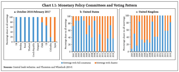 The analysis of macroeconomic developments presented in chapters II and III explains why both inflation and output growth have undershot the forecasts set out in the October 2016 MPR. In part, these deviations reflect the impact of demonetisation. Turning to the outlook, recent domestic and global events warrant revisions to the baseline assumptions on initial conditions set out in the October 2016 MPR (Table I.1). First, international crude oil prices have fluctuated widely over the last six months, hardening initially on the back of the agreement by Organisation of the Petroleum Exporting Countries (OPEC) to curtail production becoming credible.4 More recently, these prices have eased with shale production stepping up, US inventories rising sizeably and a vast amount of past supply.5 Nonetheless, oil prices are now ruling around 10 per cent above the level (US$ 46 per barrel) assumed in October 2016. Domestic petrol and diesel prices increased by around ₹5.5 per litre and ₹4.2 per litre, respectively, between November 2016 and February 2017 and were cut by around ₹4.9 per litre and ₹3.5 per litre, respectively, effective April 1, 2017 (Chart I.2). | Table I.1: Baseline Assumptions for Near-Term Projections | | Variable | October 2016 MPR | Current (April 2017) MPR | | Crude oil (Indian basket) | US$ 46 per barrel during FY 2016-17:H2 | US$ 50 per barrel during FY 2017-18 | | Exchange rate | ₹67/US$ | Current level | | Monsoon | Normal for 2016 | Normal for 2017 | | Global growth | 3.1 per cent in 2016
3.4 per cent in 2017 | 3.4 per cent in 2017
3.6 per cent in 2018 | | Fiscal deficit | To remain within BE 2016-17 (3.5 per cent) | To remain within BE 2017-18 (3.2 per cent) | | Domestic macroeconomic/ structural policies during the forecast period | No major change | No major change | Notes: 1. Crude oil (Indian basket) represents a derived basket comprising sour grade (Oman and Dubai average) and sweet grade (Brent) crude oil processed in Indian refineries in the ratio of 71:29.
2. The exchange rate path assumed here is for the purpose of generating RBI staff’s baseline growth and inflation projections and does not indicate any ‘view’ on the level of the exchange rate. The Reserve Bank is guided by the need to contain undue volatility in the foreign exchange market and not by any specific level/band around the exchange rate.
3. Global growth projections are based on July 2016 and January 2017 updates of the IMF’s World Economic Outlook.
4. BE: Budget Estimates. |
 Second, the foreign exchange market has experienced bouts of volatility triggered by international developments. The Indian rupee depreciated sharply vis-à-vis the US dollar during November 8-28, 2016 in the aftermath of the US presidential election results. Since then, the rupee has recovered lost ground and appreciated beyond the October 2016 level (₹67 per USD). Third, global growth and trade have evolved at a sluggish pace, as expected. Looking ahead, their pace is expected to accelerate modestly in 2017, benefitting from the expected fiscal stimulus in the US and the strengthening recovery from recent macroeconomic strains in major emerging market and developing economies (EMDEs). A sobering thought, however, is that global growth has repeatedly disappointed initial expectations in the past few years (Chart I.3). Consequently, downside risks suffuse the domestic outlook for 2017-18. I.1 The Outlook for Inflation Headline inflation declined to significantly low levels during November 2016-February 2017, much lower than projected in the October 2016 MPR. Yet, the persistence of inflation excluding food and fuel poses a challenge to the inflation outlook. Also, there is considerable uncertainty as to how prices will pan out over the coming months. As vegetable price declines were likely on account of demonetisationdriven distress sales in addition to seasonal factors,6 remonetisation could fuel a sharp reversal in vegetable prices, going forward. This development imparts uncertainty to the near-term outlook for inflation. 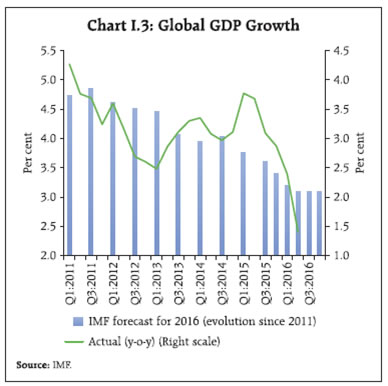 Households largely form inflation expectations adaptively, based on past movements in salient prices, especially those of food and fuel. The March 2017 round of the Reserve Bank’s survey of urban households indicated an increase of 20-50 bps in inflation expectations over the December round, reversing partly the sharp decline of 2-3 percentage points recorded in the previous (i.e., December) round. Three months and one year ahead inflation expectations were 7.5 per cent and 8.8 per cent, respectively. The proportion of respondents expecting the general price level to increase by more than the current rate also edged higher (Chart I.4). 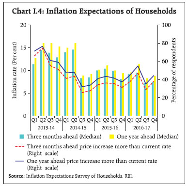 The hardening of global oil, metal and other commodity prices that is driving the recent surge in India’s wholesale inflation is imparting input price pressures for firms. Pricing power is also expected to improve, as reflected by manufacturing firms surveyed in the Reserve Bank’s industrial outlook survey in its January-March 2017 round (Chart I.5). Staff costs in the manufacturing sector are also expected to increase in Q1:2017-18. Nominal wage growth in rural areas decelerated in December- January, partly on account of demonetisation. Manufacturing and services sector firms in Nikkei’s purchasing managers’ survey for March 2017 reported pressures from both input prices and output prices. 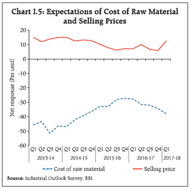 Professional forecasters surveyed by the Reserve Bank in March 2017 expected CPI inflation to pick up from its current level to 5.3 per cent by Q4:2017-18 (Chart I.6). Their medium-term inflation expectations (five years ahead) increased marginally by 10 bps to 4.8 per cent. Their longer-term inflation expectations (10 years ahead) remained unchanged at 4.5 per cent, close to the Reserve Bank’s medium-term inflation target of four per cent. 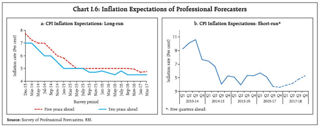 Taking into account the revised baseline assumptions, signals from the various forward-looking surveys and estimates from structural and other models (Box I.1), RBI staff’s baseline path for headline CPI inflation is expected to take it from its current level of 3.7 per cent (February 2017) to 4.2 per cent in Q1:2017-18, and 4.7 per cent in Q2. It is then forecast to edge higher to 5.1 per cent in Q3 on account of the demonetisationinduced base effect before moderating to 4.9 per cent in Q4:2017-18, with risks evenly balanced around this trajectory (the 50 per cent confidence interval for inflation in Q4:2017-18 is in a range of 3.4-6.4 per cent and the 70 per cent confidence interval is in a range of 2.6-7.2 per cent) (Chart I.7). Forecasts from the structural model indicate that inflation may evolve in a stable manner through 2018-19 and reach 4.6 per cent in Q4:2018-19 under the baseline scenario, with the monetary policy stance remaining unchanged. There are three major upside risks to the baseline inflation path – uncertainty in crude oil prices; exchange rate volatility due to global financial market developments, especially if political risks materialise; and implementation of the house rent allowances under the 7th Central Pay Commission (CPC) award. The likely impact of these shocks to headline inflation is explored in Section I.3. The proposed introduction of the goods and services tax (GST) in 2017-18 also poses some uncertainty for the baseline inflation path, particularly on account of oneoff but somewhat uncertain duration of price effects that are typically associated with the introduction of taxes on value added in the cross-country experience (see the October 2016 MPR for a review). Box I.1: Inflation Forecast Combinations Timely and reliable forecasts of inflation are critical inputs for setting forward-looking monetary policy. Forecasting inflation is challenging in all countries, both advanced and emerging, but it is rendered tenuous in emerging economies on account of recurrent supply shocks. Most central banks, therefore, use a suite of models, supplemented with informed judgement, for obtaining reasonably robust forecasts. Underlying this preference is a tacit recognition that all models are misspecified in some dimension and at some time points. In this context, a forecast combination approach – combining forecasts from alternative models through a judicious weighting system – finds favour among practitioners. Forecast combinations can act as a useful hedge against bad forecast performance of individual models, especially when inflation is volatile (Hubrich and Skudelny, 2017). In order to empirically validate if a forecast combination approach in the Indian context shows promising results vis-à-vis individual models, the following eight time series models are analysed: (i) a random walk (RW) model; (ii) a first-order autoregression (AR) model; (iii) a Phillips curve (PC) model; (iv) a moving average model with stochastic volatility (MA-SV); (v) a three-variable vector autoregression (VAR) model; (vi) a three-variable VAR with one exogenous variable (VARX) model; (vii) a Bayesian VAR (BVAR) model; and (viii) a Bayesian VARX (BVARX) model.7 Three approaches are used for combining the forecasts of the individual models: (i) a simple average of individual model forecasts; (ii) a performance-based weighted average, based on time varying weights (TVW) derived from the individual forecast performance of the past three years; and (iii) time varying geometrically backward decaying weights (TV-GDW) (i.e., a larger weight is given to the model’s recent performance). Quarterly data from Q1:2000 to Q3:2016 are used to estimate these models.  Forecast performance is measured by the inverse of the root mean square errors (RMSEs) of individual models and their combinations (relative to the benchmark RW model) for two alternative forecasting horizons (one quarter ahead and four quarters ahead) (Chart 1). The results suggest that (a) performance-based forecast combinations improve over both individual models and simple averaging; (b) the relative forecasting performance improves considerably as the horizon is extended from one quarter to four quarters, a feature especially helpful from the monetary policy perspective, given transmission lags. Overall, the results suggest that combining forecasts from a range of models outperforms an individual model. This is the approach that RBI staff adopts, as explained in the September 2015 MPR. Reference: Hubrich, K. and F. Skudelny (2017), “Forecast Combination for Euro Area Inflation: A Cure in Times of Crisis?”, Journal of Forecasting, DOI: 10.1002/for.2451. I.2 The Outlook for Growth With the effects of demonetisation turning out to be short-lived and modest relative to some doomsday expectations, the outlook for 2017-18 has been brightened considerably by a number of factors. First, with the accelerated pace of remonetisation, discretionary consumer spending held back by demonetisation is expected to have picked up from Q4:2016-17 and will gather momentum over several quarters ahead. The recovery will also likely be aided by the reduction in banks’ lending rates due to large inflows of current and savings accounts (CASA) deposits, although the fuller transmission impact might be impeded by stressed balance sheets of banks and the tepid demand for bank credit. Second, various proposals in the Union Budget 2017-18 are expected to be growth stimulating: stepping up of capital expenditure; boosting the rural economy and affordable housing; the planned roll-out of the GST; and steps to attract higher foreign direct investment (FDI) through initiatives like abolishing the Foreign Investment Promotion Board (FIPB). Third, global trade and output are expected to expand at a stronger pace in 2017 and 2018 than in recent years, easing the external demand constraint on domestic growth prospects. However, the recent increase in the global commodity prices, if sustained, could have a negative impact on our net commodity importing domestic economy. Finally, the pace of economic activity would critically hinge upon the outturn of the south-west monsoon, especially in view of the rising probability being assigned to an el niño event in July-August, 2017. Turning to forward-looking surveys, the consumer confidence moderated in the March 2017 round of Reserve Bank’s survey (Chart I.8). Respondents were less optimistic about the prospects for economic conditions, employment, and income a year ahead. Sentiment in the corporate sector improved during January-March 2017, according to the Reserve Bank’s industrial outlook survey (Chart I.9). The improvement was led by optimism on future production, order books, exports, employment, financial situation, selling prices and profit margin. Amounts mobilised through initial public offerings (IPOs) in recent months and filings of red herring prospectuses with the Securities and Exchange Board of India (SEBI) have been higher, which suggest investment optimism in the period ahead. Both manufacturing and services firms expected output to be higher a year from now, according to the purchasing managers’ survey for March 2017. Surveys conducted by other agencies indicate a decline in optimism over their previous rounds (Table I.2). 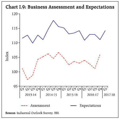
| Table I.2: Business Expectations Surveys | | Item | NCAER Business Confidence Index
(January 2017) | FICCI Overall Business Confidence Index
(January 2017) | Dun and Bradstreet Composite Business Optimism Index
(January 2017) | CII Business Confidence Index
(January 2017) | | Current level of the index | 112.0 | 58.2 | 65.4 | 56.5 | | Index as per previous Survey | 133.3 | 67.3 | 80.0 | 58.0 | | % change (q-o-q) sequential | -16.0 | -13.5 | -18.3 | -2.6 | | % change (y-o-y) | -14.0 | 2.6 | -23.9 | 4.8 | Professional forecasters surveyed by the Reserve Bank in March 2017 expected real GVA growth to accelerate from 6.5 per cent in Q4:2016-17 to 7.6 per cent in Q4:2017-18, led by growth in services and industry (Chart I.10 and Table I.3). 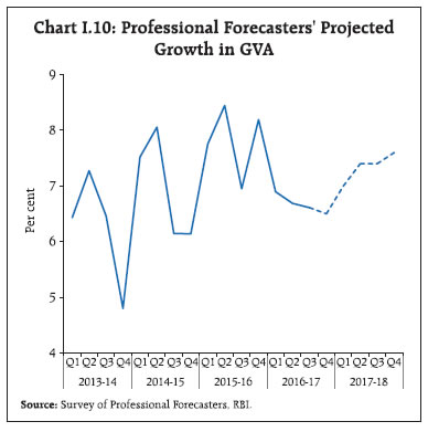
| Table I.3: Reserve Bank's Baseline and Professional Forecasters' Median Projections | | (Per cent) | | | 2016-17 | 2017-18 | 2018-19 | | Reserve Bank’s Baseline Projections | | | | | Inflation, Q4 (y-o-y) | 3.6 | 4.9 | 4.6 | | Real Gross Value Added (GVA) Growth | 6.7 | 7.4 | 8.1 | | Assessment of Survey of Professional Forecasters@ | | | | | Inflation, Q4 (y-o-y) | 3.6 | 5.3 | | | GVA Growth | 6.7 | 7.3 | | | Agriculture and Allied Activities | 4.2 | 3.5 | | | Industry | 6.1 | 7.0 | | | Services | 7.6 | 8.5 | | | Gross Domestic Saving (per cent of GNDI) | 31.5 | 31.8 | | | Gross Fixed Capital Formation (per cent of GDP) | 27.0 | 28.8 | | | Money Supply (M3) Growth | 7.5 | 10.5 | | | Credit Growth of Scheduled Commercial Banks | 6.0 | 10.0 | | | Combined Gross Fiscal Deficit (per cent of GDP) | 6.5 | 6.3 | | | Central Government Gross Fiscal Deficit (per cent of GDP) | 3.5 | 3.2 | | | Repo Rate (end period) | 6.25 | 6.00 | | | CRR (end period) | 4.00 | 4.00 | | | Yield of 91-day Treasury Bills (end period) | 6.0 | 6.3 | | | Yield of 10-year Central Government Securities (end period) | 6.8 | 6.7 | | | Overall Balance of Payments (US $ bn.) | 20.8 | 32.2 | | | Merchandise Exports Growth | 2.8 | 5.9 | | | Merchandise Imports Growth | -2.0 | 7.1 | | | Merchandise Trade Balance (per cent of GDP) | -5.0 | -5.1 | | | Current Account Balance (per cent of GDP) | -0.9 | -1.2 | | | Capital Account Balance (per cent of GDP) | 1.8 | 2.4 | | @: Median forecasts; GNDI: Gross National Disposable Income.
Sources: RBI staff estimates; and Survey of Professional Forecasters (March 2017). | Considering the baseline assumptions, the fast pace of remonetisation, survey indicators and updated model forecasts, RBI staff’s baseline scenario projects that real GVA growth will improve from 6.6 per cent in Q3:2016-17 and 6.5 per cent in Q4 to 7.0 per cent in Q1:2017-18 and 7.4-7.6 per cent in the remaining three quarters of 2017-18, with risks evenly balanced around this baseline path (Chart I.11). Looking beyond 2017-18 and assuming a normal monsoon, a congenial global environment, no policy induced structural change and no supply shocks, structural model estimates yield real GVA growth of 8.1 per cent in 2018-19. I.3 Balance of Risks The baseline projections of growth and inflation presented in the preceding section are based on the assumptions set out in Table I.1. As usual, there are uncertainties surrounding these assumptions which could produce deviations from baseline projections. This section assesses the sensitivity of the projected baseline paths of growth and inflation to plausible alternate scenarios. (i) International Crude Oil Prices The September 2016 announcement by OPEC of agreement on production cuts by members was met with scepticism. The signing of the agreement in end-November, however, led to a sharp jump in global crude oil prices. If OPEC sticks to the agreed production cuts of 1.2 mb/day till the next review of the agreement in May 2017, and the global crude oil production balance moves to a deficit by Q1:2017-18,8 upside risk to the crude oil trajectory over baseline estimates will heighten. Any supply disruptions due to geo-political developments could accentuate these upside risks. Assuming that crude prices increase to around US$ 60 per barrel under this scenario, inflation could be higher by around 30 bps and growth could be weaker by around 10 bps (Charts I.12 and I.13). 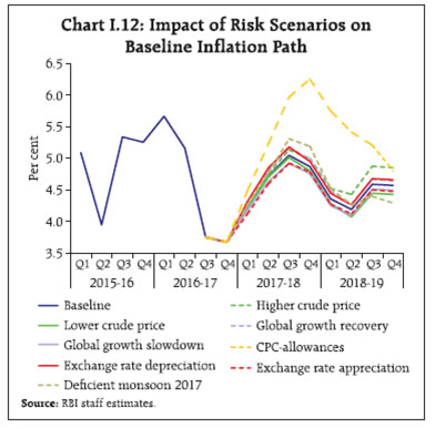 Conversely, if some of the OPEC members do not adhere to the agreed production cuts and/or the shale gas producers continue to ramp up production, global prices could soften below the baseline. Should crude prices slip under this scenario to around US$ 45 per barrel by 2017-18, inflation could moderate by around 15 bps with growth benefitting by around 5 bps. (ii) Global Demand The baseline scenario assumes that global growth will accelerate during 2017 and 2018. Risks to the baseline could emanate from: (a) US fiscal expansion being less than expected or marked by delays; (b) the Federal Reserve’s monetary policy response to expansionary fiscal policy being larger than expected, especially in the context of a recent assessment that the US economy is “closing in on full employment”; (c) the now pervasive spectre of protectionism affecting global trade; (d) continued concerns over the Chinese credit cycle; (e) volatile global crude oil and commodity prices; and (f) the implications of all these factors for international financial markets. Feedback loops can exaggerate the impact of several of these factors on global growth.9 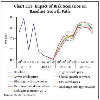 Assuming that global growth in 2017 and 2018 remains the same as was recorded in 2016 (i.e., 30-50 bps below the baseline assumption), real GVA growth and inflation could turn out to be around 20 bps and 10 bps, respectively, below the baseline. The pace of global economic activity could be higher if the policy stimulus in the US turns out to be larger than currently expected. In this scenario, assuming global growth is 50 bps higher, domestic growth could turn out to be around 25 bps above the baseline. Inflation could be higher by around 10 bps on the back of higher domestic demand as also imported impulses from higher global commodity prices. (iii) Seventh Central Pay Commission Allowances The 7th CPC recommended an increase in house rent allowance (HRA) of 8-24 per cent of basic pay. The higher HRA would have a direct and immediate impact on headline CPI through an increase in housing inflation. Assuming a rate of increase in the HRA as proposed by the 7th CPC is implemented from early 2017-18 onwards and the State Governments implement a similar order of increase with a lag of one quarter, CPI inflation could be 100-150 bps higher than the baseline for 2017-18.10 The HRA impact on inflation is expected to persist for 6-8 quarters, with the peak effect occurring around 3-4 quarters from implementation. In addition, indirect effects could occur from elevated inflation expectations. (iv) Exchange Rate Recognising that the domestic foreign exchange market witnessed heightened volatility in the aftermath of the US presidential elections, the risk of renewed turbulence in global financial markets on account of global downsides materialising and associated volatility in domestic financial markets remains a clear and present danger to the Indian economy. A five per cent depreciation of the Indian rupee, relative to the baseline assumption, could push up inflation by 10-15 bps in 2017-18. The depreciation, however, could have a favourable impact on growth in 2017-18 through a boost to net exports. In contrast, the combination of a benign global macroeconomic and financial environment, the expected acceleration in domestic growth and the policy initiatives to attract FDI flows can lead to an appreciation of the domestic currency, with a soothing impact on domestic inflation. A five per cent appreciation of the Indian rupee, relative to the baseline assumption, could soften inflation by 10-15 bps in 2017-18. (v) Deficient Monsoon Rainfall dependence of Indian agriculture makes the broader economy vulnerable to monsoon outcomes. The India Meteorological Department (IMD) is yet to release its forecast of the south-west monsoon for 2017. Hence, the baseline scenario assumes a normal south-west monsoon. However, the occurrence of el niño is assuming a rising probability, as stated earlier, dampening the prospects of agricultural production.11 Assuming the growth of output of agriculture and allied activities suffers by one percentage point, overall GVA growth could be lower by around 20 bps in 2017-18. The concomitant increase in food prices could result in headline inflation rising 30 bps above the baseline. To sum up, economic activity should recover in 2017- 18 on the back of the fast pace of remonetisation and the government’s focus on capital expenditure, rural economy and housing. The global economic environment may improve modestly, albeit amidst several uncertainties. Headline inflation is projected to increase during 2017-18, calling for close vigilance and readiness for an appropriate monetary policy response, if warranted.
II. Prices and Costs Consumer price inflation has eased significantly, mainly due to the large decline in food inflation, especially vegetables. Excluding food and fuel, however, inflation has remained sticky. Input costs have firmed up and pose upside risks to the path of inflation going forward. The MPR of October 2016 had projected CPI inflation1 moving in a narrow range of 5.0 to 5.3 per cent during Q3 and Q4 of 2016-17, on expectations of food inflation moderating and crude prices remaining benign. Food inflation came off its July 2016 peak and eased during August-October 2016. The shock of demonetisation, however, veered the inflation trajectory sharply below its projected path, essentially on account of an abrupt compression in food inflation. Prices of vegetables sank into deflation and pulled down headline inflation during November 2016-January 2017. Notwithstanding the hardening of global crude oil prices in the wake of the agreement on production cuts by OPEC in late November, the negative wedge between actual and projected inflation widened through the second half of 2016-17 (Chart II.1). II.1 Consumer Prices Headline inflation fell off its July cliff and was already traversing a declining trajectory during August through October when demonetisation hit in November. It triggered a downward spiral that took inflation down to 3.2 per cent in January 2017, an all-time low in the history of all India CPICombined (Chart II.2). The entire fall in inflation during November 2016 to January 2017 can be explained by the deflation in prices of vegetables and pulses. As a result, unfavourable base effects, which should have raised headline inflation during December 2016 to January 2017, were overwhelmed by a collapse in the month-on-month (m-o-m) momentum, bringing down headline inflation by around 100 basis points (Chart II.3). In February, however, the drag from these transitory effects began to ebb and headline inflation edged up on a pickup in food and fuel price pressures. 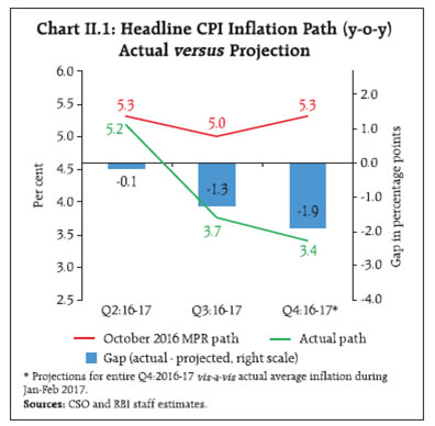 Despite the sharp fall in food inflation in the second half of the year, the distribution of inflation across all categories was largely centred around 4.5 per cent with continuing high kurtosis and a positive skew (Chart II.4). Diffusion indices for goods, services and the overall CPI were all well above 50 over the financial year, suggesting that even as headline inflation fell to a historic low, it was not broad-based (Chart II.5).
II.2 Drivers of Inflation In retrospect, a historical decomposition shows that it was the large shock delivered by demonetisation and the associated wage shock that explained much of the overall change in the inflation trajectory in the second half of 2016-17. Past monetary policy tightening continued to have visceral effects in containing inflation (Chart II.6a). In contrast, firmer crude prices and gradually closing output gap turned out to be sources of upside pressures, masked by the size of the demonetisation shock. Non-food inflation remained stubbornly sticky, hardened by the unchanging contribution of durable goods and services to overall inflation for much of the financial year (Chart II.6b). Inflation in the food and beverages category (with a weight of 46 per cent of CPI) turned out to be the active component of overall inflation in the second half of 2016-17.
Four factors stand out in the recent experience: First, prices of perishables played the most decisive role, even during the three months preceding demonetisation. In the months immediately following demonetisation, perishables became even more prominent, with vegetable price movements becoming pivotal after a decline of 21 per cent during November 2016 to February 2017. Transactions in fruits and vegetables have always been cash intensive. Anecdotal evidence points to distress sales by farmers, given their perishable nature. Vegetable prices usually do exhibit a seasonal moderation during November- February every year; during the 2016-17 season, however, the decline in vegetable prices was more pronounced than in previous years. Second, the vegetable prices decline troughed in January 2017 and thereafter showed a m-o-m increase of 0.1 per cent in February. Third, the seasonal decline in prices of vegetables is typically driven by potato, onion and tomato prices, which together constitute close to 40 per cent of the vegetables index. This time around, potato and tomato prices did exhibit seasonal easing but what was noteworthy was the plunge in the prices of other vegetables – cabbage, cauliflower, palak/other leafy vegetables, brinjal, gourd, peas and beans – which usually contribute little to the observed seasonality (Chart II.7). Fourth, inflation in perishables excluding vegetables averaged 5 per cent since November, considerably above the average headline inflation (Chart II.8).2 The spatial and temporal dynamics of food prices post-demonetisation show that within the food group, the decline in vegetable prices was particularly large and seen across states and across wholesale and retail markets (Box II.1). Excluding vegetables, food inflation would have been higher by 2.7 percentage points and headline inflation by 1.3 percentage points during November 2016 to January 2017. 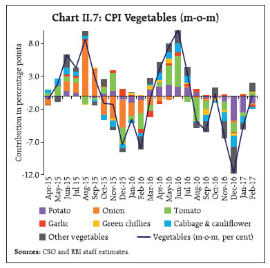 No commentary on inflation in the food and beverages category in the second half of 2016-17 would be complete without incorporating an analysis of the extraordinary developments in prices of pulses. With a weight of 5.2 per cent in the food group and only 2.4 per cent in the CPI, pulses contributed 13 per cent of the rising CPI inflation trajectory during the first half 2016-17. In the second half so far, prices of pulses turned into deflation and, with a contribution of (-) 2.5 per cent, aided in bringing down headline inflation to historic low in the CPI series. Inflation in arhar and urad, which had spiked pulses inflation during 2015-16 and the beginning of 2016-17, declined sharply during September 2016 to February 2017 so much so that arhar prices at the mandi level in the major producing states of Maharashtra, Madhya Pradesh, Gujarat and Karnataka dropped below the minimum support price (MSP). Gram prices, on the other hand, were an outlier, with inflation in this item rising dramatically before moderating in Q4:2016-17. After two consecutive years of production shortfall, adequate rainfall and better area coverage drove up pulses output during 2016-17 and mitigated price pressures considerably. Favourable supply side measures taken by the government such as imports at zero import duty3, extension in stock limit of pulses, raising MSPs in order to incentivise pulses production and maintaining buffer stocks also helped in reining in price pressures. 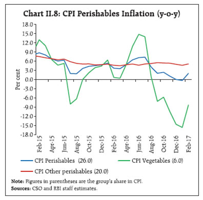 Box II.1: Anatomy of Food Deflation: Post Demonetisation State-wise CPI food inflation data for the period January 2013 to January 2017 were analysed at a monthly frequency in a panel framework in order to make a comparative assessment of spatial, temporal and intra-food group fixed effects in driving food inflation. Dynamic panel estimation1 was conducted on seasonally adjusted annualised m-o-m CPI food inflation. The results showed that while fixed effects were insignificant for most states, heterogeneity in inflation rates in sub-categories of food groups was significant. Even if the fiscal year 2016- 17 alone is considered, intra-food group fixed effects continued to remain significant for most groups. However, vegetables and pulses stood out in terms of magnitude and direction when compared with the usual patterns (Chart 1a and 1b). In the context of demonetisation, the panel analysis also showed significant time fixed effects for November 2016 brought about by vegetables, suggesting unusual decline in prices post demonetisation.  Furthermore, the fall in retail vegetable prices seemed to have broadly mirrored the fall in wholesale prices post demonetisation. Daily seasonally adjusted prices of potato and tomato, available for 88 centres across India, were used for analysing vegetable price margins post demonetisation (9 November - 31 December 2016), and remonetisation (January - February 2017). Using cluster analysis based on k-means clustering technique, the wholesale and retail prices were grouped into three major clusters – low, medium and high price clusters – based on the data of the pre-demonetisation period (September-October 2016). Post demonetisation, price moderation was observed across medium and high price clusters in the wholesale and retail markets. With progressive remonetisation, the prices in these vegetables started rising in both the wholesale and retail markets. The 45 degree line in Chart 2 represents the level where wholesale and retail prices are equal. In the case of tomato, retail prices fell even below wholesale prices for some centres, indicating a fall in retail margin post demonetisation. In the case of potato prices, the movement was mostly along and above the 45 degree line implying that margins were not impacted. The movement in margins* can also be seen from Chart 3. In the case of tomato, margins collapsed post demonetisation. As remonetisation progressed, margins rose again. These movements in margins were statistically significant**. In the case of potato, the analysis also showed that some centres experienced higher retail prices post demonetisation compared with wholesale prices, suggesting that in some cases the widening of retail-wholesale margins was centre-specific. 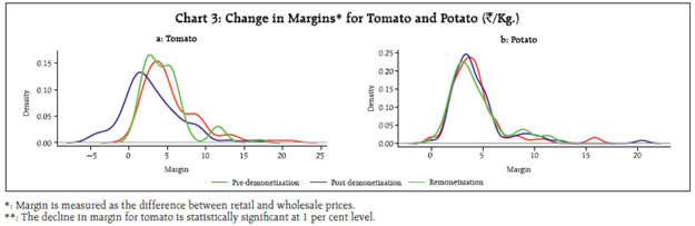 Within the food group, there were upside price pressure points in sugar, cereals and other food items such as prepared meals. Slippage in production during 2015-16 and 2016-17 caused double-digit inflation in sugar prices during the year (Chart II.9a and b). Under cereals, inflation in respect of rice has eased during October 2016 - January 2017, while inflation in wheat continued to firm up. A number of price control measures have been undertaken by the government for containing the price rise in the case of sugar and edible oil, including imposition of stockholding limits, discouraging exports, and reduction in import duty on certain edible oils. In the fuel group, the moderation in inflation in the first half of the financial year reversed and it picked up from December 2016, driven by LPG and kerosene. The rise in LPG broadly mirrored the turnaround in international LPG prices. In the case of kerosene, the uptick was driven by the increase in subsidised kerosene prices by a calibrated ₹0.25 per litre per month during July 2016 to February 2017, in addition to rising international prices. The weighted contribution of firewood and chips to overall fuel inflation remained broadly unchanged (Chart II.10), underscoring the persistence in fuel inflation across rural areas. CPI inflation excluding food and fuel remained sticky at around 5 per cent during most of the second half of 2016-17 (Chart II.11a). Housing and ‘clothing and footwear’ sub-groups were the main contributors, accounting for 36.2 per cent of inflation in the category as a whole. Other upside pressures in the group emanated from the firming up of international crude oil prices since December 2016 and the lagged pass-through to domestic prices of petrol and diesel that are embedded in transport and communication. With excise duty increase of around ₹12 per litre for both petrol and diesel under additional revenue mobilisation (ARM) measures, the mark-up of domestic over global prices has become more pronounced. With softening of international crude oil prices since early February 2017, domestic pump prices of petrol and diesel were reduced with a lag in the beginning of April 2017 (Chart II.12). 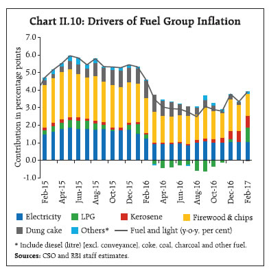 Excluding volatile components such as petrol and diesel, inflation in this group (CPI, excluding food and fuel) averaged 4.7 per cent between September 2016 and February 2017 (Chart II.11a). Some moderation in February came about on account of the goods component in this category – gold and silver in ‘personal care and effects’; pharmaceuticals in health; and garments in the clothing sub-groups – although more readings need to be monitored to assess whether this softening will endure (Chart II.13a). By contrast, the contribution of the services component in all these sub-groups remained sticky, especially housing and education services (Chart II.13b). Given the incidence of large and frequent supply shocks on food and non-food items, trimming the inflation distribution by removing specific portions of upper and lower tails of the distribution is widely used to assess underlying inflation movements, with the weighted median being a specific case of trimming. Trimmed means, the weighted median and exclusionbased measures of CPI inflation revealed a central tendency of 4.7 per cent during September 2016 to February 2017 (Chart II.11b). Notwithstanding some moderation in February, the downward inflexibility in inflation excluding food and fuel has infused significant upside risks into the near-term outlook. The direct and indirect impact on housing inflation of the 7th CPC house rent allowance award – once implemented by the Government – and the size and duration of the ‘GST effect’ are other upside risks to inflation in CPI in this category.
Other Measures of Inflation An important development in the second half of 2016-17 is the divergence that has set in between inflation measured by the CPI and by other measures. This conveys valuable insights into the profile of CPI inflation as it evolves in the months ahead. Inflation measured by the sectoral consumer price indices undershot headline CPI inflation, reflecting, inter alia, the higher weight of food in the former as also the absence of items such as gold and silver that were recent pressure points. Inflation in terms of the wholesale price index (WPI) was closely co-moving with CPI inflation during October-December 2016, but it shot up in January and further in February to close to three percentage points above CPI inflation, driven by a sharp pick-up in international commodity prices. GDP and GVA deflators rose in the beginning of the year, but edged down closer to CPI inflation from Q3:2016-17 (Chart II.14).
II.3 Costs Even as retail inflation and its measurement by other metrics has shrugged off the transitory drag of demonetisation and revealed its underlying trajectory in the February 2017 reading, cost push pressures appear to be coalescing. Domestic farm and non-farm input costs escalated significantly in the second half of 2016-17 on account of the rise in global crude oil prices, the firming up of metal prices and expectations of expansionary US fiscal spending (Chart II.15). 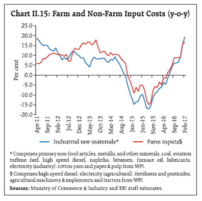 Coal inflation surged in January and February, with Coal India Limited linking its premium quality coal to international prices which hardened on account of supply disruptions in Australia and China towards the end of 2016. Substantial price pressures were also observed in high speed diesel, naphtha, furnace oil, cotton yarn and fibres all of which drove up inflation in industrial input costs to the highest level since early 2011. In the farm sector, price increases relating to high speed diesel and pesticides, particularly weedicides, largely contributed to the upturn in farm input costs. An analysis based on the Supply and Use Table (SUT) of the Central Statistics Office (CSO) comprising 140 products/services and 66 industries shows that a one per cent increase in crude oil, metals and coal prices could translate into an increase in WPI inflation by 15 bps, 20 bps and 5 bps, respectively, and in CPI inflation by 6 bps, 7 bps and 2 bps, respectively.4 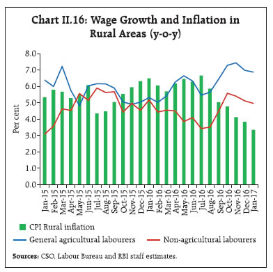 Turning to wages and staff costs, rural wage growth for both agricultural and non-agricultural labourers picked up through October-November 2016 before moderating in December and January (Chart II.16). The divergence between agricultural and non-agricultural wage growth remains wide, reflecting the increase in demand for farm labour due to the invigoration of agricultural activity. 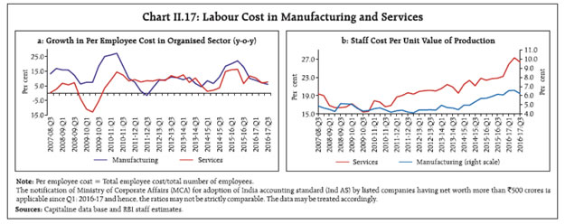 In the organised sector, corporate sector performance points to a moderation in per employee staff cost of listed private sector companies (Chart II.17a). A caveat in interpreting these developments is that the value of production grew at a slower pace than staff costs pushing up unit labour costs (i.e., the ratio of staff cost to value of production) for both manufacturing and services companies, notwithstanding the moderation seen in the latest reading (Chart II.17b). Firms polled in the Reserve Bank’s industrial outlook survey reported a sharp pick-up in the cost of raw materials as also in staff cost. Most of the firms expect to pass on the increase in costs into selling prices. Similar sentiments about acceleration in input costs were reported by both manufacturing firms and service providers in purchasing managers’ indices. Polled companies expect that the increase in costs will strengthen output price inflation. Going forward, the inflation path will be shaped by the implementation of house rent allowances under the 7th CPC award and the introduction of the GST; both these developments are likely to provide a push to headline inflation, the impact of which could last for 12-18 months. Moreover, several parts of the corporate sector, which have been struggling with balance sheet stress for a protracted period, await a recovery in demand that will rekindle pricing power of firms so that they can rebuild their bottom lines. While input costs have firmed up, the outlook for inflation will hinge upon a reasonably accurate assessment of the quantum of input price increases that the firms may pass through to their output prices. Further, should the recent softening in crude oil prices – caused by build-up in oil stocks in the US, legacy oversupply from OPEC last year, and possible failure of production controls by OPEC and Russia – continue, inflation trajectory could soften. Finally, with the rising probability of el niño, as discussed in Chapter 1, the path of food inflation may be impacted by the outcome of the monsoon in the coming year and in this regard, supply management measures that have successfully led to deceleration in food inflation from double digits in 2012-13 and 2013-14 to close to 5 per cent in 2016-17 so far, will play a crucial role.
III. Demand and Output The slowdown in aggregate demand, which set in at the beginning of H2:2015-16, became accentuated in H2: 2016-17, although consumption demand remained resilient. Aggregate supply conditions were underpinned by the robust performance of agriculture and steady government expenditure. Economic activity has been losing momentum since H2:2015-16 on a combination of structural and cyclical factors; in H2:2016-17, this trajectory was dented further by the transient impact of demonetisation. Both private and government consumption demand have held up well against this slowdown, together accounting for 90 per cent of real gross domestic product (GDP) growth in H2:2016-17 on a weighted contribution basis. Investment demand, which had sunk into contraction in H1, recovered from Q3:2016- 17. Net exports have been growing strongly since Q3:2015-16 but in Q3:2016-17, they turned negative with imports starting to expand at a higher pace than exports as domestic demand strengthened. The ebullient rebound in agricultural activity on the back of normal monsoon and record foodgrains production have boosted rural incomes and supported consumption. In contrast, the modest pick-up in industry in H2:2016-17 and the slower growth in services suggests that investment demand is still sluggish. Going forward, implementation of the Goods and Services Tax (GST) and the measures taken in the Union Budget to boost the rural economy, infrastructure, micro, small and medium enterprises (MSMEs) and low cost housing should help invigorate domestic demand. However, a sustained revival of investment holds the key to stepping up the pace of economic activity closer to its medium-term potential. III.1. Aggregate Demand Aggregate demand measured by y-o-y changes in real GDP at market prices moderated through 2016-17, with the slowdown being pronounced in the second half of the year. Fiscal stimulus in the form of the 7th Central Pay Commission’s (7th CPC) award supported aggregate demand strongly; without the support of government final consumption expenditure (GFCE), GDP growth would have slumped to 5.9 per cent in H2:2016-17 as against the headline print of 7.0 per cent1. Private consumption remained the mainstay of domestic demand, notwithstanding some deceleration expected in the last quarter of the year. On a seasonally adjusted basis, however, q-o-q growth suggests that the slowdown in aggregate demand bottomed out in Q3 and an upturn commenced in Q4 on the back of a tentative recovery in exports and investment (Chart III.1, Table III.1). III.1.1 Private Final Consumption Expenditure Private final consumption expenditure remains the bedrock of domestic demand, contributing over half of overall GDP growth in H2:2016-17 (Chart III.2). Its underlying resilience stood out in the face of cash constraints of demonetisation, with data pointing to an acceleration of growth in this period on a sequential basis. The expansion of consumer purchasing power in this period can be explained by a combination of factors: improved rural consumption demand due to (i) robust agricultural activity; (ii) sharp uptick in Mahatma Gandhi National Rural Employment Guarantee Act (MGNREGA) expenditure (15 per cent for 2016-17); and (iii) rural wages remaining steady; implementation of 7th CPC recommendations and One Rank One Pension (OROP) which buoyed already strong urban consumption demand and a significant fall in overall consumer inflation. 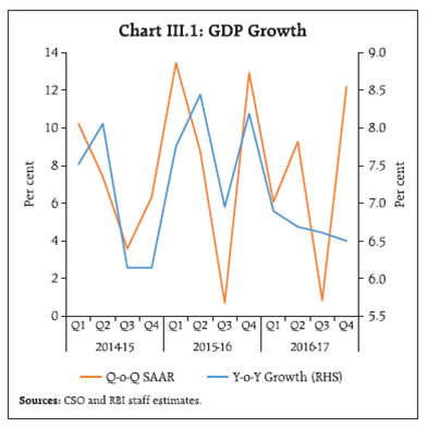
| Table III.1: Real GDP Growth | | (Per cent) | | Item | 2015-16 | 2016-17 (SAE) | Weighted contribution to growth in 2016-17 (percentage points)* | 2015-16 | 2016-17 | | Q1 | Q2 | Q3 | Q4 | Q1 | Q2 | Q3 | Q4# | | Private Final Consumption Expenditure | 7.3 | 7.2 | 4.0 | 4.9 | 6.7 | 6.8 | 10.6 | 7.2 | 5.1 | 10.1 | 6.5 | | Government Final Consumption Expenditure | 2.9 | 17.0 | 1.7 | 0.5 | 3.9 | 3.7 | 3.6 | 15.5 | 15.2 | 19.9 | 18.1 | | Gross Fixed Capital Formation | 6.1 | 0.6 | 0.2 | 9.6 | 12.4 | 3.2 | 0.0 | -2.2 | -5.3 | 3.5 | 6.5 | | Net Exports | 13.9 | 62.0 | 0.7 | -1.1 | -4.9 | 27.0 | 89.6 | 70.4 | 74.5 | -23.4 | - | | Exports | -5.4 | 2.3 | 0.5 | -5.7 | -4.3 | -9.0 | -2.5 | 2.1 | -0.9 | 3.4 | 4.4 | | Imports | -5.9 | -1.2 | -0.3 | -5.2 | -3.6 | -10.2 | -4.4 | -2.7 | -7.4 | 4.5 | 1.4 | | GDP at Market Prices | 7.9 | 7.1 | 7.1 | 7.8 | 8.4 | 6.9 | 8.6 | 7.2 | 7.4 | 7.0 | 7.0 | SAE: Second Advance Estimates. #: Implicit growth.
*: Component-wise contributions to growth do not add up to GDP growth in the table because change in stocks, valuables and discrepancies are not included.
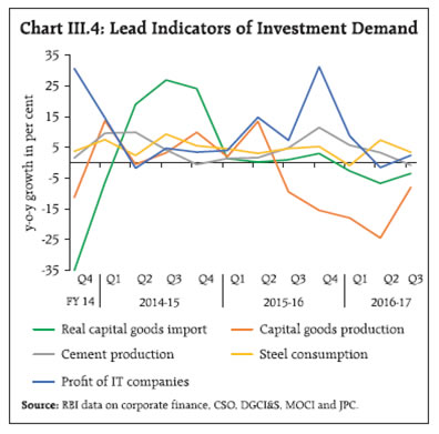
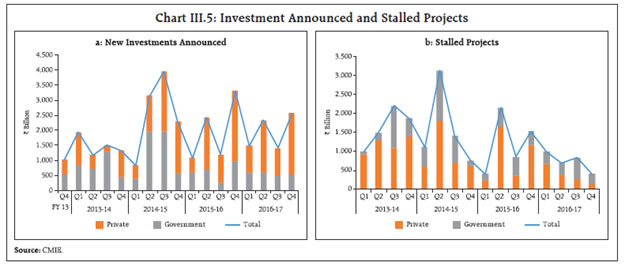
Source: Central Statistics Office (CSO). | In terms of lead indicators for estimating private final consumption expenditure, the surge in private consumption finds reflection in the acceleration in agriculture GVA, telephone connections, indirect tax collections and manufacturing index of industrial production (IIP) (Chart III.3). III.1.2 Gross Fixed Capital Formation After four consecutive quarters of either sharp deceleration or contraction, gross fixed capital formation turned around in Q3 and accelerated further in Q42. On the basis of lead indicators, this reversal in investment demand in spite of demonetisation effects can be explained by the pick-up in capital goods imports and moderation in the pace of contraction in domestic capital goods production as also improvement in profits of software companies (Chart III.4). Some momentum in investment activity is also visible in sectors such as electricity transmission, roads and renewable power. 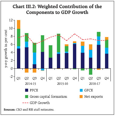 Nonetheless, it may be premature to interpret these proximate developments as green shoots of durable revival of investment demand. A wider scan shows that capex spending, especially in large brownfield projects in sectors such as iron and steel, construction, textiles and power, remains weak amidst an environment of uncertainty surrounding growth, both global and domestic, and over-indebtedness as well as excess capacity in many sectors. According to the Centre for Monitoring Indian Economy (CMIE), new investment proposals, which capture the future pace of investment activity, has recovered in Q4 from its decadal low level in Q3, driven by government projects. The new investment projects increased to ₹2.57 trillion in Q4 as against an average of ₹2.16 trillion in the preceding nine quarters (Chart III.5a). The value of stalled projects decreased by 51 per cent during the quarter, mainly accounted for by government sector projects (Chart III.5b). The problem of stalled projects continues mainly because of lack of environmental and non-environmental clearances. 
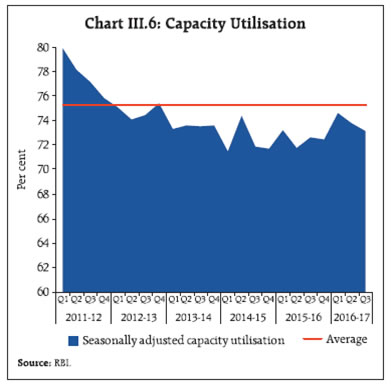 Seasonally adjusted capacity utilisation has remained below its average (since Q1:2013-14), reflecting weak demand and raising concerns on the sustainability of the recent pick-up in private investment (Chart III.6). Decomposition of time series into trend and cycles of various frequencies, juxtaposed with a Markov switching exercise to detect regime shifts also suggests that the recent upturn may not yet confirm a definitive reversal in investment demand (Box III.1). Going forward, an increase in allocation of capital expenditure by 10.7 per cent in the Union Budget 2017-18 is expected to generate some multiplier effects, but the catalytic effects of fiscal crowding in setting off a turnaround in the investment cycle is largely contingent on revival in private investment appetite. A binding constraint is the heightened risk aversion among banks, many laden with double-digit percentage of stressed assets to gross advances, to finance sectors that are excessively leveraged. Sectorspecific slack and demand substitution through cheaper imports in some segments due to excess global capacity are other drags on the revival in investment. Box III.1: Investment Cycle in India: Some Insights from Wavelet Analysis Gross domestic investment in India has been muted in a prolonged phase that set in during the post global financial crisis (GFC) period. Capacity utilisation has remained low and industrial activity depressed in an environment characterised by subdued global and domestic demand. Consequently, when gross fixed capital formation (GFCF) posted positive growth in Q3:2016-17 after three consecutive quarters of contraction, one question has evoked considerable interest: Is the recent upturn indicating a turning point in the investment cycle and what are the implications for growth? The Markov switching model of Hamilton (1989) was applied on growth rates (annualised seasonally adjusted q-o-q) of investment [chart (a)] to check whether the recent surge in the investment growth rate is, in fact, a turning point. Markov-switching probabilities suggest that the inflexion point in the investment cycle to a higher growth regime has still not materialised. Similar exercise on GDP growth rates [chart (b)] also does not suggest any turnaround. Furthermore, output and investment growth cycles (annualised q-o-q) are also examined using Wavelet analysis which offers the possibility of decomposing the time series data into several series of orthogonal sequences of scales representing different periodicities/ frequencies. Charts (c) and (d) present the wavelet transformation of GDP and GFCF growth rates [first panel in Charts (c) and (d)] into a low frequency scale that represents the long-run trend in the growth rates [second panel in Charts (c) and (d)] and four relatively higher frequency levels [third to sixth panel in Charts (c) and (d)]. The addition of these low frequency and high frequency decompositions produces the observed data. Long-term GDP and GFCF growth rates seem to have moderated in the years following the global financial crisis. The moderation in the long-term investment cycle has been much sharper than the output growth cycle. The lower frequency cycles (of periodicities 2-4 years) of output growth do not show any visible signs of a turnaround in the recent period. However, the investment cycle (of periodicity 2 years) indicates some increase [fourth panel in Chart (d)] consistent with the higher GFCF growth rates recorded in H2:2016-17. 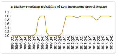
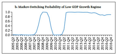
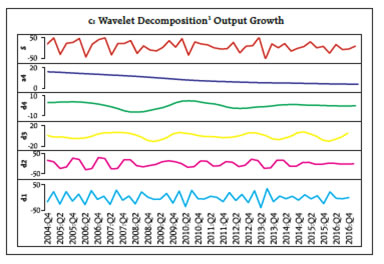

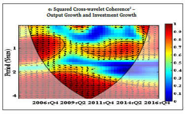 Notes: 1. Using Daubechies 4 wavelet at level 4 (Smooth wavelets like the Daubechies 4 give better approximations to continuous functions). The first panel in Charts(a) and (b) are the annualised q-o-q changes of GFCF and GDP, respectively – represented by S = a4 + d4 + d3 + d2 + d1. 2. Cross wavelet and wavelet coherence software were provided by A. Grinsted http://www.glaciology.net/wavelet-coherence. The Morlet family of wavelet is used, as it provides a good balance between time and frequency localization. Horizontal axis shows time, while vertical axis shows period in years. The warmer the colour of region (more red), the higher the degree of coherence between investment and output growth cycles. Arrows indicate the relative phase relationship between the series (pointing right: in-phase; left: anti-phase; up: GFCF leading GDP). Black thick contour represents 5 per cent significance. The red coloured regions inside the black thick contours of the cross wavelet coherence in Chart (e) represent the high and significant co-movement between output and investment cycles at different time points (in x-axis) and at different cycle lengths represented by period (in y-axis). This indicates that output and investment cycles strongly co-moved in the 2-4 year cycle during the pre-crisis period, but co-moved only in the 3-4 year cycle in the recent period. Therefore, the uptick in the 2-year period cycle for investment might not immediately translate into higher output growth. References: Hamilton, James D (1989), “A New Approach to the Economic Analysis of Nonstationary Time Series and Business Cycle”, Econometrica, March, 57(2). Yogo, M. (2008), “Measuring Business Cycles: A Wavelet Analysis of Economic Time Series”. Economics Letters, 100(2), pp. 208-212. III.1.3 Government Expenditure Another key component of aggregate demand - government final consumption expenditure (GFCE) - continued to provide strong support to aggregate demand in H2:2016-17 due to the implementation of the 7th CPC award and OROP. Lower spending on all major subsidies - food, fertilisers and petroleum - contained Central Government’s revenue expenditure at the budgeted level for 2016-17. Although there was a shortfall in realisation of budgeted receipts from disinvestment and spectrum auctions, buoyant indirect tax collections and non-tax revenues helped in realising the fiscal deficit target even as capital expenditure did not experience any cutbacks, unlike in previous years (Table III.2). In fact, the revised estimates (RE) of capital expenditure were 13.3 per cent higher than budgeted estimates (BE), reflecting improvement in expenditure quality. Union excise duty collections grew by 34.5 per cent on a y-o-y basis on account of the upward revision in clean environment cess, imposition of infrastructure cess on certain motor vehicles, additional excise duty on jewellery articles and increase in excise duty on tobacco products. Receipts from the service tax grew by 17.1 per cent due to imposition of Krishi Kalyan cess at 0.5 per cent from June 1, 2016. Relatively robust indirect tax collections and lower spending on subsidies also entailed a wider divergence between GVA and GDP growth rates. The Union Budget, 2017-18 deferred the target for the gross fiscal deficit (GFD) to GDP ratio of 3.0 per cent to 2018-19 from 2017-18. Nevertheless, the government remained committed to the spirit of fiscal consolidation as the Centre’s GFD is budgeted to decline by 0.3 percentage point to 3.2 per cent in 2017-18 through an increase in non-debt receipts, particularly tax revenues and disinvestment proceeds. This makes room for enhanced budgetary allocation for the farm and rural sectors, social and physical infrastructure, and employment generation. Future fiscal consolidation is contingent upon efficient revenue mobilisation - broadening the tax base; and incentivising digital payments. | Table III.2: Key Fiscal Indicators - Central Government Finances | | Item | Per cent to GDP | 2016-17
(BE) | 2016-17
(RE) | 2017-18
(BE) | | 1. Revenue Receipts | 7.9 | 9.3 | 9.0 | | a. Tax Revenue (Net) | 6.3 | 7.1 | 7.3 | | b. Non-Tax Revenue | 1.7 | 2.2 | 1.7 | | 2. Non Debt Capital Receipts | 0.4 | 0.4 | 0.5 | | 3. Revenue Expenditure | 11.5 | 11.4 | 10.9 | | 4. Capital Expenditure | 1.6 | 1.8 | 1.8 | | 5. Total Expenditure | 13.1 | 13.2 | 12.7 | | 6. Gross Fiscal Deficit | 3.5 | 3.5 | 3.2 | | 7. Revenue Deficit | 2.3 | 2.0 | 1.9 | | 8. Primary Deficit | 0.3 | 0.3 | 0.1 | Source: Union Budget, 2017-18.
Note: BE: Budget Esitmates RE: Revised Estimates |
| Table III.3: Major Deficit Indicators of State Governments | | (Per cent of GSDP) | | Item | 2016-17
(BE) | 2016-17
(RE) | 2017-18
(BE) | | Revenue Deficit | -0.1 | 0.2 | -0.1 | | Gross Fiscal Deficit | 3.0 | 3.4 | 2.6 | | Gross Fiscal Deficit ( Excluding UDAY) | - | 3.0 | - | | Primary Deficit | 1.3 | 1.7 | 0.9 | Notes: 1. Negative (-) sign indicates surplus.
2. Data pertain to 21 out of 29 States.
3. UDAY data as per RBI records.
Source: Budget Documents of State Governments. | The latest available data in respect of 21 States suggest an increase in GFD to gross state domestic product (GSDP) ratio to 3.4 per cent in 2016-17 (RE) against 3.0 per cent budgeted. Net of Ujwal DISCOM Assurance Yojana (UDAY) bonds, however, the ratio was lower at 3.0 per cent. For 2017-18 (BE), The GFD-GSDP ratio of 21 states works out to 2.6 per cent (Table III.3). The deterioration in State finances during 2016-17 will impact the overall fiscal position of the general government. The Centre’s borrowing programme was conducted as per the planned issuance schedule within the overall contour of debt management strategy. Combined gross market borrowings of the Centre and States (dated securities) during 2016-17 increased by 9.6 per cent over the previous year (Table III.4). Increased borrowing by the state governments may exert pressure on the finite pool of investible resources and crowd out private investment. | Table III.4: Government Market Borrowings | | (₹ billion) | | Item | 2015-16 | 2016- 17 | | Centre | States | Total | Centre | States | Total | | Net Borrowings | 4,406.3 | 2,611.9 | 7,018.2 | 4,082.0 | 3,426.5 | 7,508.5 | | Gross Borrowings | 5,850.0 | 2,945.6 | 8,795.6 | 5,820.0 | 3,819.8 | 9,639.8 | III.1.4 External Demand After making positive contribution to GDP in the last four quarters, net exports contracted sharply and pulled down GDP growth in Q3:2016-17. Growth in merchandise exports as well as imports turned positive for the first time in eight quarters; however, a stronger pick-up in imports than in exports expanded the trade deficit in Q3 and the first two months of Q4. Notwithstanding the slowdown in global demand, evident in weak imports by advanced economies (AEs), India’s exports to AEs resisted this slowdown and actually increased in Q2 and Q3:2016-17 alongside the pick-up in exports to emerging market economies (EMEs) which had accounted for a large part of the decline in India’s exports over the last two years. In fact, export shipments to EMEs registered positive growth for the first time since Q3:2014-15. Significantly, the turnaround in India’s export growth in Q3 was led by non-oil exports with almost the entire increase in oil exports accounted for by the increase in international crude oil prices. Exports of some labourintensive sectors such as ready-made garments, gems and jewellery, and leather and products experienced transient pressures from demonetisation. All broad categories of imports, viz. oil, gold and non-oil non-gold imports, increased during October-February 2016-17 (Chart III.7). Gold imports, which rose in November after demonetisation and declined sharply in the next two months, increased in February 2017 due to domestic stockpiling ahead of festive (Akshaya Tritiya) and wedding season. Strong price effects caused by Organisation of the Petroleum Exporting Countries (OPEC) production cut pushed up the growth of oil imports in nominal terms even as import volumes declined in recent months. 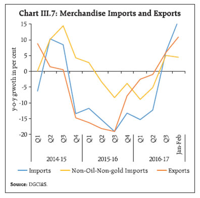 Net services exports moderated in H2:2016-17 (October 2016 - January 2017) in relation to the corresponding period of 2015-16. Among services exports, India’s software exports face uncertainty from global headwinds, especially from the likely restrictions relating to the H1-B visas. A higher flow of tourist arrivals augured well for exports of travel services. The net outgo due to investment income payments in Q3, however, was marginally lower than in the corresponding period of 2015-16. Private transfer receipts, mainly representing remittances by Indians employed overseas, declined by 3.8 per cent in Q3 from their level a year ago. Despite a lower merchandise trade deficit, current account deficit at 1.4 per cent of GDP in Q3 was almost at the same level as a year ago, though higher than the preceding two quarters. While net FDI inflows at US$ 13.2 billion in H2:2016- 17 (October 2016 - January 2017) moderated from the level a year ago, net portfolio flows turned positive in Q4. On a cumulative basis, net FDI inflows, however, rose to US$ 33.9 billion in April-January 2016-17 as compared with US$ 31.6 billion a year ago, suggesting India is becoming a preferred investment destination. The bout of global risk aversion that caused net outflow of foreign portfolio investment (FPI) during November 2016 to January 2017 subsided subsequently as foreign portfolio investors turned net buyers in response to the Union Budget proposals and the change in the monetary policy stance of the Reserve Bank. FPIs in both the equity and debt segments recorded net inflow of US$ 11.6 billion in February and March 2017. FPIs have been more bullish about the continuance of the domestic reforms, especially after decisive outcomes in recent State elections. Inflows in the debt segment were largely influenced by domestic and global interest rate differentials. Higher repayments caused net outflow of external commercial borrowings during April-February of 2016-17. Net outflow of US$ 18.0 billion of non-resident deposits during October 2016 to January 2017 reflected the redemption of FCNR (B) deposits. III.1.5 Discrepancies in GDP In India, real economic activity gets more comprehensively captured through Gross Value Added (GVA) at basic prices across all the sectors of the economy. Real GDP at market prices is derived by adding net indirect taxes (product taxes minus product subsidies) to real GVA at basic prices. Independently estimated private and government final consumption, gross fixed capital formation and net exports do not add up to this total, resulting in discrepancies in GDP, especially in quarterly estimates. III.2 Aggregate Supply III.2.1 Output Growth Output growth in terms of GVA at basic prices decelerated in H2:2016-17 relative to H1 and a year ago, with the impact of demonetisation on manufacturing and services sector activity turning out to be smaller and transient relative to the underlying moderation that has been in evidence since H2:2015- 16 (Table III.5). The agriculture sector remained resilient and rebounded on the strength of a normal monsoon after two consecutive years of near drought conditions, vigorous sowing activity and effective supply management by the Government. Seasonally adjusted q-o-q annualised GVA movements also confirm the weakening of growth in H2:2016- 17vis-à-vis H1 (Chart III.8a). For H2, the October MPR had projected GVA growth of 7.7 per cent. It had noted that the actual outcome for Q1 had matched projections given in the April 2016 MPR. | Table III.5: Sector-wise Growth in GVA | | (Per cent) | | Sector | Contribution- Weighted 2016-17 | 2015-16 | 2016-17
(SAE) | 2015-16 | 2016-17 | | Q1 | Q2 | Q3 | Q4 | Q1 | Q2 | Q3 | Q4# | | Agriculture & Allied Activities | 0.7 | 0.8 | 4.4 | 2.6 | 2.3 | -2.2 | 1.7 | 1.9 | 3.8 | 6.0 | 5.0 | | Industry | 1.6 | 10.3 | 6.7 | 8.3 | 10.3 | 12.0 | 10.6 | 7.6 | 5.6 | 8.0 | 5.6 | | Mining & quarrying | 0.0 | 12.3 | 1.3 | 11.2 | 13.9 | 13.3 | 11.5 | -0.3 | -1.3 | 7.5 | -0.7 | | Manufacturing | 1.4 | 10.6 | 7.7 | 8.5 | 10.3 | 12.8 | 10.8 | 9 | 6.9 | 8.3 | 6.8 | | Electricity, gas, water supply and other utilities | 0.1 | 5.1 | 6.6 | 2.5 | 5.9 | 4.1 | 7.8 | 9.6 | 3.8 | 6.8 | 6.4 | | Services | 4.4 | 8.8 | 7.2 | 8.8 | 9 | 8.5 | 9.1 | 7.8 | 7.6 | 6.3 | 7.3 | | Construction | 0.3 | 2.8 | 3.1 | 4.8 | 0.0 | 3.2 | 3.0 | 1.7 | 3.4 | 2.7 | 4.8 | | Trade, hotels, transport, communication | 1.4 | 10.7 | 7.3 | 10.6 | 8.9 | 9.6 | 13.2 | 8.2 | 6.9 | 7.2 | 7.0 | | Financial, real estate & professional services | 1.4 | 10.8 | 6.5 | 10.2 | 13.1 | 10.4 | 8.9 | 8.7 | 7.6 | 3.1 | 5.9 | | Public administration, defence and other services | 1.4 | 6.9 | 11.2 | 6.3 | 7.2 | 7.5 | 6.7 | 9.9 | 11 | 11.9 | 11.7 | | GVA at Basic Prices | 6.7 | 7.8 | 6.7 | 7.8 | 8.4 | 7.0 | 8.2 | 6.9 | 6.7 | 6.6 | 6.5 | SAE: Second Advance Estimates. #: Implicit
Source: Central Statistics Office (CSO). | The CSO’s estimates for Q2: 2016-17 GVA at 6.7 per cent undershot RBI staff’s April projections sizeably, suggesting greater than expected loss of momentum (Chart III.8b). The projected pace of acceleration in agriculture on the back of favourable base effects did not materialise and output from allied activities slowed more than expected. Furthermore, the anticipation of an investment-driven boost to electricity generation and mining and quarrying was belied. Construction activity also weakened more than projected on weaker demand. The sharper loss of momentum was further evident in CSO’s subsequent data releases. The rise in crude oil prices, which adversely affected corporate bottom lines, also contributed. In addition, the knock-on effects of demonetisation, especially in the industrial sector and some sub-components of the services sector pulled down GVA growth out of alignment with the October MPR projections, but these effects were much more muted and transitory than the loss of momentum in Q2 on the more endemic factors described earlier. Moreover, large unanticipated data revisions relating to 2014-16 also contributed to the deviations from the October MPR projections. These developments were closely monitored and reassessments were made in the December 2016 and February 2017 MPC resolutions in which the annual GVA growth projection was pared to 7.1 and 6.9 per cent, respectively. The impact of demonetisation on the overall GVA growth was mitigated by a significantly higher growth in agriculture and public administration and defence and other services (PADO) components of the services sector. Even after excluding government spending, the momentum of GVA growth remained broadly unchanged in Q3: 2016-17 (Chart III.9).
III.2.2 Agriculture The growth of agriculture and allied activities accelerated in H2: 2016-17 on a y-o-y basis as well as sequentially, reflecting the record foodgrains production. Furthermore, adequate soil moisture, a reasonable northeast monsoon in the initial part of the season and comfortable reservoir levels (above the 10-year average) resulted in an increase in sowing of rabi crops by 5.7 per cent over a year ago. Higher sowing, particularly in wheat, pulses and oilseeds, coupled with other factors such as timely announcement of minimum support prices (MSPs) (especially for pulses) and availability of key agricultural inputs supported agricultural activity. It is important to note that rabi sowing in all subsequent weeks after the announcement of demonetisation remained higher than a year ago - except for the week ended November 18, 2016 - suggesting that there was no impact on sowing activity per se. The dwindling of wheat stocks below the quarterly buffer norm during August 2016 till date prompted an increase in wheat imports. Import of pulses also grew significantly during the year. The record production of wheat and pulses in 2016-17 is expected to augment stocks substantially and keep prices under check. The strong performance in foodgrains was not, however, matched by the horticulture sector. Its growth decelerated during 2016-17 as per advance estimates. Yet, livestock, barring wool production, grew at a robust pace, providing an alternate source of income to the rural population and supporting GVA from agriculture and allied activities as a whole. III.2.3 Industrial Sector Value added in the industrial sector decelerated in H2:2016-17 on a y-o-y basis, led by manufacturing. Sequentially, however, activity in the sector gained momentum in the same period, buoyed mainly by the better performance of the mining and quarrying sectors. Organised industry remained largely resilient in the face of demonetisation. The deceleration in the industrial sector was discernible even before the demonetisation - the IIP contracted by 0.3 per cent in the period April-October 2016 as compared with a growth of 4.8 per cent in the same period of the previous year. This deceleration was partly on account of the negative base effect relating to insulated rubber cables, which pulled down IIP (Chart III.10). Trimmed off insulated rubber cables, IIP growth during April- October 2016 was 3.0 per cent. The subsequent waning of the negative base effect helped in propping up IIP, aided by a pick-up in momentum. The mining and quarrying segment slowed down from the beginning of 2016-17, mainly reflecting tepid coal production. Post demonetisation, the growth of the mining and quarrying sector, which is less cash intensive, accelerated sequentially. This was on account of improvement in coal production, although natural gas and crude oil production continued to contract. 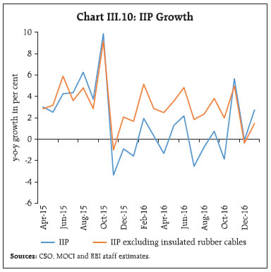 The impact of demonetisation on the manufacturing sector was transient - after contracting in December 2016, manufacturing output bounced back in January 2017. The manufacturing PMI, which had slipped in the contractionary zone in December 2016, expanded in January-March 2017. The performance of listed private companies remained resilient as sales and net profit growth improved at the aggregate level, although the performance of non-information technology (non- IT) service sector companies continued to be lacklustre (Chart III.11). Sales in cash intensive sectors such as fast moving consumer goods (FMCG) and motor vehicles declined in Q3 vis-à-vis the previous quarter (Chart III.12a and b). However, lead indicators such as passenger car sales and consumer durables suggest that this impact was short-lived. The electricity sector recorded a sharp increase in H2:2016-17 on a y-o-y basis. Although thermal electricity production remained weak, nonconventional sources such as solar and wind energy have registered higher production while pulling down the price. With India taking significant strides in expanding non-conventional sources of energy, helped by an enabling policy environment, and with the expected improvement in the financial health of power distribution companies (DISCOMs) after implementation of the Ujwal DISCOM Assurance Yojana (UDAY) scheme, the outlook for electricity generation has brightened considerably. III.2.4 Services The slowdown in the services sector, which became evident from Q1:2016-17, was sharper in H2:2016- 17. Some services sectors were adversely impacted by demonetisation, albeit temporarily, especially construction and realty. The implicit CSO data for Q4, however, suggests that these effects to be waning. Steel consumption and cement production - lead indicators of construction activity - remained positive from Q2:2016-17, although there was a sharp decline in cement production since December (Chart III.13). 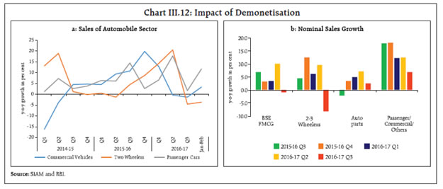
 The government’s continuing thrust on building infrastructure - as evident from a significant increase in both road projects awarded and constructed - and rural housing, should revive the construction sector in the period ahead. Trade, hotels, transport and communication are the other sectors, which are shrugging off the effects of demonetisation and gearing up for a revival. Tourist arrivals have picked up strongly in recent months. In the transport segment, major lead indicators such as commercial and passenger vehicles sales have revived from the lows of November/December 2016. Financial, real estate and business services have faced subdued conditions for the past four quarters as constraints on account of slowing bank credit pulled down its growth. Credit growth has continued to remain tepid, although insurance premiums witnessed a surge. The real estate segment, which largely reflects value addition by listed real estate companies, was impacted by demonetisation as evident in a sharp fall in the BSE realty index. Subsequently, these losses have been recouped as these transitory effects wore off. The business services segment largely reflects the performance of IT companies. Sales and profit of these companies remained robust. Nonetheless, the outlook for this segment is clouded by uncertainty in view of growing protectionist and anti-globalisation sentiments in the US. As alluded to earlier, public administration and defence continued to exhibit robust growth throughout 2016-17 due to higher expenditure on account of the 7th CPC award and OROP. Given the commitment to fiscal consolidation, however, double digit growth in these segments may not sustain in 2017-18. Overall, for the services sector, lead/coincident indicators suggest some recovery in Q4 from a prolonged downturn and the more immediate hit from demonetisation. III.3 Output Gap The efficacy of monetary policy critically depends on an accurate assessment of resource utilisation. In this context, a good fix on potential output is vital but challenging since it is unobservable. Estimation of potential output has to deal with uncertainty as real time measures of aggregate activity contain a considerable amount of noise and are often subject to significant revisions. The introduction of a new base year for national accounts (2011-12) and the continuing unavailability of a time series for previous years for ensuring appropriate degrees of freedom in econometric estimation are major impediments in this endeavour. Demonetisation added some uncertainty to the growth outlook, but its impact was transitory. For a fair assessment of the output gap for India, which indicates deviation of actual output from its potential level and expressed as percentage of potential output, the revised GVA data were augmented with forecasts applying different univariate filters such as the Hodrick-Prescott filter, the Baxter-King filter, the Christiano-Fitzgerald filter and a Multivariate Kalman (MKV) filter4. A MKV filter is particularly useful as it juxtaposes demand conditions with movements in inflationary pressures. The estimated output gap measures were aggregated by using principal components to get a composite measure, which indicates that the output gap (actual minus potential), is gradually closing (Chart III.14). Growth prospects are expected to strengthen in 2017-18 on account of several factors. First, discretionary consumer demand held down by demonetisation is expected to bounce back. Second, economic activity in cash-intensive sectors such as retail trade, hotels and restaurants, transportation as well as in the unorganised sector is getting rapidly restored. Third, demonetisation-induced ease in bank funding conditions has led to a sharp improvement in transmission of past policy rate reductions into marginal cost-based lending rates, and in turn, to lending rates for healthy borrowers, which should spur a pick-up in both consumption and investment demand. Fourth, the emphasis in the Union Budget for 2017-18 on the rural economy and affordable housing should also be positive for growth.
IV. Financial Markets and Liquidity Conditions Domestic market segments were shaped by local factors in an environment of heightened volatility in global financial markets. Large surplus liquidity in the money market post-demonetisation was managed with a mix of conventional and unconventional instruments. Volatility in the foreign exchange market remained contained, notwithstanding portfolio outflows. Credit growth, particularly to industry, remained depressed on asset quality concerns and weak investment demand. Equity and debt markets exhibited episodic price movements before stabilising by the end of the year. Since the October 2016 Monetary Policy Report (MPR), the appetite for risk in global financial markets has been punctuated by bouts of volatility triggered by the largely unanticipated US presidential election results in November, apprehensions of intensified protectionist measures by the US, and monetary policy tightening with unexpected hawkish guidance by the Fed in December. Thereafter, markets responded positively to the expectations of a significant reset of the policy mix in the US by the new administration sharpening focus on the fiscal policy. The strengthening of the US dollar, hardening of bond yields, a surge in equity markets on easing global deflation risks and a stronger growth outlook for advanced economies (AEs) triggered capital outflows from emerging market economies (EMEs). Consequently, fixed income markets and exchange rates in EMEs came under pressure. Volatility in markets of most EMEs, however, remained contained, unlike during the taper tantrum. More recently, EMEs have witnessed a resumption of portfolio flows. Domestic financial markets were impacted by twin shocks – demonetisation and the US presidential election results. The Union Budget announcements, the shift in the monetary policy stance of the Reserve Bank and new data releases relating to inflation and economic activity also influenced market movements. Demonetisation drove a wall of liquidity into the money market. War-time liquidity management by the Reserve Bank, however, limited the extent of softening of money market rates relative to the policy repo rate within the liquidity adjustment facility (LAF) corridor. G-sec yields moved in either direction, driven by different factors. While the announcement of a policy rate cut in October and demonetisation imparted a softening bias, tightening of monetary policy in the US, application of the incremental cash reserve ratio (ICRR) to absorb surplus liquidity, the status quo on monetary policy by the Reserve Bank in December and the shift in the monetary policy stance in February 2017 to neutral hardened yields. The rupee displayed two-way movements up to mid-January, but since then, it has appreciated on resumption of portfolio inflows in both the debt and equity segments. Surplus liquidity conditions impelled and lubricated the transmission of monetary impulses to deposit and lending rates. However, credit growth, particularly to industry, remained sluggish on risk aversion by banks due to high levels of stressed assets and weak demand in view of the depressed investment cycle and the presence of spare capacity in manufacturing. IV.1 Financial Markets IV.1.1 Money Market: In Q3 of 2016-17, the October policy repo rate cut was transmitted fully in the money market, amidst easy liquidity conditions. The unprecedented surge of liquidity after the announcement of demonetisation (details set out in Section IV.3) shocked the market. The efficacy of liquidity absorption operations by the Reserve Bank can be gauged from the fact that the weighted average call money rate (WACR) – the operating target of monetary policy – traded at only about 14 bps below the repo rate between November 9, 2016 and end- December 2016; it coursed 6 bps below during October 2016 to November 8, 2016. In Q4, the stepped-up pace of remonetisation resulted in some reduction in the liquidity surplus, which was still massive relative to the historical experience. A calibrated change in the mix of instruments for liquidity absorption from open market operations (OMOs) under the market stabilisation scheme (MSS) to reverse repo operations under the Reserve Bank’s LAF imparted a further softening bias to the WACR, which traded at 25 bps below the repo rate, on average. The usual year-end liquidity pressure stemming from banks’ balance sheet adjustments and tax payments to the Government did not spike money market rates, as the post-demonetisation liquidity overhang remained substantial. Other overnight money market rates, viz., collateralised borrowing and lending obligation (CBLO) and market repo, also traded in sync with the WACR, albeit with a downside bias of about 35 bps (Chart IV.1). 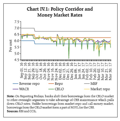 Country practices on the width of the policy corridor point to a considerable diversity, suggesting that the choice of the width of the corridor is time- and countryspecific (Table IV 1). In the Indian context, the recent overhang of large surplus liquidity – despite full absorption through the use of both conventional and unconventional instruments – has imparted a persistent downside bias to money market rates relative to the policy repo rate, which has spilled over to even 3-month money market rates, as discussed subsequently. The 3-month treasury bill (T-bill) rate has often stayed closer to the fixed reverse repo rate – or the floor of the LAF corridor – rather than the policy repo rate. Narrowing of the LAF corridor under such conditions can help in finer alignment of the operating target to the repo rate. This, in turn, could make overall money market conditions more consistent with the monetary policy stance. | Table IV.1: Monetary Policy Interest Rate Corridors of Select Countries | | Country | Monetary Policy Corridor Width (bps) | Country | Monetary Policy Corridor Width (bps) | | Australia | 50 (+/- 25) | Malaysia | 50 (+/- 25) | | Canada | 50 (+/- 25) | New Zealand | 50 (+50/0) | | Euro System | 65 (+25/-40) | Philippines | 100 (+/- 50) | | India | 100 (+/- 50) | Sweden | 150 (+/- 75) | | Indonesia | 150 (+/- 75) | Thailand | 100 (+/- 50) | | Japan | 40 (+30/-10) | United Kingdom | 50 (+50/0) | | Korea | 200 (+/- 100) | United States | 50 (+50/0) | | Sources: Central Bank websites of respective countries. | Demonetisation-induced surplus liquidity conditions also impacted the market micro structure, which had a bearing on volumes and rates. In the call money market, lending volumes of co-operative banks increased significantly. Their share in average daily call volumes rose to more than 50 per cent postdemonetisation (up to February 2017), from the average of 36 per cent during April-October 2016. These reported trades, as opposed to the transaction-based Negotiated Dealing System-Call (NDS-CALL) rates, pulled down the overall WACR, especially during later hours of the trading days. In the collateralised segments, mutual funds increased their lending in both the CBLO and market repo segments, enabled by large mobilisation of short-term funds, and consequently, collateralised rates traded below the WACR. Banks were active on the borrowing side in both the CBLO and market repo segments (accounting for about 74 per cent and 79 per cent of total daily average volumes, respectively, in February 2017), taking advantage of their lower cost of funds. Although many banks arbitraged between the various segments of the money market and the Reserve Bank’s LAF window, persistently high structural surplus liquidity heavily weighed on money market rates. Nonetheless, volatility in the WACR estimated from an IGARCH1 (1,1) model has been muted (Chart IV.2). In view of surplus liquidity, banks reduced recourse to certificates of deposit (CDs), issuance of which declined sharply to ₹407 billion and ₹850 billon during Q3 and Q4 (up to March 17, 2017) of 2016-17 as against ₹1,446 billion and ₹2,607 billion, respectively, during Q3 and Q4 of previous year (Chart IV.3). Liquidity also imparted a softening bias to the weighted average discount rates in primary issuance markets for commercial paper (CP). In the secondary markets, 3-month CD and 91-day T-bill rates softened by about 25 and 63 bps, respectively, while the 3-month CP rate declined by 30 bps. 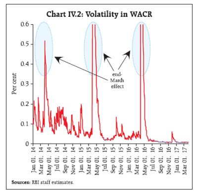 IV.1.2 Government Securities Market: Yields in the government securities (G-sec) market remained volatile in H2, induced by three major events (Chart IV.4). First, G-sec yields softened in October 2016 following the 25 bps policy repo rate cut by the Reserve Bank and the yield curve shifted downwards. Later during the month, however, yields moved up marginally tracking rising global yields on expectations of a Fed rate hike in December 2016. 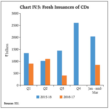
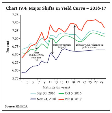 Second, G-sec yields softened significantly after the announcement of demonetisation and the resultant surge of liquidity in the system (Chart IV.5). The yield on the benchmark 10-year paper dropped from 6.80 per cent on November 8, 2016 to 6.19 per cent on November 24, 2016 (touching an intra-day low of 6.11 per cent on November 25, 2016, i.e., below the policy repo rate). Yields aligned with the policy rate in the first week of December 2016. Trading volumes in the secondary market reached an all-time high of ₹2,051 billion on November 21, 2016. In the primary market, 91-day T-bill yields plummeted to 5.86 per cent on November 23, 2016. 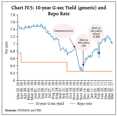 Yields hardened in December 2016 due to a number of factors: imposition of incremental CRR to absorb surplus liquidity in the banking system; portfolio outflows from the debt market following the hike in interest rate by the US Fed accompanied by the hawkish statement about future rate hikes; expectations of fiscal stimulus in the US (which pushed up US bond yields); rising crude oil prices; and the status quo on monetary policy announced by the Reserve Bank. Third, G-sec yields hardened in February 2017 and the yield curve steepened in response to the unexpected shift in the monetary policy stance of the Reserve Bank from accommodative to neutral, higher CPI inflation excluding food and fuel, and bunching of Ujwal DISCOM Assurance Yojana (UDAY) bonds with State Development Loans (SDLs) issuances, as discussed subsequently. The generic 10-year yield rose on the date of announcement of the change in the monetary policy stance in February by 31 bps to 6.93 per cent. The average daily closing of generic 10-year yield increased from 6.96 per cent in February 2017 to 7.13 per cent in March 2017. Higher domestic yields since February, inter alia, have contributed to the return of portfolio flows to the debt market (Chart IV.6). From October 2016 to January 2017, there were net FPI outflows of around ₹336 billion from the Indian G-sec market. Since February, however, there have been net FPI inflows of about ₹229 billion. Fiscal developments had a bearing on G-sec yields during Q4. The Central Government reduced its market borrowings in Q4 of 2016-17 by ₹180 billion through dated securities and ₹510 billion through T-bills, which reduced the supply of sovereign paper in the market. The Government announced net market borrowings for 2017-18 in the Union Budget at ₹4,232 billion (BE), which included planned buyback of securities of ₹750 billion. The Union Budget has also provided for ₹250 billion for switching of securities, which is a debt management strategy that aims at reducing near-term redemption pressure and elongating the maturity of debt. State Governments’ reliance on market borrowings for funding their fiscal deficit has increased steadily in recent years. Large issuances of SDLs by States have been exerting upward pressure on yields (Chart IV.7). The spread of SDLs cut-off over the 10-year G-sec increased persistently in the second half of 2016-17 – from 28-49 bps in October 2016 to 86-114 bps in March 2017. As regards UDAY bonds, issuances during the previous year were at a fixed spread of 75 bps over the corresponding/10-year FIMMDA G-sec yields. The spreads for issuances of UDAY bonds during 2016-17, however, came down to the range of 35-75 bps, following the modification in the issuance strategy to invite bids from all the market participants. 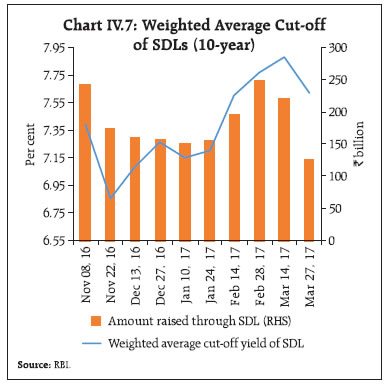 IV.1.3 Corporate Bond Market: The corporate bond yield (AAA 5-year benchmark) softened from 7.52 per cent in October 2016 to 7.33 per cent in January 2017, tracking the movements in G-sec yields on surplus liquidity conditions after demonetisation. However, after the February monetary policy announcement, the corporate bond yield hardened to 7.65 per cent before declining to 7.56 per cent at end-March 2017. Taking advantage of low yields and tight credit market conditions because of stressed assets in the banking system, corporates mobilised higher resources from the corporate bond market, i.e., ₹2,502 billion during October 2016 – February 2017 as against ₹1,957 billion during the corresponding period of the previous year (Chart IV.8). Private placements constituted 97.8 per cent of the total amount mobilised. Indian corporates also raised large resources by way of bonds from international markets (Chart IV.9). Foreign portfolio investment in the corporate bond market declined during November 2016 to January 2017 on account of risk-off strategies followed by international investors. Portfolio flows turned positive from February due to global risk-on portfolio shifts and also to take advantage of higher domestic yields. Several measures were announced to deepen the corporate bond market: (i) enhancing the aggregate limit of partial credit enhancement (PCE) provided by banks to 50 per cent; (ii) permitting brokers in corporate bond repos; and (iii) allowing consolidation and re-issuance of corporate bonds. The turnover in the corporate bond market (in terms of amount) increased by 63.8 per cent during H2, which was a record high. In US dollar terms, the turnover increased from US$ 6.0 billion in H2:2015-16 to US$ 9.7 billion in H2: 2016-17. IV.1.4 Stock Market: The stock market (BSE Sensex) gained by 6.3 per cent in H2:2016-17 (Chart IV.10). In October 2016, the stock market remained volatile due to factors such as increasing prospects of an interest rate hike by the US Fed in December and consequent portfolio outflows, and mixed corporate results for Q2. Following the 25 bps cut in the repo rate by the Reserve Bank in October 2016, it gained modestly. During November 2016, the BSE Sensex plunged by 4.6 per cent on uncertainty over the impact of demonetisation on economic growth and corporate earnings and also portfolio equity outflows triggered by the risk-off market reactions to the US presidential election results. Demonetisation had a relatively greater impact on cash sensitive sectors such as FMCG, consumer durables, auto and realty vis-a-vis the overall Sensex. The downward bias persisted during December on sustained selling by foreign institutional investors, subdued auto sales data for November, persisting concerns about Q3 earnings, and the interest rate increase by the US Fed but with unexpected hawkish guidance.  The stock market revived in January 2017 due to value buying by domestic institutional investors, better than expected quarterly corporate results for Q3, revival of foreign portfolio equity investment from mid-January and positive cues from global markets. The recovery continued in February 2017 on proposals made in the Union Budget, particularly a lower fiscal deficit target for 2017-18, exemption of category I and category II foreign portfolio investors from taxation on indirect transfers, and an unchanged capital gains tax rate for the capital market. FPIs stepped up buying following the status quo maintained by the US Fed and positive cues from global equity markets. The impact of demonetisation on sectoral indices was transitory as they have recovered their losses and scaled higher than their pre-demonetisation levels. In March, the stock market gained further on better than expected Q3 GDP growth estimates in India released by the CSO, PMI for both manufacturing and services for the month of February pointing to expansion after the demonetisation-induced contraction, and approval of the draft Central GST (CGST) and Integrated GST (IGST) bills by the GST Council.2 Despite the Fed rate increase in March, which was already priced in by markets, the dovish stance improved appetite for risk assets, including in EMEs. On expectations that the State election results would provide the impetus for reforms, the BSE Sensex (29,974) and Nifty (9,265) closed at all time highs on April 5, 2017. IV.1.5 Foreign Exchange Market: In the foreign exchange market, the rupee moved in a narrow range against the US dollar and appreciated against the euro and pound sterling in H2 of 2016-17 (Chart IV.11). In Q3, the weakness of the rupee against the US dollar mainly reflected the strengthening of the dollar following the US presidential election outcome; FPI outflows (both in equity and debt); increased demand from oil importers for foreign currency; FCNR(B) redemption pressures; and the policy rate cut in October 2016. The US dollar strengthened in anticipation of an expansionary fiscal policy and tighter monetary policy by the Fed. Consequently, the rupee depreciated against the US dollar by 2.9 per cent (from ₹66.71 per US dollar on November 8 to ₹68.72 on November 28). The rupee regained about half of the lost ground by the first week of December 2016, but came under renewed downward pressure till end-January 2017 in response to the Fed policy rate hike. From February 2017 onwards, the rupee has appreciated due to equity portfolio inflows on policy announcements made in the Union Budget and easing of concerns about the speed of Fed policy rate hikes. Factors such as India’s low current account deficit, the emphasis of monetary policy on the 4 per cent inflation target, the transient impact of demonetisation on economic activity, and the commitment to fiscal prudence announced in the Union Budget provided stability to the exchange rate. The rupee gained further in March as FPI inflows, especially equity, were boosted by the outcome of State elections, which augur well for accelerating the pace of reforms. 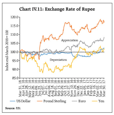
| Table IV.2: Nominal and Real Effective Exchange Rates: Trade-Based (Base: 2004-05=100) | | Item | Index: March 31, 2017 (P) | Appreciation (+) / Depreciation (-) (per cent) | | Mar 31, 2017 over Mar 31, 2016 | Mar 31, 2017 over Sep 30, 2016 | | 36-currency REER | 119.3 | 7.9 | 4.2 | | 36-currency NEER | 78.3 | 6.3 | 5.2 | | 6-currency REER | 132.2 | 7.8 | 5.0 | | 6-currency NEER | 70.8 | 6.3 | 6.1 | | ₹/ US$ (As on March 31, 2017) | 64.8 | 2.3 | 2.8 | P: Provisional.
Note: REER figures are based on Consumer Price Index (Combined).
Source: RBI. | In terms of both 36-currency nominal effective exchange rate (NEER) and real effective exchange rate (REER), the rupee appreciated by 6.3 per cent and 7.9 per cent, respectively, between end-March 2017 and end-March 2016 (Table IV.2). IV.1.6 Credit Market: In the credit market, y-o-y growth in non-food credit decelerated through H2 to a low of 4.7 per cent in early January before picking up to 5.1 per cent by March 17, 2017. Several factors, however, overstate this slowdown. As outlined in the October 2016 MPR, credit flows were impacted by loan write-offs and swapping of bank credit into special securities under the UDAY (Chart IV.12). In addition, the use of specified bank notes (SBNs) for repaying loans would have also dampened the growth rate of bank credit. From the demand side, a depressed investment cycle, persisting excess capacity in manufacturing, and deleveraging on the part of corporates to improve their credit ratings (as explained in Chapter III) have contributed to the slowdown in credit growth. The deceleration in credit growth also highlights the role of supply side factors – stressed assets and capital constraint – in hindering a revival in the credit cycle (Box IV.1 and Chart IV.13). Box IV.1: Stressed Assets, Capital Constraints and Supply of Credit The “capital crunch hypothesis”, i.e., capital constrained banks cutting back on lending, was highlighted as a key factor that worsened the US recession in the early 1990s (Bernanke and Lown, 1991). Since then, theoretical and empirical literature has firmly established the role of a “capital channel” that operates from the supply side of credit, as opposed to the typical focus of monetary policy transmission on the demand side (Rivera, 2015). Two arguments are highlighted in the debate on the role of bank capital in conditioning the credit cycle. First is the endogenous money view, which indicates that banks can always fully meet the demand for loans from all credit-worthy borrowers, and no funding constraint (posed by the composition of liabilities in terms of equity versus debt) can prevent banks from doing so. This macro view is in sync with the Modigliani and Miller argument on the irrelevance of capital structure as applied to banks, i.e., the composition of liabilities of banks should not influence the price and quantity of credit. Second, the post-Keynesian emphasis on credit rationing under which borrowers, that cannot meet tighter credit standards set by banks (say, amidst a recession or heightened uncertainty that may change the risk assessment of banks), fail to access credit. Thus, not all demand for credit is met. When banks face a loss of confidence (arising, for example from unanticipated large increase in stressed assets), they need more capital to bolster their loss absorbing capacity. Raising capital from equity holders, however, becomes difficult, costlier and unattractive in such a situation, forcing banks to deleverage instead. This may also reflect the natural eventual outcome of the lack of market and regulatory discipline and the tendency to evergreen bad loans. An adverse feedback loop sets in, under which inadequate capital leads to cut backs on lending to viable projects. In turn, this deepens a recession, which increases stressed assets and reduces capital further. Using panel data for the Indian banking system (quarterly data of 66 banks for the period Q1 of 2009 to Q4 of 2016) and applying four different models (i.e., fixed effects, random effects, difference and system generalised method of moments (GMM) following Arellano-Bond/Bond-Bover) to check for the robustness of estimates, it is found that the gross non-performing assets (GNPA) and capital to risk weighted assets ratio (CRAR) significantly influence credit growth. While better capitalised banks exhibit higher credit growth, banks with higher GNPAs experience weaker credit growth (Table 1). | Table 1: Determinants of Bank Lending (Dependent variable: Δlcredit) | | | Random Effect Model | Fixed Effect Model | AB- Diff. GMM | AB-System GMM | | Δlcreditt-1 | -0.12*** | -0.15** | -0.18* | -0.15** | | | (-1.7) | (-2.2) | (-3.0) | (-2.1) | | gnpat | -0.64* | -0.64* | -0.56* | -0.63* | | | (-7.6) | (-5.1) | (-4.5) | (-7.5) | | crart | 0.16* | 0.25* | 0.36** | 0.16* | | | (5.9) | (5.3) | (3.3) | (6.0) | | No. of Observations | 1848 | 1848 | 1782 | 1848 | | ar1 (p-value) | | | 0.01 | 0.01 | | ar2 (p-value) | | | 0.20 | 0.30 | | Hansen (p-value) | | | 1.00 | 1.00 | Notes: Δlcredit: credit growth (q-o-q); gnpa: gross non-performing assets to advances ratio; crar: capital to risk weighted assets ratio.
Estimations are controlled for seasonality, nominal GVA growth, return on equity and repo rate adjustments.
Figures in parentheses are z-statistics;
ar1 and ar2 are tests for first-order and second-order serial correlation, respectively.
Hansen tests are for checking the over-identifying restrictions for the GMM estimators.
*,**,***: Significant at 1%, 5% and 10% levels, respectively. |
Low net interest margin (NIM) is an indicator of efficient intermediation. However, when faced with large stressed assets, banks may either (i) strive to maintain/increase their NIMs and/or (ii) reduce supply of credit. Panel data (quarterly data of 72 banks for the period Q2 of 2010 to Q4 of 2016) regression results suggest that credit risk proxied by the stressed assets (i.e., restructured assets plus gross NPAs) to total assets ratio has a positive and statistically significant relationship with NIM of banks as a percentage of their total assets (Table 2). Regression results also indicate that one (positive) standard deviation shock to stressed assets could lead to about 0.15 standard deviation increase in NIM. | Table 2: Determinants of Net Interest Margin | | | AB – Difference GMM | AB – System GMM | | NIM(-1) | 0.542* | 0.568* | | Stressed Assets | 0.011* | 0.008* | | CRAR | 0.003* | 0.003* | | Bank Fixed Effects | No | Yes | | No of observations | 1944 | 1944 | Notes: NIM = (Interest income minus interest expense) to total assets (in per cent). Stressed assets = (Restructured assets plus gross NPAs) to total assets (in per cent).
The regressions are controlled for seasonality, credit growth, bank size, return on assets, operating expense, non -interest income, investment in SLR securities, GVA growth and inflation.
Hansen test for over identification restrictions and Arellano-Bond test for residual auto correlations are found to be satisfactory.
*:Significant at 1% level. | It is observed that banks could protect their NIM up to Q3:2014-15. Thereafter, however, their NIM declined, which also coincided with the sustained deceleration in credit growth. After the Asset Quality Review initiated in April 2015, decline in income associated with the explicit recognition of NPAs lowered the NIM. This amplified risk aversion and led to further deceleration of credit growth. References: Bernanke, Ben S and Cara S Lown (1991), “The Credit Crunch”, Brooking Papers on Economic Activity, 2. Rivera, Alvaro Santos (2015), “Bank Capital and Endogenous Money: Liquidity Preference and Capital Constraints as Determinants of Credit Rationing”, ECB, October. Sectoral data on flow of credit indicate that deceleration in credit, though broad-based, was characterised by a sharp contraction in exposure to industry (Chart IV.14). There was decline in credit in 12 of the 18 major industry sub-groups on a y-o-y basis as of February 2017. While the availability of funding from banks remained weak, the flow of credit from NBFCs3 during the first three quarters of 2016-17 was about 50 per cent higher than in the whole of 2015-16 (Chart IV.15). 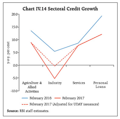 However, the overall flow of financial resources to the commercial sector in 2016-17 (up to mid-March) was lower than in the corresponding period of the previous year due to lower lending from banks. Among non-bank sources, funding from foreign sources increased due to marginally higher FDI inflows and a sharp increase in short-term credit. Financing through domestic sources increased primarily due to higher funding from NBFCs, subscription to commercial paper by non-banks and private placement by non-financial entities, notwithstanding diminished public issues (Table IV.3). IV.2 Monetary Policy Transmission Monetary policy transmission strengthened in H2 of 2016-17, aided by the surfeit of liquidity. The share of low cost current account and savings account (CASA) deposits in aggregate deposits with the SCBs went up to 39.2 per cent (as on March 17, 2017) – an increase of 4.0 percentage points relative to the predemonetisation period. Given the prevailing risk aversion, banks reduced their term deposit rates. The median term deposit rate and the weighted average domestic term deposit rate (WADTDR) fell by 37 bps and 32 bps, respectively, during November 2016-March 2017.4 Combined with the sharp increase in CASA deposits, the overall cost of borrowings declined, creating space for banks to cut their marginal cost of funds based lending rates (MCLRs). The one-year median MCLR declined by a cumulative 70 bps since November 2016, even as the policy rate remained unchanged. This is significant, given that the decline during the preceding seven months (April-October 2016) – when the repo rate was cut by 50 bps – was only 15 bps (Chart IV.16). Post-demonetisation (up to March 2017), 27 public sector banks have reduced their one-year median MCLR in the range of 50 to 105 bps, and 19 private sector banks have done so in the range of 25 to 148 bps. 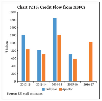
| Table IV.3: Flow of Financial Resources to the Commercial Sector | | (₹ billion) | | Item | April 1 to March 17 | | 2015-16 | 2016-17 | | ₹ billion | % of Total | ₹ billion | % of Total | | A. Adjusted Non-food Bank Credit (NFC) | 7,754 | 54.8 | 4,818 | 38.2 | | i) Non-Food Credit | 7,024 | 49.6 | 3,655 | 29.0 | | ii) Non-SLR Investment by SCBs | 731 | 5.2 | 1,164 | 9.2 | | B. Flow from Non-banks (B1+B2) | 6,403 | 45.2 | 7,802 | 61.8 | | B1. Domestic Sources | 4,479 | 31.6 | 5,511 | 43.7 | | 1 Public issues by non-financial entities @ | 363 | 2.6 | 120 | 1.0 | | 2 Gross private placements by non-financial entities @ | 985 | 7.0 | 1,599 | 12.7 | | 3 Net issuance of CPs subscribed to by non-banks | 1,173 | 8.3 | 1,467 | 11.6 | | 4 Net Credit by housing finance companies # | 706 | 5.0 | 849 | 6.7 | | 5 Total accommodation by the 4 RBI regulated All India Financial Institutions @ | 459 | 3.2 | 218 | 1.7 | | 6 NBFCs-D and NBFCs-ND-SI (net of borrowings from banks/FIs/CPs) # | 583 | 4.1 | 1,027 | 8.1 | | 7 LIC's net investment in corporate debt, infrastructure and social sector * | 210 | 1.5 | 230 | 1.8 | | B2. Foreign Sources | 1,924 | 13.6 | 2,290 | 18.1 | | 1 External Commercial Borrowings / FCCB @ | -329 | -2.3 | -412 | -3.3 | | 2 ADR/GDR Issues excluding banks and financial institutions @ | 0 | 0.0 | 0 | 0.0 | | 3 Short-term credit from abroad # | -274 | -1.9 | 167 | 1.3 | | 4 Foreign Direct Investment to India * | 2,527 | 17.8 | 2,535 | 20.1 | | C. Total Flow of Resources (A+B) | 14,157 | 100.0 | 12,620 | 100.0 | Note: Data are provisional. #: Up to December. *:Up to January. @: Up to February.
Sources: RBI, LIC, NABARD and SEBI. | 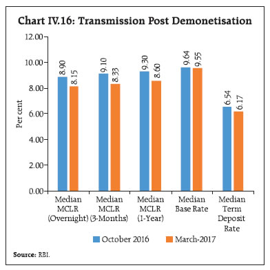 In comparison with deposit rates and the MCLR, transmission to actual lending rates has been less complete during the post-demonetisation period. During November 2016 – February 2017, the weighted average lending rate (WALR) of banks in respect of fresh rupee loans declined by 69 bps, whereas the WALR on outstanding rupee loans declined by 13 bps only over the same period. Transmission to lending rates for outstanding rupee loans vis-à-vis fresh rupee loans has been limited essentially on account of two factors. First, a major portion of loans contracted prior to the introduction of MCLR (i.e., April, 2016) has continued to be priced at the base rate5; in fact, loans contracted at the base rate still constitute about 67 per cent of banks’ loan portfolios. Second, even under the MCLRbased pricing of credit, the interest rate is typically reset on the existing loans on an annual basis, implying that most loans under the MCLR regime contracted up to December 2016 would not have benefited from the sharp reduction in the MCLR. An analysis of factors hindering transmission using quarterly bank level data (for the first three quarters of 2016-17) suggested the presence of a positive correlation between the spread (i.e., WALR on outstanding/fresh rupee loans over MCLR) and stressed assets of banks, implying that banks charge additional risk premiums on their performing assets to compensate for the interest income losses from NPAs. Among the various components of the MCLR, it is only the term deposit rates that are seen to respond to the changes in policy rate. Another factor which has impeded monetary policy transmission is the interest rates on small savings which are not in alignment with movements in market interest rates. Although the government has announced to revise the interest rates on small savings in line with the change in G-sec yields, this is not fully implemented (Box IV.2). IV.3 Liquidity Conditions and the Operating Procedure of Monetary Policy The amended RBI Act 1934 requires the Reserve Bank to place the operating procedure relating to the implementation of monetary policy and changes thereto from time to time, if any, in the public domain. This operating procedure – embodied in the Reserve Bank’s liquidity management framework – was published in Box IV.I of the April 2015 MPR. The operating procedure is guided by the objective of aligning the operating target of monetary policy – the weighted average call money rate (WACR) – to the repo rate through active liquidity management, consistent with the stance of monetary policy. The framework was modified in April 2016, details of which were presented in the October 2016 MPR. Consistent with the assurance given on proactive management of both permanent and frictional liquidity under the modified liquidity management framework of April 2016, and the guidance of moving the system from an average deficit equivalent to one per cent of net demand and time liabilities (NDTL) to a position of neutrality, the Reserve Bank injected permanent liquidity to the tune of ₹1.9 trillion during April-October 2016, primarily through open market purchase auctions of ₹1.1 trillion. The balance reflected the liquidity impact of forex market operations of the Reserve Bank and repurchase of securities by the Government. Box IV.2: Transmission to Small Savings Rates Although G-sec yields (10-year maturity) declined through 2016-17 (by about 79 bps), small savings rates remained unchanged for Q2 and Q4:2016-17, and were reduced only by 10 bps each for Q3:2016- 17 and Q1:2017-18. At the time of the introduction of the formula based reset of rates linked to G-sec yields for Q1:2016-17, interest rates on small savings were broadly aligned to the interest rates derived from the formula for fixing the interest rate on small savings. This spread between the actual rate of interest and the formula based interest rate increased to a range of 61 to 95 bps in Q1:2017-18 for different savings instruments (Table). The wide spread between small savings rates and bond yields makes small savings more attractive vis-à-vis bank deposits and discourages banks to fully adjust their deposit interest rates on fear of losing deposits, thereby hampering monetary transmission. | Table: Interest Rates on Small Savings Instruments for Q1: 2017-18 | | Small Savings Scheme | Maturity (years) | Spread
(Percentage point)** | Average G-sec yield (Per cent) of corresponding maturity
(Dec 2016 to Feb 2017) * | Formula** based rate of interest (Per cent) (applicable to Apr- Jun 2017) | GoI announced rate of interest (Per cent) (applicable to Apr-Jun 2017) | Difference (Percentage point) | | (1) | (2) | (3) | (4) | (5) = (3) + (4) | (6) | (7) = (6) - (5) | | Savings Deposits | - | - | - | - | 4.0 | - | | Public Provident Fund | 15 | 0.25 | 6.99 | 7.24 | 7.9 | 0.66 | | Term Deposits | | | | | | | | 1 Year | 1 | 0 | 6.09 | 6.09 | 6.9 | 0.81 | | 2 Year | 2 | 0 | 6.20 | 6.20 | 7.0 | 0.80 | | 3 Year | 3 | 0 | 6.31 | 6.31 | 7.2 | 0.89 | | 5 Year | 5 | 0.25 | 6.54 | 6.79 | 7.7 | 0.91 | | Post Office Recurring Deposit Account | 5 | 0 | 6.31 | 6.31 | 7.2 | 0.89 | | Post Office Monthly Income Scheme | 5 | 0.25 | 6.50 | 6.75 | 7.6 | 0.85 | | Kisan Vikas Patra | 113 Months | 0 | 6.99 | 6.99 | 7.6 | 0.61 | | NSC VIII issue | 5 | 0.25 | 6.70 | 6.95 | 7.9 | 0.95 | | Senior Citizens Saving Scheme | 5 | 1.00 | 6.54 | 7.54 | 8.4 | 0.86 | | Sukanya Samriddhi Account Scheme | 21 | 0.75 | 6.99 | 7.74 | 8.4 | 0.66 | *: Compounding frequency varies across instruments.
** : As announced by the Government of India on February 16, 2016.
Source: Government of India. | Following the announcement of demonetisation on November 8, 2016 and the subsequent surge in bank deposits, the Reserve Bank expanded the range of instruments for absorbing a record level of surplus liquidity. At the beginning of Q3, injection of permanent liquidity consistent with the assurance given under the modifications to liquidity management framework in April 2016, had already moved the system to an average surplus of ₹293 billion in Q2. As cash balances of the government increased and festival related currency demand drained liquidity out of the banking system, the average system wide surplus declined to ₹63 billion in October. After demonetisation, currency in circulation declined by ₹8,997 billion (up to January 6, 2017). This sudden increase in liquidity in the banking system, coupled with the weak demand for credit (as explained in Section IV.1), necessitated a significant step up in the liquidity absorption operations by the Reserve Bank so that money market rates remained consistent with the policy repo rate. The Reserve Bank used a mix of both conventional and unconventional instruments, viz., (i) temporary application of an ICRR of 100 per cent on the increase in NDTL of banks between September 16 and November 11, 2016; (ii) open market sales of cash management bills (CMBs) issued under the MSS to manage the large surplus liquidity; and (iii) variable rate reverse repos of various tenors (Chart IV.17). The peak level of liquidity absorbed reached ₹7,956 billion on January 4, 2017 (₹2,568 billion absorbed through reverse repos and ₹5,466 billion through CMBs under the MSS). 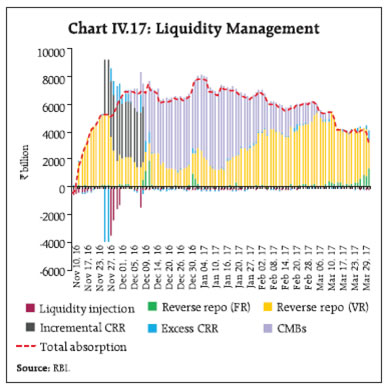 The ICRR was in place for one fortnight (ended on December 9, 2016). It helped in draining excess liquidity from the system to the extent of about ₹4,000 billion. With the enhancement of the limit on issuance of securities under the MSS from ₹300 billion to ₹6,000 billion on December 2, 2016 by the Central Government, the Reserve Bank withdrew the ICRR. Thereafter, it managed surplus liquidity conditions through the use of fine tuning reverse repos and the MSS. In Q4, remonetisation progressed at an accelerated pace, with currency in circulation increasing cumulatively by about ₹4,373 billion (Chart IV.18). This reduced the liquidity surplus in the system to ₹3,141 billion by end-March 2017. 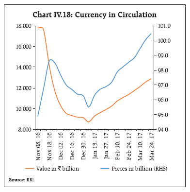
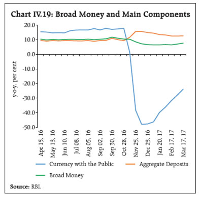 In anticipation of the liquidity surplus declining further due to remonetisation, the Reserve Bank increasingly resorted to reverse repo operations to absorb the surplus liquidity released by maturing CMBs, especially from January 14, 2017. The Reserve Bank absorbed daily average surplus liquidity of ₹4,024 billion in Q3 (after demonetisation) and ₹5,932 billion in Q4. This ensured the alignment of the WACR with the policy repo rate, albeit with a soft bias. Post-demonetisation, currency in circulation contracted as SBNs were returned by the public and correspondingly, deposits with banks increased sharply (Chart IV.19). Although a sharp moderation in the currency deposit ratio led to an increase in the money multiplier, it could not offset the impact of the contraction in base money (by about 22 per cent as on March 17, 2017 from the period immediately prior to demonetisation) on broad money (M3). Structural surplus liquidity enabled banks to meet the liquidity coverage ratio (LCR) requirement, which was tightened from 70 per cent to 80 per cent in January 2017. The excess statutory liquidity ratio (SLR) position of banks was about 11 per cent on an average in Q4 of 2016-17 (up to February), which included investment in CMBs under the MSS and excess liquidity parked with the Reserve Bank under reverse repo operations (Chart IV.20). 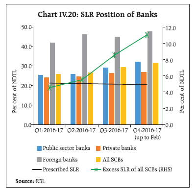 Looking ahead, liquidity conditions are expected to remain in surplus in the short-run, which the Reserve Bank would continue to modulate so that money market rates remain consistent with the operating target and the stance of monetary policy. Progressively greater use of term reverse repos to absorb the surplus liquidity should contribute to the development of the term money market. The change in the monetary policy stance from accommodative to neutral in February 2017 has altered market expectations, but the transmission of past cumulative 175 bps cut in the repo rate to lending rates remains incomplete. Resolution of stressed assets and recapitalisation of public sector banks will be critical to ease risk aversion by banks. This will enhance the flow of credit to productive sectors and also improve monetary policy transmission.
V. External Environment Global economic activity and trade picked up modestly from the later part of 2016. The firming up of commodity prices led to some uptick in inflation in major advanced economies (AEs). Recessionary conditions ebbed in key commodity exporting emerging market economies (EMEs), setting the stage for a turnaround in EMEs as a group. Since the MPR of October 2016, global growth picked up modestly towards end-2016, and is projected to improve further in 2017 by multilateral agencies. Growth in EMEs moderated in 2016, but is set to improve with the ebbing of recessionary conditions in key commodity exporting countries. Even though world trade appeared to have emerged out of a trough, new risks have emerged from an increasing tendency towards protectionist policies and heightened political tensions. Commodity prices have risen since late 2016 on improvement in US economic indicators such as strong labour market and consumer spending; infrastructure spending in China; and geopolitical concerns. Crude oil prices firmed after the OPEC announced curtailment of production. Inflation edged up on expectations of reflationary fiscal policies in the US, rising energy prices and a mild strengthening of demand. International financial markets were impacted by the US election results and expectations of monetary policy tightening by the Federal Reserve, underpinned by hawkish forward guidance. Financial markets in EMEs briefly turned volatile after the US election due to large capital outflows leading to plunges in currency and equity markets. Nevertheless, average volatility remained contained by historical standards since Q4:2016. Bond yields hardened across the globe in tandem with US yields, before softening somewhat since mid-March. Strengthening of the US economy further buoyed the equity markets, while the increasing likelihood of more rate hikes by the Federal Reserve in 2017 hardened bond yields in AEs. The US dollar appreciated to a multi-year high in December and remained bullish. V.1 Global Economic Conditions The US economy bounced back strongly in Q3:2016, underpinned by robust consumer spending and continuing improvement in the labour market. GDP growth decelerated sharply in Q4:2016 due to a large slippage in net exports, even though retail sales, consumer confidence and the purchasing manufacturers’ index (PMI) suggested sustained momentum. Domestic demand grew (q-o-q) at the fastest pace in almost two years. Consumer confidence reached a 16-year high in March, though retail sales had slowed down in February. The Institute for Supply Management’s (ISM) index suggested manufacturing expanded at its fastest pace in three years in February. In the Euro area, GDP growth accelerated in H2:2016. Relatively low oil prices and sustained employment gains have provided support to household incomes. Improving consumer confidence and the PMI, which rose to a six-year high in March, indicate that activity continued to expand in Q1:2017. Nonetheless, the region remains vulnerable to a number of headwinds such as the formal beginning of the Brexit process, upcoming elections in several constituent countries and tightening of financial conditions. The Japanese economy continued to recover at a modest pace even as the momentum weakened in H2:2016. Increases in private consumption and fixed investment were moderate, although there was some uptick in exports and industrial production towards end-2016. The manufacturing PMI improved during January and February but moderated again in March 2017. In the UK, economic growth gained momentum in H2: 2016, notwithstanding the uncertainties surrounding the negotiations relating to Brexit, as exports rose substantially following the weakening of the pound. However, manufacturing growth weakened for two consecutive months in February, indicating the possibility of a slowdown in 2017 (Table V.1). Economic activity in EMEs continued to be divergent. In China, even though y-o-y GDP growth improved in Q4:2016, supported by policy stimulus and the rising property market, q-o-q growth showed a sharp loss of momentum. Industrial production and PMI stabilised, but there are rising concerns about high indebtedness and financial stability. Consequently, the growth target for 2017 has been reduced to about 6.5 per cent by the government. In Brazil, the economic situation seems to have improved with the rise in commodity prices and several measures such as reforming the bankruptcy law announced by the authorities to revive growth. Economic contraction has eased in Russia, with the improvement in the mining and manufacturing sectors, rise in oil prices and policy initiatives that included a more flexible exchange rate and bank recapitalisation. In South Korea, Thailand and Mexico, GDP growth lost some momentum in Q3 and Q4:2016. According to the IMF, growth in both AEs and EMEs will pick up in 2017. The OECD’s composite leading indicators (CLIs) point to growth accelerating in the US, Japan, China, Brazil and Russia, stable momentum in the Euro area and tentative signs of emerging momentum in the UK. However, manufacturing activity remains weak in some countries as underscored by the PMIs (Chart V.1). | Table V.1: Real GDP Growth (q-o-q, saar) | | (Per cent) | | Country | Q4-2015 | Q1-2016 | Q2-2016 | Q3-2016 | Q4-2016 | 2017 (P) | 2018 (P) | | Advanced Economies (AEs) | | US | 0.9 | 0.8 | 1.4 | 3.5 | 2.1 | 2.3 | 2.5 | | Euro area | 2.0 | 2.0 | 1.2 | 1.6 | 1.6 | 1.6 | 1.6 | | Japan | -1.0 | 1.9 | 2.2 | 1.2 | 1.2 | 0.8 | 0.5 | | UK | 2.8 | 0.8 | 2.4 | 2.0 | 2.8 | 1.5 | 1.4 | | Canada | 0.5 | 2.7 | -1.2 | 3.8 | 2.6 | 1.9 | 2.0 | | Korea | 2.8 | 2.0 | 3.6 | 2.0 | 2.0 | 3.0 | 3.1 | | Emerging Market Economies (EMEs) | | China | 6.0 | 5.2 | 7.6 | 7.2 | 6.8 | 6.5 | 6.0 | | Brazil | -4.8 | -2.4 | -1.3 | -2.9 | -3.6 | 0.2 | 1.5 | | Russia* | -3.2 | -0.4 | -0.5 | -0.4 | 0.3 | 1.1 | 1.2 | | South Africa | 0.5 | -1.5 | 3.1 | 0.4 | -0.3 | 0.8 | 1.6 | | Thailand | 2.5 | 4.3 | 4.2 | 1.7 | 1.7 | 3.3 | 3.1 | | Malaysia | 4.8 | 4.0 | 2.8 | 5.6 | 5.6 | 4.6 | 4.7 | | Mexico | 1.6 | 1.9 | 0.4 | 4.2 | 2.8 | 1.7 | 2.0 | | Saudi Arabia* | 4.3 | 2.0 | 1.5 | 0.9 | 1.2 | 0.4 | 2.3 | | Memo: | | | 2016 (E) | 2017 (P) | 2018 (P) | | World Output | 3.1 | 3.4 | 3.6 | | World Trade Volume | 1.9 | 3.8 | 4.1 | E : Estimate, P : Projection, *: y-o-y growth.
Sources: Bloomberg and IMF. | World trade growth improved in Q4:2016, largely supported by EMEs as imports by AEs moderated. In January 2017, exports rebounded sharply in China and Brazil. Exports also increased in some East Asian economies. Merchandise and services trade improved (in nominal terms), although it remained below its long-term average (Chart V.2). The IMF and the World Bank project higher growth in world trade volumes in 2017. The World Trade Outlook Indicator of the World Trade Organisation (WTO) and the global PMI for new export orders also indicate strengthening of world trade growth momentum in Q1:2017. There are, however, several downside risks emanating from heightened policy uncertainty in the US and the UK from proposals to retreat from multilateral/regional trade agreements, raising of tariffs and non-tariff barriers and consequent retaliation. Furthermore, the medium-term trade outlook is expected to remain weak and is unlikely to revert to its pre-crisis level as several structural factors have led to a decline in the income elasticity of world trade. The recovery in world trade could, however, diverge significantly across various regional blocs (Box V.1). Box V.1: Global Economic Activity and Trade: A New Normal? Since the second half of 2011, global trade growth has remained slower than the expansion in world GDP, while in the 25 years before the global financial crisis, trade growth was twice the GDP growth. Thus, the income elasticity of trade has fallen sharply in the post-crisis years. Two main developments with roughly equivalent contributions, viz., compositional effects and structural factors, have been the driving forces in the slowdown in trade vis-à-vis economic growth. Compositional effects include shift in economic activity and trade from AEs towards EMEs, the declining share of the import-intensive component of global demand and shift in trade from manufacturing to services. These factors may not necessarily be structural and could revert in the medium-term when the global economy recovers fully. Structural factors, which set in well before the global recession, reflect fundamental shifts working through at least three channels. First, lower transportation costs, removal of trade barriers and increase in multilateral global trade agreements, which contributed to expansion in global trade, have waned. Second, global value chains (GVCs) have slowed down sharply, partly due to rising labour costs in EMEs and partly on account of rising protectionism. Third, financial deepening which facilitated export activity has diminished. The interplay of these factors suggests that the relationship between growth and trade may be approaching a new normal (ECB, 2016). Following Constantinescu et al. (2015), an error correction model (ECM) on monthly data for the period January 2000 to July 2016 was specified as follows: Bai-Perron tests suggest at least three regimes in the model, viz., January 2000 to October 2008; November 2008 to April 2011; and May 2011 to July 2016, broadly coinciding with the pre-crisis period, the crisis period and the post-crisis period. Over the three regimes, the long-run elasticity continuously declined from 1.9 to 0.8. As for the short-term elasticity, it increased sharply to 0.9 during the crisis period from 0.5 in the pre-crisis period, before falling to 0.4 in the succeeding regime. Thus, global trade is unlikely to grow as fast as in the past even when global growth recovers fully in the medium-term. However, recovery in regional trade growth could diverge significantly as shown by a VAR analysis.1 The impulse response functions (IRFs) of trade to a shock to world IIP growth show: (i) the impact is more on AEs than EMEs; (ii) among AEs, the impact is most on Japan, followed by the US and the Euro area; and (iii) among EMEs, the impact is most in Latin America but highly fluctuating, while Africa and the Middle East are the least affected (Charts a and b).
References: Cristina Constantinescu, Aaditya Mattoo, and Michele Ruta (2015), “The Global Trade Slowdown: Cyclical or Structural?”, IMF Working Paper, WP/15/6. European Central Bank (2016), “Understanding the Weakness in Global Trade: What is the new normal?”, Occasional Paper Series, No 178. V.2 Commodity Prices and Global Inflation Global supply/demand conditions and expectations of a faster pace of economic recovery continued to drive commodity prices. Crude oil prices rose to a multiyear high in December 2016 after OPEC members agreed to cut production in end-November 2016 (Chart V.3). Since then, crude oil prices have remained largely range bound as shale production is expected to increase on the back of a higher oil rig count in the US (Chart V.4a). Demand may, however, remain subdued without a sharp turnaround in growth of major oil importing EMEs. Strengthening of the US dollar may also put downward pressure on crude oil prices as there is generally an inverse relationship between US dollar and oil prices. This is also borne out by recent data from January 1, 2013 to March 31, 2017, which show significant negative correlation of 0.94 between dollar index and crude oil prices (WTI, Brent and Dubai Fateh). Prices of base metals were also bolstered markedly during November and December 2016 by strong demand from China and expectation of higher infrastructure spending in the US as proposed by the new administration. The Food and Agriculture Organisation (FAO) food price index, which had moderated during Q4:2016, increased markedly in the first two months of 2017, primarily driven by cereal prices.
Gold prices fell significantly in Q4:2016. Expectations of an increase in fiscal spending in the US buoyed riskon sentiment, leading to a fall in safe haven demand in November. The increase in long-term yields following the rate hike by the Federal Reserve in December led to a further fall in demand for gold. In 2017 so far, gold prices have recovered somewhat on political uncertainties in the US and Europe (Chart V.4b). With commodity and oil prices rebounding, spare capacity getting absorbed and inflation expectations firming up, there has been some uptick in inflation in major AEs in the recent period. Given the persisting economic slack, however, inflation remained below targets in most AEs. In the US, inflation sequentially accelerated in November and December to reach a level that was the highest since September 2014. However, core personal consumption expenditure (PCE) inflation remained stable at around 1.8 per cent during January and February 2017. Furthermore, 1-year USD inflation swap rate, which is an indicator of inflation expectations, has been stable since March 2017. In the Euro area, inflation accelerated sequentially during December 2016 to February 2017 to 2.0 per cent, the highest since February 2013. However, core inflation remained steady and below 1.0 per cent. Similarly, in the UK, inflation rose to 2.3 per cent in February 2017 from 1.6 per cent in December, the highest since June 2014. By contrast, inflation in Japan, which turned positive in October after six consecutive months of deflation, remained low (Chart V.5a). 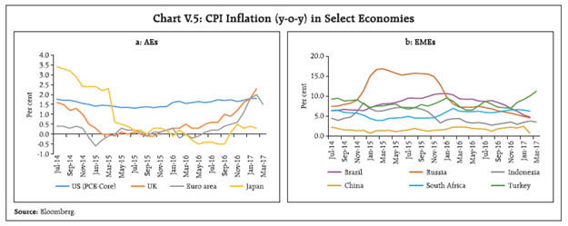
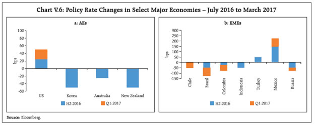 Inflation in major EMEs behaved divergently, driven by exchange rate movements and idiosyncratic factors. In China, Korea, Thailand and Indonesia, inflation remained low and well within the targets of central banks, despite some mild uptick in January due to food prices. In contrast, inflation ebbed in Brazil and Russia, helped by currency appreciation on the backdrop of recovery in commodity prices. In other major EMEs, inflation pressures remain a concern. In Turkey, high inflation trended further upward in recent months due to currency depreciation. High inflation has persisted in South Africa due to agricultural supply bottlenecks (Chart V.5b). V.3 Monetary Policy Stance Even though the monetary policy stance has generally remained accommodative globally, the stimulus provided through asset purchase programmes appears to have passed its peak. With incoming data showing strengthening of the US economy, the Federal Reserve raised the target federal funds rate twice in December 2016 and March 2017. The Federal Reserve expects economic conditions to evolve in a manner that warrant gradual increases in the federal funds rate. In contrast, the ECB extended the bond purchase programme to end-December 2017. For longer-lasting and smoother transmission of monetary stimulus, the extent of monthly purchases was reduced from 80 billion to 60 billion, while reducing the minimum maturity for bond purchases from two years to one year. The ECB has kept its policy rate unchanged since March 2016. The Bank of England has kept its monetary stance unchanged since the last easing effected in August in response to Brexit. The monetary stance was also left unchanged by the Bank of Japan (BoJ) in its meeting in March 2017. In major EMEs, the monetary policy stance has been driven by both domestic factors and the anticipation of a rate hike by the Federal Reserve. China raised its short term rates in March for the third time in three months. Turkey raised its policy rate in November to stem currency depreciation in the midst of domestic political uncertainty. Mexico raised its policy rate four times during November 2016 to March 2017 to counter currency depreciation and contain additional inflationary pressures arising from increase in gasoline prices by the government. In contrast, Brazil cut its policy rate four times between October 2016 and February 2017 to contain economic recession as inflationary pressure eased. Chile also reduced its policy rate in March 2017 (Chart V.6). In sum, monetary policy stance in EMEs has remained divergent. V.4 Global Financial Markets In a generally improving macroeconomic environment beginning in the second half of 2016, global financial markets were influenced by three events, viz., the US election, expectations and materialisation of the policy rate hike by the Federal Reserve, and uncertainty surrounding the Brexit roadmap. Sovereign bond yields in AEs rose further in Q4:2016. Expectations of fiscal stimulus and a quicker pace of normalisation in monetary policy led to a significant increase in US Treasury bond yields. Even as term premia increased, market-based measures of inflation compensation also contributed significantly to the rise in yields. In the Euro area, rising bond yields in late 2016 were boosted by the ECB’s decision to reduce the quantum of monthly purchase of assets and to resort to purchase of shorter-dated and loweryielding securities in December 2016. A rise in yield in the US also played a role in firming up of yields in the Euro area. Sovereign yields in the UK rose due to better than expected macroeconomic outcomes that obviated further monetary policy easing, and the rise in inflation following the sharp depreciation in the pound. In contrast, bond yields in Japan remained more or less flat at around zero as a result of active control of the yield curve by the Bank of Japan (Chart V.7a). 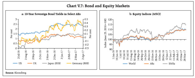 In emerging markets, bond yields behaved divergently. Yields rose in many EMEs after the US election, especially in countries with greater trade linkages with the US such as Mexico. In China, better economic performance and an uptick in inflation also partly fuelled a rise in long-term bond yields. In contrast, bond yields declined in Brazil as the central bank cut the policy rate to counter recession. Similarly, bond yields declined in Russia as recovery in oil prices and currency appreciation helped in moderating inflation expectations. The optimism generated after the US election, alongside the strengthening of the global recovery in the later part of 2016, led to a strong rally in global equity markets. The MSCI World Index, which measures global equity prices, increased by 9.7 per cent between November 1, 2016 and April 3, 2017. In the US, equity prices of financial sector companies registered the largest gains on prospects of less regulation of the sector and higher interest earnings due to rising bond yields. In the Euro area, the improving macroeconomic environment played a major role in the recovery of equity prices, helped by improvement in the financial position of some European banks. In the case of Japan, the depreciation of the yen, which boosted corporate earnings via better export earnings, played a major role. Equity prices in EMEs fell initially due to capital outflows and on concerns of increasing trade protectionism and rising borrowing costs. Subsequently, however, equity prices recovered in most EMEs as capital outflows ceased and then reversed, as the initial exuberance about the US economy subsided and the stance of the Federal Reserve turned less hawkish. In Brazil and Russia, the recovery in commodity prices also buoyed equity markets (Chart V.7b). Currency markets have been driven mainly by anticipation of policy initiatives by the new US administration and monetary policy stances in major AEs. The US dollar appreciated against most currencies beginning early November. It reached a 14-year high in December, before some reversal in Q1:2017 on uncertainty in realisation of Trump administration’s policy initiatives and expectations of a slower pace of rate hikes by the Federal Reserve. The euro depreciated against the US dollar on political uncertainty. The pound was volatile against the US dollar – it gained during late November and early December on expectations of a favourable deal with the EU, but depreciated in January 2017 on resurfacing of uncertainty in the deal. The Japanese yen depreciated as yield spreads between Japan and the US/Euro area widened, before narrowing somewhat in Q1 of 2017.  The currencies of EMEs have also depreciated sharply since November 2016. Central banks in several EMEs such as Mexico, Malaysia, Indonesia and Turkey intervened in currency markets to stem the depreciation, leading to losses of reserves. Despite intervention, the Mexican peso depreciated sharply due to its close trade and financial linkages with the US. The Turkish lira depreciated due to its domestic political problems. Initial depreciation of currencies in major commodity exporting EMEs such as Brazil, Russia and South Africa reversed, as the rise in commodity prices provided tailwinds (Chart V.8). Risk-on and risk-off behaviour and search for yields have been important drivers of portfolio flows in the recent period. During 2016, cross border capital flows were impacted mainly by the heightened uncertainty and abrupt political and policy changes. However, in the most recent period, portfolio flows have returned to EMEs, shrugging off the rise in interest rates in the US, as EMEs continue to provide attractive bond yields and return on equities. To sum up, the modest turnaround in global recovery since the latter part of the previous year is projected to strengthen further. While AEs are likely to consolidate economic recovery, the ongoing slowdown in EMEs could reverse. Despite some firming up, inflation in AEs is expected to largely remain stable going by the 1-year inflation swap rate in the US. Economic activity and financial markets will continue to be impacted by political and policy uncertainties as well as monetary policy moves by major AEs.
ABBREVIATIONS | ADR | American Depository Receipt | | AEs | Advanced Economies | | AIFIs | All India Financial Institutions | | AR | Autoregression | | ARIMA | Autoregressive Integrated Moving Average | | ARM | Additional Revenue Mobilisation | | BE | Budget Estimates | | BoJ | Bank of Japan | | BSE | Bombay Stock Exchange | | bps | Basis Points | | BVAR | Bayesian VAR | | BVARX | Bayesian VARX | | CASA | Current Account and Saving Account | | CBLO | Collateralised Borrowing and Lending Obligation | | CDs | Certificates of Deposit | | CGA | Controller General of Accounts | | CGST | Central Goods and Services Tax | | CI | Confidence Interval | | CII | Confederation of Indian Industry | | CLI | Composite Leading Indicator | | CMBs | Cash Management Bills | | CMIE | Centre for Monitoring Indian Economy | | CPB | Central Planning Bureau | | CPs | Commercial Papers | | CPC | Central Pay Commission | | CPI | Consumer Price Index | | CPI-AL | Consumer Price Index for Agricultural Labourers | | CPI-IW | Consumer Price Index for Industrial Workers | | CPI-RL | Consumer Price Index for Rural Labourers | | CRAR | Capital to Risk-weighted Assets Ratio | | CRR | Cash Reserve Ratio | | CSO | Central Statistics Office | | DGCI&S | Directorate General of Commercial Intelligence & Statistics | | DISCOMs | Distribution Companies | | ECB | European Central Bank | | ECBs | External Commercial Borrowings | | ECM | Error Correction Model | | EMDEs | Emerging Market and Developing Economies | | EMEs | Emerging Market Economies | | EU | European Union | | FAO | Food and Agriculture Organisation | | FBs | Foreign Banks | | FCCB | Foreign Currency Convertible Bond | | FCNR | Foreign Currency Non-Resident | | FDI | Foreign Direct Investment | | FICCI | Federation of Indian Chamber of Commerce and Industry | | FI | Financial Institution | | FIMMDA | Fixed Income Money Markets and Derivatives Association | | FIPB | Foreign Investment Promotion Board | | FMCG | Fast Moving Consumer Goods | | FOMC | Federal Open Market Committee | | FPI | Foreign Portfolio Investment | | FRBM | Fiscal Responsibility and Budget Management | | FR | Fixed Rate | | FY | Financial Year | | GARCH | Generalised Autoregressive Conditional Heteroscedasticity | | GDP | Gross Domestic Product | | GDR | Global Depository Receipt | | GFD | Gross Fiscal Deficit | | GFCE | Government Final Consumption Expenditure | | GFCF | Gross Fixed Capital Formation | | GFC | Global Financial Crisis | | GoI | Government of India | | GMM | Generalised Method of Moments | | GNDI | Gross National Disposable Income | | GNPAs | Gross Non-Performing Assets | | G-Secs | Government Securities | | GSDP | Gross State Domestic Product | | GST | Goods and Services Tax | | GVC | Global Value Chain | | GVA | Gross Value Added | | H1 | First Half of the Year | | H2 | Second Half of the Year | | HRA | House Rent Allowance | | ICRR | Incremental Cash Reserve Ratio | | IGARCH | Integrated Generalised Autoregressive Conditional Heteroscedasticity | | IGST | Integrated Goods and Services Tax | | IIP | Index of Industrial Production | | IOCL | Indian Oil Corporation Limited | | IPO | Initial Public Offering | | IMD | India Meteorological Department | | IMF | International Monetary Fund | | IND-AS | Indian Accounting Standard | | INR | Indian Rupee | | IRF | Impulse Response Function | | ISM | Institute for Supply Management | | JPC | Joint Plant Committee | | LAF | Liquidity Adjustment Facility | | LCR | Liquidity Coverage Ratio | | LIC | Life Insurance Corporation of India | | LPG | Liquefied Petroleum Gas | | M3 | Broad Money | | MA-SV | Moving Average Model with Stochastic Volatility | | mb/d | Million Barrels Per Day | | MCA | Ministry of Corporate Affairs | | MCLR | Marginal Cost of Funds Based Lending Rate | | MGNREGA | Mahatma Gandhi National Rural Employment Guarantee Act | | MOCI | Ministry of Commerce and Industry | | m-o-m | Month-on-Month | | MPC | Monetary Policy Committee | | MPR | Monetary Policy Report | | MSP | Minimum Support Price | | MSCI | Morgan Stanley Capital International | | MSMEs | Micro, Small and Medium Enterprises | | MSS | Market Stabilisation Scheme | | MVK | Multivariate Kalman Filter | | NABARD | National Bank for Agriculture and Rural Development | | NBFCs | Non-Banking Financial Companies | | NBFCs-D | Deposit-taking NBFCs | | NBFCs-ND-SI | Systemically Important Non-deposit Taking NBFCs | | NCAER | National Council of Applied Economic Research | | NDTL | Net Demand and Time Liabilities | | NDS-CALL | Negotiated Dealing System-Call | | NEER | Nominal Effective Exchange Rate | | NFC | Non-Food Credit | | NIM | Net Interest Margin | | NOAA | National Oceanic and Atmospheric Administration | | Non-IT | Non-Information Technology | | NPA | Non-performing Asset | | NSDL | National Securities Depository Limited | | OECD | Organisation for Economic Co-operation and Development | | OMOs | Open Market Operations | | OPEC | Organisation of the Petroleum Exporting Countries | | OROP | One Rank One Pension | | PADO | Public Administration, Defence and Other Services | | PCE | Partial Credit Enhancement | | PCE | Personal Consumption Expenditure | | PC | Phillips Curve | | PFCE | Private Final Consumption Expenditure | | PMI | Purchasing Managers’ Index | | POL | Petroleum, Oil and Lubricant | | PPAC | Petroleum Planning and Analysis Cell | | PSBs | Public Sector Banks | | PVBs | Private Sector Banks | | q-o-q | Quarter-on-Quarter | | RBI | Reserve Bank of India | | RE | Revised Estimates | | REER | Real Effective Exchange Rate | | RHS | Right Hand Side | | RMSEs | Root Mean Square Errors | | RRBs | Regional Rural Banks | | RW | Random Walk | | SAAR | Seasonally Adjusted Annualised Rate | | SAE | Second Advance Estimates | | SBNs | Specified Bank Notes | | SCBs | Scheduled Commercial Banks | | SDLs | State Development Loans | | SEBI | Securities and Exchange Board of India | | SLR | Statutory Liquidity Ratio | | SUT | Supply and Use Table | | T-Bill | Treasury Bill | | TRAI | Telecom Regulatory Authority of India | | TVW | Time Varying Weights | | TV-GDW | Time Varying Geometrically Backward Decaying Weights | | UDAY | Ujwal DISCOM Assurance Yojana | | UK | United Kingdom | | US | United States | | USD | US Dollar | | VAR | Vector Autoregression | | VR | Variable Rate | | VARX | Vector Autoregression Model with One Exogenous Variable | | WACR | Weighted Average Call Money Rate | | WALR | Weighted Average Lending Rate | | WADTDR | Weighted Average Domestic Term Deposit Rate | | WAR | Weighted Average Rate | | WPI | Wholesale Price Index | | WTI | West Texas Intermediate | | WTO | World Trade Organisation | | y-o-y | Year-on-Year | |