This article evaluates the annual gross domestic product (GDP) growth projections of the Reserve Bank of India (RBI) against final official estimates of GDP, which are normally released with a lag of about three years. During 1998-99 to 2016-17, on an average, growth projections underestimated realised growth. Forecast errors, committed in both directions, were free of any systematic bias, and remained modest in a cross-country context. Introduction For the conduct of monetary policy, central banks devote considerable time and resources to generate reliable forecasts of key macro-economic variables. Realised outcomes, however, often deviate from forecasts, leading to forecast errors. Assessment of forecast errors enables policy makers to recognise biases in forecasts, if any, and thereby helps in more informed and better decision-making (Lees, 2016). Historical forecast errors provide a reference for assessing uncertainty surrounding projections (Nakamura and Nagae, 2008). Error assessment can help mitigate the risk of policy mistakes which, in turn, can contribute to enhanced credibility (Binette and Tchebotarev, 2017). Given the significance of forecasts to policy making, a number of central banks across the world, both advanced and emerging market economies, regularly track forecast performance and emphasise incorporation of learnings from past errors in forecasting exercises. In India, literature on the assessment of forecast performance of key macro-economic variables is limited. A study specifically assessed the Reserve Bank’s forecast performance of the headline inflation for identifying the episodes of large forecast errors and understanding the underlying factors [Raj, et. al. (2019)]. In a related study, attempt has been made to examine the accuracy of median forecasts of Professional Forecasters’ (SPF) relative to official actual data on growth and inflation [Bordoloi, et. al. (2019)]. In a cross-country setting, another study analysed the inflation and GDP growth forecasts of 17 select central banks (including RBI) for 2018 and 2019 in a panel regression framework and sought to examine the determinants of growth forecast errors (RBI, 2020). No study, however, has made an assessment of the performance of the Reserve Bank’s growth forecasts vis-à-vis the final GDP estimates that is released by the Central Statistics Office1 (CSO) after a lag of about three years. This article seeks to bridge this gap. In particular, it investigates two issues: whether forecast errors have any systematic bias and are auto-correlated; and whether forecast performance improves with the flow of new information that are incorporated in revised GDP growth forecasts. The article is structured in four sections. Section II briefly covers literature review on the area, while data and methodology issues are discussed in Section III. Section IV presents the empirical findings. Section V sums up the discussions. II. Review of Literature The field of forecast evaluation was pioneered by Henri Theil (Mincer and Zarnowitz, 1969). In the last one decade or so, research interest in forecast accuracy assessment has gained momentum. Many central banks2 (particularly in the advanced economies and also in a few EMEs), and multilateral institutions such as the International Monetary Fund (IMF), the World Bank, the Organisation for Economic Co-operation and Development (OECD) have started assessing and discussing in public their forecast performance on key macro-economic variables, mainly real GDP growth and inflation. Most of these assessments, however, have predominantly been done for inflation forecasts. Researchers have also assessed the forecasting performance of multilateral institutions. Hong and Tan (2014) assessed the forecast performance of the UN, the IMF and the World Bank in respect of global growth and individual country growth for the period 2000-2012. They found that the forecasting performance of the UN was marginally better than that of the IMF and the World Bank at the global as well as country-group levels. Research in this area has also focused on comparing the forecasts of multilateral institutions with forecasts generated by other institutes [Oller and Barot (2000); Lees, op. cit.]. Oller and Barot, op. cit. analysed the performance of GDP growth and inflation as forecasted by the OECD and the respective national institutes of 13 European countries. They found that inflation forecasts were significantly more accurate than growth forecasts. They found no significant difference in forecast accuracy of the OECD and the institutes. Lees, op. cit. analysed the performance of the Reserve Bank of New Zealand’s forecasts (one-year and two-year ahead forecasts) during 2009 to 2015 in respect of a number of variables such as GDP growth, inflation, interest rates and the nominal exchange rate and compared it with the forecasts made by external forecasters. He reported that the Reserve Bank of New Zealand outperformed the median forecast for output growth. He did not find any evidence of bias in the Reserve Bank’s one-year ahead GDP growth forecasts but the mean two-year ahead error was relatively high at 0.48. Chang and Hanson (2015) analysed the forecasts made by the Board of Governors of the Federal Reserve System for a number of macro-economic variables, besides GDP, from 1997 to 2008. They found that forecasts of the Federal Reserve System significantly outperformed benchmark forecasts for horizons of less than one-quarter ahead. However, the accuracy of such forecasts weakened for the one-year ahead horizon. An Independent Evaluation Office (2015) assessed and compared the forecast performance of the Bank of England in respect of several variables such as growth, inflation, unemployment rate, wage growth, investment, house prices, etc., and compared it with private sector forecasts and the ECB. For UK GDP growth, it did not report any statistically significant evidence of bias. It also found that the accuracy of the Bank of England’s UK GDP growth forecasts compared favourably with that of the UK private sector forecasts, and other central banks, particularly at the one-year ahead horizon. Binette and Tchebotarev, op. cit. assessed the quality of annual GDP growth forecasts (annual and two-years ahead projections) made by the Bank of Canada for the period 1997 to 2016 in respect of Canadian economy. They found that bias in the growth forecast was often statistically insignificant. III. Data and Methodology The Reserve Bank has been publishing its GDP growth projections in the monetary policy statements. Till August 2016, the growth projections were published in the Governor’s policy statement. Since then, with the constitution of the Monetary Policy Committee (MPC) in September 2016, growth projections are published in the resolution of the MPC. The Monetary Policy Report (MPR), being published bi-annually from September 2014, also provides growth projections. In the present study, annual growth projections3 made by the Reserve Bank in its annual (April) and mid-term review policy statements (September / October / November) from 1998-99 onwards, as sourced from the Reserve Bank website, are considered. It is pertinent to mention that till 2004-05, only two policy statements were published – one in April/ May (Annual Policy Statement) and the other in September/ October/ November (Mid-term Review). From 2005-06 to 2009-10, four policy statements were published in a year. From 2010-11 to 2013-14, eight policy statements were announced in a year with the introduction of mid-quarter reviews. From April 2014, six bi-monthly monetary policy statements are being released every year. Annual realised growth numbers (final estimates) for the respective years are sourced from the CSO’s website. CSO’s final estimates4, which are updated using latest available data, provide the most accurate assessment of economic activity. So far, the CSO has published final GDP estimates only upto 2016-17. Hence, this study uses GDP data for the period from 1998-99 to 2016-17. Forecast error (Et) for a variable, say growth ‘X’, at time ‘t’ is measured as deviation of forecasted value (Ft) from the actual (observed) value (At). Thus, a negative mean forecast error shows that forecasted growth, on an average, exceeds the realised growth and represents over-prediction. In contrast, if the forecasted values, on an average, are lower than the actual growth, then it is a case of under-prediction. The performance on forecasting can be assessed by aggregating these forecast errors (Et) over a period using various statistical measures, which, inter alia include mean forecast error (MFE) and root mean square forecast error (RMSE). While average error or MFE is a measure of bias, the RMSE is a measure of accuracy. Mathematically, MFE is defined as follows: One of the weaknesses of MFE is that it may unduly get influenced by outliers. RMSE is defined as follows: RMSE is a widely used measure of forecast accuracy. A desirable property of an efficient forecast is that its errors should remain unbiased, which implies that over a considerable period of time, a forecaster would make positive errors as often as negative errors. Another desirable property of an efficient forecast is that the forecast error should not be autocorrelated (i.e., correlated with its past values). Both the properties of an optimal forecast can be assessed through regression estimates. Forecast error (Et) is said to be unbiased when the value of intercept (α) in the following regression is equal to zero (equation 4): The absence of biasedness and autocorrelation in forecast errors is attributed as ‘weak form informational efficiency’ and regarded as rational forecasting in the limited sense of McNees (1978) [Oller and Barot, op. cit.]. Forecast error (Et) would satisfy both the properties of unbiasedness and uncorrelatedness when the value of intercept (α) and the coefficient of one-period lagged term of forecast error estimates (β) are both equal to zero in the following regression (equation 5): where, i = 1 or 2 depending on whether growth forecast is made in annual policy statement (APS) and mid-term review (MTR), respectively. An efficient forecast should generate coefficients: α = 0 and β = 1. Furthermore, rejection of F-test of joint null hypothesis indicates inefficiency of forecasts. This study uses equation (6) to assess the quality of GDP forecast by the Reserve Bank utilising data on annual growth projections made by the Reserve Bank in its APS (in April/ May) and MTR (in September/ October/ November) and realised growth, which, published by the CSO, comes with a significant lag. The first estimate of GDP for a fiscal year is released by the CSO towards the fag end of the fiscal, i.e., at end-February, which undergoes further three rounds of sequential revision and the final GDP estimate of a year is available after a lag of 2 years and 10 months post the completion of the fiscal. Growth numbers, here, are based on real gross domestic product (GDP) at factor cost (erstwhile headline growth number), which was used as a reference for gauging economic activity. From 2012-13 onwards, the new headline GDP – real GDP at market price has been considered5. IV. Evaluation of Forecast Performance Magnitude and Variability Descriptive statistics of the forecast errors (i.e. deviation of realised figure from the forecast) for the period from 1998-99 to 2016-17 suggests under-prediction of GDP growth, on an average, for the entire period. Forecast errors, both of APS and MTR, are found to be normally distributed (Table 1). Comparatively, mean forecast errors of mid-term reviews were larger in magnitude. Mean forecast error of the MTR was, however, found to have lesser volatility than that of the APS. This is in line with the property of an optimal forecast that variance of forecast error should decline with availability of more information (Timmermann, 2006). An analysis of forecast errors for various years suggests that errors for both the APS and MTR have occurred on both the sides suggesting instances of both under-estimation and over-estimation (Charts 1.a and b). | Table 1: Descriptive Statistics of Growth Forecast Errors | | (1998-99 to 2016-17) | | | Annual Policy (APS) | Mid-term Review (MTR) | | Mean | 0.26 | 0.53 | | Median | 0.40 | 0.68 | | Maximum | 2.59 | 2.59 | | Minimum | -2.60 | -2.10 | | Std. Dev. | 1.62 | 1.27 | | Skewness | -0.31 | -0.35 | | Kurtosis | 1.95 | 2.37 | | Jarque-Bera Statistics (p-value) | 0.56 | 0.70 | | Source: Author's calculations. |
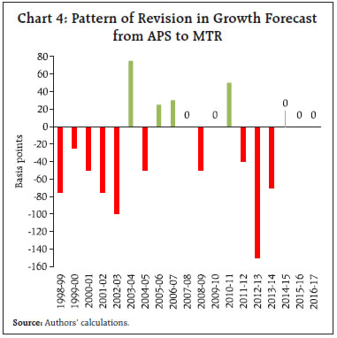
However, on an average, forecasted growth figures for both APS and MTR were found to be under-estimates; the instances of under-prediction was higher in the case of the latter (Chart 2). Higher frequency of under-prediction was found to persist for the MTR forecast errors even after excluding the drought years (Chart 3). As per the pattern of revision of growth forecasts from APS to MTR, the instances of downward revisions in growth forecasts outweighed the upward revisions (Chart 4). Forecast error, as measured by RMSE, using CSO’s realised growth and growth projections by the RBI in its APS for 1998-99 to 2016-17, was estimated at ± 1.60 per cent for the longer horizon (Table 2). For G-7 central banks, Bloomberg (2018) reported growth forecast errors in the range of 1.8 to 3.1 percentage points in respect of central banks of Japan, Euro Area, Canada, USA, and England for period 2006 to 2016 (Table 3). 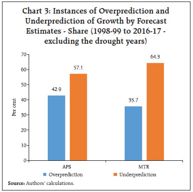
 The forecast error for annual growth projections made by the the Reserve Bank is observed to shrink as one moves from APS to MTR, as the latter incorporates more incoming information for generating forecasts. RMSE of the growth projections for the period from 1998-99 to 2016-17 was estimated to reduce from ± 1.60 per cent for the APS projections to ± 1.35 per for the MTR projections.6 It may also be noted that since the signing of Monetary Policy Framework Agreement between the Government of India and the Reserve Bank in February 2015 and adoption of flexible inflation targeting (FIT) framework, the RMSE of growth projection for 2015-16 to 2016-17 is found to decline. Nevertheless, it may be too early to make a judgement whether forecasting errors have got reduced in the post-FIT regime. Furthermore, the ratio of RMSE over the standard deviation of the realised growth (a metric of forecaster’s performance in relation to variability of the forecasted variable) also suggests that the ratio declines as one moves from APS to MTR. This again highlights that when more information becomes available for the economy as the year progresses, growth forecast error gets reduced. This is in line with the studies conducted in respect of other economies such as the USA, and Iceland [Binette and Tchebotarev, op. cit.7, Danielsson (2008)8]. | Table 2: RBI’s Forecast of Annual Growth Projections: Estimates of Error | | | MFE | RMSE | Std. Dev. (Realised Growth) | RMSE / Std. Dev. (Realised Growth) | | Annual policy statement | Mid-term review | Annual policy statement | Mid-term review | Annual policy statement | Mid-term review | | 1998-99 to 2006-07 | 0.23 | 0.51 | 1.78 | 1.46 | 1.98 | 0.90 | 0.74 | | 2007-08 to 2016-17 | 0.29 | 0.55 | 1.45 | 1.30 | 1.16 | 1.25 | 1.12 | | 2013-14 to 2014-15 | 1.30 | 1.65 | 1.43 | 1.67 | 0.50 | 2.86 | 3.34 | | 2015-16 to 2016-17 | 0.30 | 0.30 | 0.32 | 0.32 | 0.00 | - | - | | 1998-99 to 2016-17 | 0.26 | 0.53 | 1.60 | 1.35 | 1.63 | 0.98 | 0.82 | Note: MFE – Mean Forecast Error; RMSE – Root Mean Square Forecast Error.
Source: Authors’ calculations. |
| Table 3: Forecast Error Based on Average Squared Forecast Error Between 2006 and 2016 For Select Advanced Countries | | Country/ Region | Agency | Forecast error | | USA | Federal Reserve Board | 2.14 | | Canada | Bank of Canada | 2.27 | | Euro Area | European Central Bank | 2.86 | | England | Bank of England | 1.83 | | Japan | Bank of Japan | 3.11 | Note: Based on Central Bank GDP forecast one-year ahead.
Source: Bloomberg (2018). |
A comparison of the scatter plot of realised growth with the forecasts made in APS and MTR also suggests lower dispersion for the MTR as compared to APS, implying reduction in forecast error as the forecast horizon shrinks and more information becomes available for assessing the economic condition (Chart 5). For testing the unbiasedness property of forecast estimates, equation 4 (as discussed in Section III) was estimated using OLS estimation. If α is significantly different from zero, then the forecasts are said to be biased. The intercept was not found to be significantly different from zero for the forecast errors of the APS and the MTR at 5 per cent level of significance (Table 4). | Table 4: OLS Regression | | (Forecast error regressed on intercept) | | | Annual Policy | Mid-term Review | | Full Period (1998-99 to 2016-17) | 0.26
(0.37) | 0.53*
(0.28) | | 1998-99 to 2006-07 | 0.24
(0.70) | 0.51
(0.53) | | 2007-08 to 2016-17 | 0.29
(0.35) | 0.55*
(0.25) | Notes: 1. ***, **, & *: denote statistical significance at 1%, 5%, & 10%, respectively.
2. Figures in parentheses are standard errors.
3. Heteroscedasticity and autocorrelation consistent (HAC) standard errors. | For testing, the unbiasedness and non-autocorrelation properties of the forecast estimates, following equation 5 framework, forecast error series was regressed on intercept and its one-period lag, using APS and MTR data separately. Regression results based on equation 5 suggest that coefficients of the lag term as also the intercept are statistically insignificant, validating no biasedness or auto-correlation in forecast errors (Table 5). To reaffirm unbiasedness, whether or not forecast errors followed the same pattern during the drought years was also examined. For the drought years 2002-03 and 2015-16, the Reserve Bank’s GDP growth forecast was found to have exceeded the actual outcome (over prediction), while for another spell of drought years in 2004-05, 2009-10 and 2014-15, GDP growth forecasts were lower than the realised growth (under prediction) (Chart 6). This implies that even in abnormal years, forecast errors were neither biased and nor skewed. | Table 5: OLS Regression | | (Dependent Variable – Forecast Error) | | | Annual Policy | Mid-term Review | | Constant | 0.28
(0.41) | 0.55
(0.34) | | Forecast Errort-1 | 0.01
(0.25) | -0.05
(0.25) | | Diagnostics | | | | Adj. R2 | -0.06 | -0.06 | | Prob. (Jarque-Bera statistics) | 0.53 | 0.65 | | Prob (BGSLM test F-stats) | 0.78 | 0.66 | | Prob. (BPG F-test) | 0.41 | 0.95 | Notes: 1. ***, **, & *: denote statistical significance at 1%, 5%, & 10%, respectively.
2. Figures in parentheses are heteroscedasticity and autocorrelation consistent (HAC) adjusted standard errors.
3. BGSLM - Breusch-Godfrey Serial Correlation Lagrange Multiplier; BPG - Breusch-Pagan-Godfrey. |
How good is the quality of growth forecast? Another metric for assessing the quality of forecast is through understanding the extent of association between forecast figures and realised values. For the same, Mincer-Zarnowitz regression is employed, which involves regressing the realised values of a variable on a constant and its forecast. Mincer-Zarnowitz (MZ) regression (as in equation 6) was estimated separately for the annual GDP growth forecast made in the APS and the MTR. Results suggest that bias is not significantly different from zero. Secondly, the coefficients of forecasts for AP and MTR were found to be statistically significant. Wald test with the null hypothesis of slope coefficients being equal to unityfor both the equations was not rejected implying one-to-one correspondence between forecasted growth and actual growth (Table 6). The slope coefficient for the MTR equation is much higher than that of the slope coefficient for the APS equation and very close to one. Furthermore, the R2 of the regression increases from 0.06 to 0.39 as one moves from APS to MTR. The findings confirm that the growth forecast performance of the Reserve Bank is good and improves with availability of more information. Further, F-test did not reject null hypothesis of α = 0 and β = 1 for both APS and MTR, which validates that the Reserve Bank’s growth forecasts are efficient. Also, the forecast errors get reduced as more information becomes available on various macro-economic indicators. Table 6: OLS Regression
(Mincer-Zarnowitz Regression) (Dependent Variable – Realised growth) | | | Annual Policy | Mid-term Review | | Constant | 2.95
(2.39) | 0.74
(2.00) | | Forecasted Growth | 0.62*
(0.32) | 0.97**
(0.28) | | Diagnostics | | | | Adj. R2 | 0.06 | 0.39 | | Durbin Watson stats. | 1.72 | 2.07 | | Prob. (Jarque-Bera statistics) | 0.53 | 0.75 | | Prob. (BGSLM test F-stats) | 0.43 | 0.94 | | Prob. (BPG F-test) | 0.52 | 0.29 | | Joint F-test (α = 0; β = 1) (p-value) | 0.45 | 0.18 | Notes: 1. ***, **, & *: denote statistical significance at 1%, 5%, & 10%, respectively.
2. Figures in parentheses are heteroscedasticity and autocorrelation consistent (HAC) adjusted standard errors.
3. BGSLM - Breusch-Godfrey Serial Correlation Lagrange Multiplier; BPG - Breusch-Pagan-Godfrey. | Directional Accuracy A good forecast correctly tracks the turning points of business cycles. For measuring directional accuracy, the ‘hit ratio’, which indicates how often a forecaster correctly predicts an increase or a decrease in growth was calculated (Binette and Tchebotarev, op. cit.). Towards the start of forecast cycle when the annual policy was announced, forecast was found to correctly predict the change in sign of annual real GDP growth roughly 33 per cent of the time, which improves to about 67 per cent at the shorter forecast horizon for mid-term reviews (Chart 7). V. Conclusion Accuracy in forecasts of key macro-economic variables is of paramount importance to central banks for conducting forward-looking monetary policy. In India, final estimates of GDP, after several rounds of revisions, become available after a lag of two years and ten months. Currently, for example, final GDP numbers are available only for 2016-17. An assessment of annual GDP growth forecasts made by the Reserve Bank during 1998-99 to 2016-17 relative to the final estimates of the GDP suggests that growth forecast errors were relatively lower for MTR than that of the APS. Growth forecast errors were also not found to have any systematic bias. Mincer-Zarnowitz regression results suggest improved quality of forecast with improved capture of information in MTR. Under-prediction of GDP growth on an average was also observed. The directional accuracy of forecast estimates, viz., tracking of turning points, was also found to be better for the MTR than for the APS. References Anderson, Palle S. (1997). “Forecast Errors and Financial Developments”, BIS Working Papers No. 51, November. Binette, Andre and Dmitri Tchebotarev (2017). “Evaluating Real GDP Growth Forecasts in the Bank of Canada Monetary Policy Report”, Staff Analytical Note 2017-21, Bank of Canada. Bloomberg (2018). “Which Central Bank Is the Most Accurate Forecaster?”, Special Report – Central Banks, Q1: 2018, January 17. Bordoloi, Sanjib; Rajesh Kavediya; Sayoni Roy; and Akhil Goya (2019). “Changes in Macroeconomic Perceptions: Evidence from the Survey of Professional Forecasters”, RBI Bulletin, November. Chang, Andrew C. and Tyler J. Hanson (2015). “The Accuracy of Forecasts Prepared for the Federal Open Market Committee,” Finance and Economics Discussion Series 2015-062. Washington: Board of Governors of the Federal Reserve System. Danielsson, Asgeir (2008). “Accuracy in forecasting macroeconomic variables In Iceland”, Central Bank of Iceland Working Papers No. 39, May. Government of India, Ministry of Statistics and Programme Implementation, www.mospi.gov.in Hong, Pingfan and Zhibo Tan (2014). “A Comparative Study of the Forecasting Performance of Three International Organizations”, DESA Working Paper No. 133, June. Independent Evaluation Office (2015). “Evaluating forecast performance”, Bank of England, November. Lees, Kirdan (2016). “Assessing forecast performance”, Reserve Bank of New Zealand Bulletin, Vol. 79, No 10, June. McNees, S. K. (1978). “The ‘rationality’ of economic forecasts” American Economic Review 68(2), 301–305. Mincer, Jacob A. and Victor Zarnowitz (1969). “The Evaluation of Economic Forecasts”, in Mincer, Jacob A., (Ed.), Economic Forecasts and Expectations, NBER, New York. Nakamura, Koji and Shinichiro Nagae (2008). “The Uncertainty of the Economic Outlook and Central Banks’ Communications”, Bank of Japan Review, 2008-E-1, June. Oller, Lars-Erik and Bharat Barot (2000). “The accuracy of European growth and inflation forecasts”, International Journal of Forecasting, 16:293–315. Raj, Janak; Muneesh Kapur; Praggya Das; Asish Thomas George; Garima Wahi; and Pawan Kumar (2019). “Inflation Forecasts: Recent Experience in India and a Cross-country Assessment”, Mint Street Memo No. 19, Reserve Bank of India, May. Reserve Bank of India (2020). “Monetary Policy Report”, April. Reserve Bank of India, www.rbi.org.in Timmermann, Allan (2006). “An Evaluation of the World Economic Outlook Forecasts”, IMF Working Paper, WP/06/59, March.
|