Jeevan Kumar Khundrakpam
Sitikantha Pattanaik*
Contagion from the global crisis necessitated use of fiscal stimulus measures in India
during 2008-10 in order to contain a major slowdown in economic growth. Given the usual
downward inflexibility of fiscal deficit once it reaches a high level, as has been experienced
by India in the past, there could be medium-term implications for the future Inflation path,
which must be recognised while designing the timing and speed of fiscal exit. Inflation, at
times, may become effectively a fiscal phenomenon, since the fiscal stance could influence
significantly the overall monetary conditions. As highlighted in this paper, fiscal deficit
could be seen to influence the Inflation process either through growth of base money created
by the RBI (i.e. net RBI credit to the Government) or through higher aggregate demand
associated with an expansionary fiscal stance (which could increase growth in broad
money). Empirical estimates of this paper conducted over the sample period 1953-2009
suggest that one percentage point increase in the level of the fiscal deficit could cause about
a quarter of a percentage point increase in the Wholesale Price Index (WPI). The paper
emphasises that the potential Inflation risk should work as an important motivating factor
to ensure a faster return to the fiscal consolidation path in India, driven by quality of
adjustment with appropriate rationalisation of expenditure, rather than waiting for revenue
buoyancy associated with sustained robust growth to do the job automatically. The
importance of fiscal space in the India specific context needs to be seen in terms of not only
the usual output stabilisation role of fiscal policy but also the occasional need for use of
fiscal measures to contain such Inflationary pressures that may arise from temporary but
large supply shocks.
JEL Classification : B21, E31, E62.
Keywords : Crisis, Fiscal, Inflation.
Introduction
Fiscal stimulus emerged as the key universal instrument of hope in
almost every country around the world, when the financial crisis in the
advanced economies snowballed into a synchronised global recession.
Borrowing as much at as low a cost as possible to stimulate the sinking
economies necessitated unprecedented coordination between the fiscal
and monetary authorities. It is the fiscal stance of the Governments
that had to be accommodated without any resistance by the monetary
authorities so as to minimise the adverse effects of the crisis on output
and employment, while also saving the financial system from a complete
breakdown. Given the deflation concerns in most countries –rather than
the fear of Inflation – monetary authorities had no reasons to resist. The
universal resort to fiscal stimulus, however, has now led to significant
increase in deficit and debt levels of the advanced economies, which
may operate as a permanent drag for some time, vitiating the overall
macroeconomic outlook, including Inflation. OECD projections indicate
that OECD level fiscal deficit may reach 60 year high of about 8 per
cent of GDP in 2010, and public debt may exceed 100 per cent of GDP
in 2011, which will be 30 percentage points higher than the comparable
pre-crisis levels in 2007. In the process of managing the financial crisis,
fiscal imbalances have been allowed to reach levels that could trigger
fiscal crisis in several countries. The market perception of sovereign
risk has changed significantly in 2010, particularly since the time that
the fiscal crisis in Greece has surfaced and contaminated the Euro-area.
The same private sector that was bailed out at the cost of fiscal excesses
will now perceive Government papers as risky and fiscal imbalances as
the harbinger of the next crisis.
In India, the fiscal response to the global crisis was swift and
significant, even though India clearly avoided a financial crisis at home
and also continued to be one of the fastest growing economies in the
World in a phase of deep global recession. Despite the absence of any
need to bailout the financial system, it is the necessity to partly offset the
impact of deceleration in private consumption and investment demand
on economic growth, which warranted adoption of an expansionary fiscal
stance. One important consequence of this, though, was the significant deviation from the fiscal consolidation path, and the resultant increase
in the fiscal deficit levels over two consecutive years (2008-10).
The immediate impact of the higher levels of fiscal deficit on
Inflation in India could be seen as almost negligible, since: (a) the
expansionary fiscal stance was only a partial offset for the deceleration
in private consumption and investment demand, as the output-gap
largely remained negative, indicating no risk to Inflation in the nearterm;
and (b) despite large increase in the borrowing programme of
the Government to finance the deficit, there was no corresponding
large expansion in money growth, since demand for credit from the
private sector remained depressed. Thus, neither aggregate demand
nor monetary expansion associated with larger fiscal deficits posed any
immediate concern on the Inflation front. The usual rigidity of deficit
to correct from high levels to more sustainable levels in the near-term,
however, entails potential risks for the future Inflation path of India,
which may become visible when the demand for credit from the private
sector reverts to normal levels and if the revival in capital flows turns
into a surge again over a sustained period, that may require sterilised
intervention. The major risk to future Inflation would arise from how
the extra debt servicing could be financed while returning to sustainable
levels through planned consolidation. Revenue buoyancy associated
with the recovery in economic activities to a durable high growth path
would only contribute one part; the major important part, however, has
to come either from a combination of higher taxes, withdrawal of tax
concessions and moderation in public expenditure, which could weaken
growth impulses or from higher Inflation tax, suggesting higher money
growth and associated pressure on future Inflation.
Conceptually, the risk to Inflation from high fiscal deficit arises
when fiscal stimulus is used to prop up consumption demand, rather
than to create income yielding assets through appropriate investment,
which could have serviced the repayment obligations arising from
larger debt. As highlighted by Cochrane (2009) in the context of the
US, “...If the debt corresponds to good quality assets, that are easy...If
the new debt was spent or given away, we’re in more trouble. If the debt
will be paid off by higher future tax rates, the economy can be set up for a decade or more of high-tax and low-growth stagnation. If the Fed’s
kitty and the Treasury’s taxing power or spending-reduction ability are
gone, then we are set up for Inflation.” It may be worth recognising that
all over the world, at some stage, the risk of active anti-Inflationary
policy conflicting with inflexible fiscal exit cannot be ruled out. As
highlighted by Davig and Leeper (2009) in this context for the US,
“...as Inflation rises due to the fiscal stimulus, the Federal Reserve
combats Inflation by switching to an active stance, but fiscal policy
continues to be active....In this scenario, output, consumption and
Inflation are chronically higher, while debt explodes and real interest
rates decline dramatically and persistently”.
The future risks to Inflation in India from fiscal stimulus, thus could
arise from the downward inflexibility of the deficit levels, and with
revival in demand for credit from the private sector and consolidation
of growth around the potential, the fiscal constraint could be manifested
in the form of pressures on both aggregate demand and money supply.
Surges in capital flows could complicate the situation further. This paper
recognises the possible policy challenge arising from higher money
growth on account of persistent fiscal constraint, revival in private credit
demand and surges in capital flows, on the one hand, and higher policy
interest rate chasing higher Inflation on the other. Possible crowding-out
effects associated with the fiscal constraint may also lead to a situation
where high Inflation and high nominal interest rates co-exist. Since
much of these possibilities could be empirically validated over time
depending on what outcome actually may materialise in the future, this
paper not only recognises the potential risks to the future Inflation path,
but also aims at unravelling the relevance of the perception by studying
the relationship between fiscal deficit and Inflation in India over the
sample period 1953 to 2009.
Macroeconomic variables are generally interrelated in a complex
manner. Therefore, a deeper understanding of Inflation dynamics would
involve analysing its relationship with macroeconomic variables such
as deficit, money supply, public debt, external balance, exchange rate,
output gap, global Inflation and commodity prices, and interest rates.
In the literature, particularly in the developing country context, simple models are, however, often used to analyse the Inflationary impact of
fiscal deficit. This largely reflects the role of fiscal dominance, which
has often been a phenomenon in many developing countries. Thus,
fiscal-based theories of Inflation are more common in the literature of
developing countries (for example, Aghevli and Khan (1978), Alesina
and Drazen (1978) and Calvo and Vegh (1999)). On the other hand, for
developed countries, fiscal policy is often considered to be unimportant
for Inflation determination, at least on theoretical grounds, as the desire
to obtain seigniorage revenue plays no obvious role in the choice of
monetary policy (Woodford, 2001).
In the Indian context also, there are several studies analysing the
nexus between government deficits, money supply and Inflation. The
findings of these studies generally point to a self perpetuating process
of deficit-induced Inflation and Inflation-induced deficit, besides the
overall indication that government deficits represent an important
determinant of Inflation (for example, Sarma (1982), Jhadav (1994) and
Rangarajan and Mohanty (1998)). The above results have been on the
expected lines given that till the complete phasing out of the ad hoc
treasury bills in 1997-98, a sizable portion of the government deficit
which could not be financed through market subscription was monetised.
However, extending the period of analysis further beyond the automatic
monetisation phase, Ashra et al (2004) found no-long relationship
between fiscal deficit and net RBI credit to the Government and the
latter with broad money supply. Thus, they concluded that there is no
more any rationale for targeting fiscal deficit as a tool for stabilisation.
On the other hand, Khundrakpam and Goyal (2009), including more
recent data and adopting ARDL approach to cointegration analysis,
found that government deficit continues to be a key factor causing
incremental reserve money creation and overall expansion in money
supply, which lead to Inflation.
In this paper, we use a simple model to study the Inflationary
potential of fiscal policy in India by estimating the long-run relationship
and the short-run dynamics between fiscal deficit, seigniorage and
Inflation. The motivation is that fiscal deficit can lead to Inflation either
directly by raising the aggregate demand (demand pull Inflation), or indirectly through money creation, or a combination of both. Against
this background, Section-II presents the challenges associated with
fiscal exit for advanced economies as well as EMEs, and highlights
the issues that are particularly important for India. Section III explains
briefly the analytical framework employed in the paper. In section IV, the
estimation procedures are explained. The data and empirical results are
analysed in section V. Section VI contains the concluding observations.
Section II
The Challenge of Fiscal Exit – What is Important for India?
The unprecedented stimulus that was used across countries to avert
another Great Depression is widely believed to have shown the seeds
of the next crisis. Public debt levels in the advanced economies are
projected to explode to levels never seen during peace-time, leaving
almost no fiscal space for managing other shocks to the economies
in future, besides significantly constraining normalisation of overall
macroeconomic conditions. Some of the projected debt figures look
uncomfortably high – revealing in true sense the trade-offs involved
in policy options. A better today ensured through policy interventions
could enhance risks for the future. In the case of sub-prime crisis, the
impact on the world economy will be permanent and is expected to
persist over several decades through the channel of high public debt.
What then is the dimension of the challenge we are facing today? IMF
projections indicate that in the G-20 advanced economies, Government
debt would reach 118 per cent of GDP in 2014, which will be 40 per
cent higher than the pre-crisis levels. Consolidating the level to about
60 per cent of GDP by 2030 would require raising the average structural
primary balance by 8 per cent of GDP, which is not easy, though not
impossible. But this order of adjustment will involve other costs. One
could first see why the adjustment options may not be easy, and then,
what other costs could result from sustained high levels of public debt.
Why Debt Normalisation could be Difficult?
Many of the advanced economies were preparing their fiscal
conditions to face the challenges associated with demography when the crisis unfolded. The pressure from demography on the fiscal conditions
in terms of social security needs and aging population will increase
over time, whereas the crisis will leave behind additional pressure
arising from the impact of lower potential output and patchy recovery
on revenues and from high unemployment and jobless recovery on
expenditure. Collapse in asset prices also seems to have affected the
funded part of the social security systems. The plausible options for debt
normalization include higher taxes, higher economic growth and the
associated revenue buoyancy, lower expenditure or use of Inflation tax.
Many of the advanced economies already have higher tax/GDP ratios,
and future increases in tax rates may also affect growth. Moreover,
in a globalised world, higher taxes could shift economic activities to
other parts of the world. Lower expenditure, given the constraint of
aging population and high unemployment, and higher debt servicing
associated with the higher debt, could be Difficult. Higher economic
growth, thus, could be the best possible option. Search for new sources
of growth would be a key policy challenge, which has to be also seen in
relation to the rising prominence of EMEs in the global economy and the
competition they would provide in the search for higher productivity.
The Costs of Sustained High Levels of Public Debt
A critical part of the policy challenge associated with high public
debt is to recognize upfront the costs for the economy, without being too
alarmist. Some of the costs seem obvious, even though because of the
non-linearity in the relationships between key evolving macroeconomic
variables, it may not be easy to quantify them. Some of these obvious
costs could be:
(a) Lack of fiscal space to deal with future shocks, including future
downturns in business cycles.
(b) Pressure on interest rates and crowding-out of resources from the
private sector. This effect is not visible as yet because of weak
private demand and expansionary monetary policies. As private
demand recovers and monetary policy cycles turn around, potential
risks will materialize. Three specific channels could exert pressure
on the interest rate: (i) larger fiscal imbalances would imply lower domestic savings, (ii) increase in risk premia, as market would
differentiate between debt levels and expect a premium in relation
to the perceived risk, which is already evident after the experience
of Dubai World and Greece, and (iii) higher Inflation expectations
that would invariably result from high levels of debt, which will be
reflected in the nominal interest rates.
(c) Pressure on central banks to dilute their commitment to and focus
on price stability. In this context, one may see the Inflation tolerance
levels of central banks rising. The IMF’s argument that raising the
Inflation target in advanced economies from 2 per cent to 4 per cent
may not add significant distortions to the economies should also be
carefully examined by central banks. One must recognise why some
feel that return to pre-crisis levels of central bank independence
with focus on price stability would be critical to improve the future
macroeconomic conditions, given the large debt overhang. Price
stability will be critical to ensure high growth, which in turn can
effectively contribute to debt consolidation without imposing costs
of adjustments through other options. The extent of dilution of
central bank independence may also increase if financial stability is
made an explicit mandate of central banks.
How then to Approach Fiscal Exit?
In planning the approach to fiscal exit, the scope for any
complacency based on some misplaced arguments must be avoided.
One such argument could be “no threshold level of debt could be risky”,
given the experience of Japan, which has been operating with very high
levels of debt for quite some time. One cannot ignore the fact that in
Japan private demand has remained depressed for more than a decade,
and much of the debt of the government is held internally as part of
domestic savings. The second flawed argument could be that Dubai and
Greece type shocks cannot cause any systemic global concern since
these shocks are too insignificant for the global economy. The most
dangerous argument, though, could be to support “Inflation tax” as a
means to reduce the real debt burden, on the ground that the alternative
option of higher taxes could be equally distortionary. IMF estimates indicate that higher Inflation in advanced economies at about 6 per cent
maintained over five years could reduce the real debt burden by about
25 per cent (IMF, 2009).
The fiscal exit plans, thus, must involve clarity and commitment.
The broad contours of such strategies may have to emphasise: (a)
medium-term fiscal framework, (b) credible commitment, (c) adoption
of fiscal rules – with scope for deviations to deal with future shocks,
including cyclical slowdowns, and (d) clarity in communication.
Why Fiscal Exit in EMEs Could be Different?
EMEs entered the global crisis with much better fiscal space,
as fiscal discipline was seen generally as a critical aspect of sound
macroeconomic environment to support higher growth. Since the
financial sector of the EMEs did not require any official bailout, the
magnitude of fiscal support needed during the global crisis was also not
as high as in the advanced economies. More importantly, with stronger
recovery ahead of the advanced economies, EMEs can implement fiscal
exit faster without creating concerns for growth. Stronger recovery
in growth will also improve revenue buoyancy. EMEs have to be
particularly careful about fiscal exit, unlike in advanced economies,
since fiscal indiscipline has conventionally created other problems such
as high current account deficit, pressures on Inflation, crowding-out
concerns and even capital outflows. The fiscal exit challenges in EMEs,
thus, will be different from those in the advanced economies.
Fiscal Exit in India
India was on a sustained path of fiscal consolidation prior to the
global crisis, conditioned by the discipline embodied in the Fiscal
Responsibility and Budget Management (FRBM) Act, 2003. The
FRBM rules required phased reduction in fiscal deficit to 3 per cent of
GDP by end March-2009, with commitment to also eliminate revenue
deficit by that time. The progress on fiscal consolidation turned out to be
faster than initially expected, as high growth during the five year period
2003-08 ensured better revenue buoyancy. Fiscal deficit as percentage
of GDP fell from 4.5 per cent in 2003-04 to 2.6 per cent in 2007-08, leading to attainment of the target one year before what was initially
set under the FRBM rules in 2004. Revenue deficit also declined from
3.6 per cent of GDP to 1.1 per cent of GDP during the corresponding
period. The FRBM, thus, had created considerable fiscal space, led by
revenue buoyancy, when the impact of the global recession on domestic
activities warranted introduction of anti-crisis fiscal response. Some
have viewed the fiscal consolidation as a favourable macroeconomic
condition that contributed to India’s shift to the higher growth trajectory,
even though it is a fact that fiscal consolidation resulted primarily
because of high growth.
When the global crisis started to spread, despite perceptions of
decoupling and a sound financial system at home, there was a clear
risk of slowdown in Indian growth, which had to be arrested through
the appropriate policy response. Because of the heightened uncertainty,
and the “black swan” nature of the series of adverse developments
that unfolded after the bankruptcy of Lehman Brothers, the Indian
policy response had to be swift and significant, with a heavy accent
on adequate precaution. Two major fiscal decisions that were taken
earlier, i.e., the farm debt waiver scheme and the Sixth Pay Commission
award, worked like expansionary stimulus, where the decision lag was
almost zero, since the decisions had been taken and partly implemented
even before the crisis-led need for fiscal stimulus was recognised. The
subsequent crisis related fiscal stimulus was delivered in the form of tax
cuts as well as higher expenditure, dominated by revenue expenditure,
as the deceleration in private consumption expenditure turned out to
be significant, which needed to be partly offset by higher government
expenditure. Reflecting the expansionary fiscal stance – involving
a deliberate deviation from the fiscal consolidation path – the fiscal
deficit of the Central Government rose from 2.6 per cent of GDP in
2007-08 to 5.9 percent in 2008-09 and further to 6.7 per cent in 2009-10.
Even the State Governments, which were progressing well on fiscal
consolidation – driven partly by the incentives from the Twelfth Finance
Commission – experienced a setback to the process, resulting primarily
from pressures on revenues and central transfers associated with the
economic slowdown as well as the compelling demand to match the pay revision already announced for Central Government employees.
Gross fiscal deficit of the states, which had improved to 1.5 per cent of
GDP by 2007-08, expanded to 3.2 per cent of GDP in 2009-10.
The role of the expansionary fiscal stance adopted by both the
Central and the State Governments has to be seen in the context of
the fact that private consumption demand, which accounts for close
to 60 per cent of aggregate demand, exhibited sharp deceleration in
growth, from 9.8 per cent in 2007-08 to 6.8 per cent and 4.1 per cent
in the subsequent two years. Government consumption expenditure,
which accounts for just about 10 per cent of aggregate demand, had to
be stepped up significantly to partially offset the impact of the sharp
deceleration in the growth of private consumption demand. Reflecting
the fiscal stimulus, growth in government consumption expenditure was
as high as 16.7 per cent in 2008-09, as a result of which the contribution
of government expenditure to the overall growth in aggregate demand
rose almost three fold – from 10.4 per cent in 2007-08 to 33.6 per cent
in 2008-09. The fiscal stance, thus, had a clear role in arresting sharper
slowdown in economic growth.
Given the possibility of a weak fiscal position operating as a
drag on economic growth in the medium-run – through crowding-out
pressures, besides the scope for causing higher Inflation – the need for
faster return to fiscal consolidation path was recognised quite early in
India, which was articulated and emphasised by the Reserve Bank in
its policy statements, as signs of stronger recovery in growth started
to emerge. By the time the Budget for 2010-11 was announced in
February 2010, better evidence on broad-based momentum in recovery
created the space for gradual roll back of some of the fiscal measures
that were taken in response to the crisis. At the macro level, while gross
fiscal deficit has been budgeted lower at 5.5 per cent of GDP, net market
borrowing programme has also been scaled down by more than 10 per
cent. In terms of specific measures, some of the stimulus-led tax cuts
have been rolled back, greater non-tax revenue from disinvestments and
auction of 3-G/BWA spectrum has been realised and growth in non-plan
expenditure has been significantly curtailed to 4.1 per cent in 2010-11
from 26.0 per cent in the previous year, much of which will result from rationalisation of subsidies. More importantly, indicating the resolve to
return to the fiscal consolidation process, a Medium Term Fiscal Policy
Statement (MTFPS) has been issued along with plans for tax reforms,
both direct and indirect. As per the MTFPS, there will be annual rolling
targets for revenue deficit and gross fiscal deficit so as to reach 2.7
per cent and 4.1 per cent of GDP, respectively, by 2012-13. Goods and
Services Tax (GST) and Direct Tax Code (DTC), to be implemented
in 2011-12, will be critical components of the fiscal consolidation,
which could help in improving the tax to GDP ratio from 10.8 per cent
in 2010-11 to 11.8 per cent in 2012-13. Reflecting the planned fiscal
consolidation, total debt liabilities of the Central Government could
also be expected to moderate from 51.5 per cent of GDP in 2009-10 to
48.2 per cent of GDP in 2012-13. The Indian approach to fiscal exit – in
terms of both adoption of specific fiscal consolidation measures in sync
with the recovery and announcement of medium-term targets for phased
consolidation – reflects the recognition in the sphere of policy-making
of the importance of a disciplined fiscal environment for sustainable
high growth.
The quality of fiscal adjustment, however, must receive greater
attention, given the medium-term double digit growth objective. Like
the previous phase of fiscal consolidation during 2004-08, stronger
recovery in growth will improve revenue buoyancy. Moreover, given
the fact that a large part of the government borrowing (excluding the part
invested by FIIs) is financed domestically, the sovereign risk concerns
would also remain contained. These favourable aspects, however,
should not dilute the focus on consolidation from the expenditure side.
Even if gross fiscal deficit for 2010-11 has been budgeted to decline to
5.5 per cent of GDP from 6.7 per cent in the previous year, that may not
signal any major move in the direction of structural consolidation, if
one removes the one-off components from the revenue and expenditure
sides. Adjusted for disinvestment and 3-G/BWA auction proceeds on
the revenue side, and farm debt waiver and Sixth Pay Commission
arrears on the expenditure side, the reduction in gross fiscal deficit as
per cent of GDP would be much less, i.e. by 0.3 percent as against 1.2
percent envisaged in the Budget. The magnitude and quality of fiscal adjustment could have a significant conditioning influence on India’s
medium-term growth prospects.
In the absence of faster and better quality fiscal adjustment, at least
four major risks to macroeconomic conditions could be envisaged: (a)
the decline in domestic savings, led by the fall in public sector savings,
which will lower the potential output path, (b) higher overall interest
rates, when the revival in demand for credit from the private sector starts
competing with the borrowing programme of the government, (c) limit
the capacity to manage the exchange rate and the domestic liquidity
impact of possible surges in capital flows, since the use of sterilisation
options like the MSS could exert further pressures on the interest rates,
and thereby lead to even higher inflows, and (d) may even force reversal
of reforms, such as use of higher SLR requirements for banks or even
introduction of SLR for non-banking entities in the financial system
to create a captive market for the government borrowing programme.
These possible potential implications signify why fiscal discipline is
so critical in a market based economy. Often, in the search for easy
solutions, direct or indirect monetisation could be preferred, which in
turn could give rise to higher Inflation. This paper primarily highlights
the Inflation risks to India from the fiscal imbalance, and argues that
fiscal space is as critical for managing Inflation as for stabilising the
output path.
Section III
The Analytical Framework
Inflation, according to monetarists, is always and everywhere a
monetary phenomenon. Following the seminal contribution by Sargent
and Wallace (1981), however, it is viewed that fiscally dominant
governments running persistent deficits would sooner or later finance
those deficits through creation of money, which will have Inflationary
consequences. Fischer and Easterly (1990), thus, argue that rapid
monetary growth may often be driven by underlying fiscal imbalances,
implying that rapid Inflation is almost always a fiscal phenomenon.
Historical evidences have shown that governments often resorted
to seigniorage (or Inflation tax) during times of fiscal stress, which had Inflationary consequences. Thus, contemporary macroeconomic
literature, while trying to explain Inflationary phenomenon has also
focussed on the fiscal behaviour, particularly in the developing country
context. This is because fiscally dominant regimes are often seen as
a developing country phenomenon, due to less efficient tax systems
and political instability, which lead to short-term crisis management at
the cost of medium to long-term sustainability. As noted by Cochrane
(2009), “...Fiscal stimulus can be great politics, at least in the shortrun.”
Furthermore, more limited access to external borrowing tends
to lower the relative cost of seignorage in these countries, increasing
their dependence on the Inflation tax while delaying macroeconomic
stabilisation (Alesina and Drazen, (1991) and Calvo and Vegh (1999)).
The relationship between government deficit and Inflation,
however, is more often analysed from a long-term perspective. This
is because borrowing allows governments to allocate seignorage
inter-temporally, implying that fiscal deficits and resort to Inflation
tax need not necessarily be contemporaneously correlated. The shortrun
dynamics between Inflation and deficit is also complicated by the
possible feedback effect of Inflation on the fiscal balance (Catao and
Terrones, 2001). In the short-run, the government might also switch
to alternative sources of financing in relation to seigniorage so that the
correlation between Inflation, deficit and seigniorage is weakened.
A popular method for analysing the Inflationary potential of
fiscal deficit in India is through its direct impact on reserve money,
which via the money multiplier leads to increase in money supply,
that in turn leads to Inflation (for example, Khundrakpam and Goyal,
2009). In this paper, we analyse the Inflationary potential of fiscal
deficit by hypothesising that either: (i) there can be a direct impact on
Inflation through increase in aggregate demand; or (ii) through money
creation or seigniorage; or (iii) a combination of both. The causality is
described in the following flow chart. In essence, though, one has to
recognise that the increase in demand financed by fiscal deficit would
automatically lead to higher money supply through higher demand for
money. In a Liquidity Adjustment Facility (LAF) framework, increase
in money demand associated with higher government demand has to be accommodated, in order to keep the short-term interest rates in the
system, in particular the overnight call rate, within the LAF (repo –
reverse repo) corridor of interest rates. In a LAF based operating
procedure of monetary policy, thus, money supply is demand driven, and
hence endogenous. To the extent that fiscal deficit leads to expansion in
money supply, associated Inflation risk must be seen as a fiscal, rather
than a monetary phenomenon.
 |
In this paper, fiscal deficit (D) is defined as total expenditure of
the central government less the revenue receipts (including grants)
less other non-debt capital receipts. In the literature, primary deficit,
which is fiscal deficit less interest payments, is also often considered
in analysing the Inflationary impact of government deficit in order to
remove any possible endogeneity bias resulting from the reverse impact
of Inflation on nominal interest rate.
Seigniorage, which is often referred to as the Inflation tax, could
be defined for simple empirical analysis as the change in reserve money
scaled by the price level. The price level is measured by the wholesale
price index. Thus, seigniorage ‘S’ is defined as,
S = {RM – RM(-1)}/P
Where, RM is the reserve money or base money and P is the index of
price level.
So, we essentially empirically test the following:
i) P = f(D)
ii) P = f(S)
iii) S = f(D)
iv) P = f(D,S)
It is important to note here that ΔRM could be driven by increase
in net foreign assets (NFA) of the RBI as well as net RBI credit to the
government. Under fiscal dominance, much of the increase in RM could
be because of increase in net RBI credit to the government. Under an
exchange rate policy that aims at avoiding excessive volatility, surges in
capital flows and the associated increase in NFA of the RBI could drive
the growth in RM from the sources side. As a result, Inflation may still
exhibit a stronger relationship with money growth, but the underlying
driving factors behind money growth could be the fiscal stance and the
exchange rate policy.
Section IV
The Empirical Framework
We employ bounds test or ARDL approach to cointegration analysis
developed by Pesaran, Shin and Smith (2001) to examine the stated
empirical hypotheses above. The advantages of this approach are that,
first, it can be applied to variables integrated of different order. Second,
unlike residual based cointegration analysis, the unrestricted error
correction model (UECM) employed in bounds test does not push the
short-run dynamics into the residual terms. Third, the bounds test can
be applied to small sample size. Fourth, it identifies the exact variable
to be normalised in the long-run relationship. A limitation of bounds
test, however, is that it is not appropriate in situations where there may
be more than one long-run relationship among the variables. In other
words, the test is appropriate only when one variable is explained by the
remaining variables and not the vice versa.
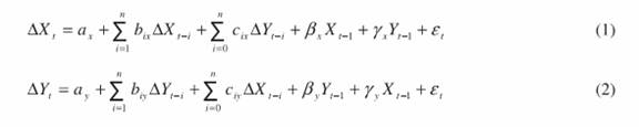
This test involves investigating the existence of a long-run
relationship among the variables using an unrestricted error-correction
model (UECM). In the case of two variables, the UECM would take the
following form:
 |
 |
The F-test has a non-standard distribution which depends upon:
(i) whether variables included in the ARDL model are I(1) or I(0); (ii)
whether the ARDL model contains an intercept and/or a trend. There are critical bound values of both the statistics set by the properties of
the regressors into purely I(1) or I(0), which are provided in Pesaran,
Shin and Smith (2001) for large sample size. The critical bound values
for F-test in the case of small sample size are estimated in Narayan
(2005). If the absolute value of the estimated F-statistics: (i) lie in
between the critical bounds set by I(1) and I(0), cointegration between
the variables is inconclusive; (ii) in absolute value lower than set by
I(0), cointegration is rejected; and iii) in absolute value higher than set
by I(1), cointegration is accepted.
For the equation which shows cointegrating relationship, the
conditional long-run relationship is estimated by the reduced form
solution of the following ARDL equations. If ‘X’ is the explained
variable the specification takes the form:
The ECT term in (7) is the error obtained from the long-run
relationship in (6).
The error correction model described by (7) can be used to
generate dynamic forecast of the explained variable based on the past
and current values of the independent variables. The accurateness of
the dynamic forecast could indicate the robustness of the estimated
model.
Section V
Data and Empirical Results
We cover the time period 1953 to 2009. The relevant data on
price (wholesale price index) and reserve money are obtained from
Monetary Statistics and Handbook of Statistics on Indian Economy,
RBI. Data on Central Government fiscal deficit from 1971 onwards
are obtained from Handbook of Statistics on Indian Economy, while that for the earlier period was taken from Pattnaik et al (1999). Two
time periods were considered, mainly with the purpose of generating
dynamic forecast and checking the robustness of the model. The first
time period is from 1953 to 2005, which excludes the post-FRBM
period when direct lending to Government by the RBI was discontinued
under the FRBM Act.
Unit Root Tests
To gauge the appropriateness of the ARDL cointegration analysis,
two unit root tests viz., ADF test and PP test were conducted for the two
sample periods. It was found that there are contradictions in the unit
root properties based on the alternative tests for the price variable and
between the two sample periods on government deficit. On the other
hand, seigniorage is indicated to be a stationary series by both the tests
and for both the sample periods. The overall picture that emerged was
that the three variables considered are not necessarily integrated of the
same order (Table 1). In view of this, we used bounds tests, which are
valid when variables are integrated of different order (Pesharan, Shin
and Smith, 2001).
Bounds Tests
Bounds test results are extremely sensitive to the presence of
serial correlation and the lag length selected. In order to remove the possible presence of serial correlations, dummies were included to
remove outliers. With price as the explained variable, the outliers
were found in 1974 and 1975 coinciding with the after affects of oil
price shock of 1973. Fiscal deficit outliers were found in 1955 and
2009, coinciding with the initiation of the Second Five Year Plan and
the recent fiscal stimulus measures following economic slowdown
due to the global financial crisis, respectively. The outliers with
respect to seigniorage were found during the years of 1975, 1976 and
1977, which were the years of extreme volatility in prices and money
growth. Given the use of annual data, the maximum lag length was
set at 2 and the appropriate lag length was selected based on SBC
criterion.1 This was considered appropriate since the sample size is
small (in the statistical sense) and therefore including too many lags
may lead to loss of explanatory power.
Table 1 : Unit Root Tests |
Variable (X) |
ADF |
PP |
X |
ΔX |
X |
ΔX |
1953 to 2005 |
|
|
|
|
LogP |
-3.21(t) |
-5.20* |
-4.94(t)* |
-6.22* |
LogS |
-5.59(t)* |
-8.93* |
5.60(t)* |
-24.4* |
LogD |
-3.10(t) |
-6.96* |
-3.16(t) |
-6.98* |
1953 to 2009 |
|
|
|
|
LogP |
-2.93(t) |
-6.43* |
-4.36(t)* |
-6.44* |
LogS |
-5.50(t)* |
-9.09* |
5.53(t)* |
-24.6* |
LogD |
-3.58(t)** |
-6.82* |
-3.63(t)** |
-6.69* |
Note: * and ** denote statistical significance at 1% an d 5% levels, respectively, ‘t’
in parentheses denote that the tests included a trend along with the constant. |
The bounds test results among the variables during both the sample
periods reported in table-2 reveal the following:
(i) Between price and seigniorage, the F-statistics are above the
95% critical bound values (9.74 and 7.18 for the two sample
periods) and significant at 99% critical level only when price
is explained by seigniorage. The F-statistics for the reverse
relationships (3.13 and 2.67) are statistically insignificant. In
other words, there exists a long-run cointegrating relationship
between price level in the economy and government resorting to
seignorage to finance its deficits, but with the former only being
caused by the latter;
(ii) Between price and government deficit, the F-statistics for the two
sample periods are 6.17 and 7.96 and statistically significant only
when price is explained by government deficit. In the case of the
reverse relationship, the F-statistics are 3.34 and 2.27 and are lower
than 95% critical bound values and hence not significant. Thus, in
the long-run, government deficit has an impact on price level in the
economy, but the reverse impact is insignificant;
(iii) Seigniorage is also explained by government deficit with
F-statistics of 8.14 and 5.32 for the two sample periods, but the reverse relationships are not statistically significant, given the
corresponding F-statistics of 0.39 and 0.48. The implication is
that government resorts to seigniorage to finance its deficit in the
long-run, but there is no significant reverse impact.
(iv) When all the three variables are combined, only price is explained
by seigniorage and government deficit with F-statistics of 6.42 and
5.83 for the two sample periods. None of the reverse relationships
are statistically significant. The respective F-statistics for the two
sample periods are 2.51 and 1.85 with government deficit as the
explained variable and 0.83 and 0.56 with seigniorage as the
explained variable. In other words, ceteris paribus, price level in
the economy in India, in the long-run, is significantly influenced
either directly by deficit itself or through the creation of money
via deficit financing, or a combination of both. In other words,
Inflation is indicated to be explained by government deficit
either directly or through seigniorage indirectly or through a
combination of both the factors. Further, the results that there
is only one cointegrating relationship between the variables in
all the alternative combinations clearly indicates that the ARDL
approach to cointegration can be used for estimation of the longrun
relationships and the short-run dynamics.2
Long-run Coefficients
In estimating the long-run Coefficients a trend component was
included in the price equations as a proxy to capture the impact
of other macroeconomic variables on price. The results presented
in table-3 reveal some interesting features. While the signs of the
Coefficients are as expected a priori in all the equations, some of them
are not statistically significant. specifically, the Coefficients of fiscal
deficit in the price equations are insignificant in the shorter sample
period (column 2 and 4), but turn significant in the full sample period
(column 6 and 8). Conversely, the Coefficients of seiniorage which
are significant in the shorter sample period (column 1 and 4) turn
insignificant in the full sample period, particularly with the inclusion
of fiscal deficit as the other explanatory variable (column 5 and 8).
Table 2 : Bounds test for Cointegration |
Functional Relationship |
1952-2005 |
1952-2009 |
F-Statistics |
95% critical Values |
Dummy variables |
F-Statistics |
95% critical Values |
Dummy variables |
Bivariates |
Fp(P/S) |
9.74* |
4.44 |
1974 & 1975 |
7.18* |
4.393 |
1974 & 1975 |
Fs(S/P) |
3.13 |
4.44 |
|
2.67 |
4.393 |
|
Fp (P/D) |
6.71* |
4.44 |
1974 & 1975 |
7.96* |
4.393 |
1974 & 1975 |
Fd (D/P) |
3.34 |
4.44 |
1955 |
2.27 |
4.393 |
1955 & 2009 |
Fs(S/D) |
8.14* |
4.44 |
1975, 1976 & 1977 |
5.32** |
4.393 |
1975, 1976 & 1977 |
Fd(D/S) |
0.39 |
4.44 |
|
0.48 |
4.393 |
2009 |
Trivariates |
Fp(P/S,D) |
6.42* |
4.178 |
1974 & 1975 |
5.83* |
4.10 |
1974 & 1975 |
Fd(D/S,P) |
2.51 |
4.178 |
|
1.85 |
4.10 |
2009 |
Fs(S/D,P) |
0.83 |
4.178 |
1959 & 1997 |
0.56 |
4.10 |
1959 & 1997 |
Note: * and ** denote statistical significance at 99% and 95% critical levels,
respectively. The critical bound values for F-statistics are from Narayan (2005). |
This could indicate that till the ban on direct government borrowing
from the RBI, the Inflationary impact of fiscal deficit worked primarily
through money creation and overshadowed the direct impact, if any.
However, in recent years, with limited scope for direct monetisation,
the Inflationary impact of fiscal deficit is generated more directly
perhaps via the channel of increase in aggregate demand.
Individually, one percent increases in seigniorage leads to about
one-third of a percent increase in the price level in both sample periods,
though the level of statistical significance declines (column 1 and 5).
With regard to fiscal deficit, one per cent increase in it leads to about one-fifth to one-quarter of a per cent increase in the price level, which
though is statistically significant only for the full sample period (column
2 and 6).
Table 3 : Long-run Coefficients |
|
1954-2005 |
1954-2009 |
(1) |
(2) |
(3) |
(4) |
(5) |
(6) |
(7) |
(8) |
LogP |
LogP |
LogS |
LogP |
LogP |
LogP |
LogS |
LogP |
Constant |
4.50 |
3.30 |
-3.01 |
3.75 |
4.53 |
3.0 |
-3.18 |
3.23 |
| |
(21.6)* |
(5.4)* |
(-12.8)* |
(6.4)* |
(17.6)* |
(5.1)* |
(-10.7)* |
(5.3)* |
LogS |
0.31 |
|
|
0.23 |
0.32 |
|
|
0.2 |
| |
(2.1)** |
|
|
(1.8)*** |
(1.7)*** |
|
|
(1.3) |
LogD |
|
0.19 |
0.483 |
0.13 |
|
0.25 |
0.51 |
0.24 |
| |
|
(1.5) |
(19.3)* |
(1.2) |
|
(2.1)** |
(16.6)* |
(2.1)** |
Trend |
0.06 |
0.05 |
|
0.05 |
0.05 |
0.04 |
|
|
| |
(6.1)* |
(3.3)* |
|
(3.4)* |
(4.0)* |
(2.9)* |
|
|
DumP |
0.71 |
0.79 |
|
0.67 |
|
0.90 |
|
0.93 |
| |
(0.71)** |
(2.6)* |
|
(2.5)** |
|
(2.64)** |
|
(2.2)* |
DumS1 |
|
|
-.97 |
|
|
|
-1.25 |
|
| |
|
|
(-3.2)* |
|
|
|
(-2.85)* |
|
Note: *, ** and *** denote statistical significance at 1%, 5% and 10% levels, respectively.
Dummy as indicated in the bounds test. |
The above estimated elasticities, however, ignore the interaction
between seigniorage and government deficit. It is seen from column
(3) and (7) that to finance one percent of fiscal deficit in the long-run,
seigniorage increased by about 0.48 to 0.51 percent, with other things
remaining the same.
Combining both government deficit and seigniorage,one percent
increase in seigniorage was found to cause Inflation by about onefi
fth of a percent in both the sample periods, but is not statistically
significant for the full period. With regard to one per cent increase
in government deficit, the impact which was small (0.13) and not
statistically significant in the shorter sample period, increased in the
full sample period to a statistically significant level of about a quarter
of a percent increase in the price level. It may, thus, be interpreted
that, in the more recent years, the direct long-run Inflationary impact of seigniroage has declined while that of government deficit through
aggregate demand channel has increased. However, the long-run
impact of government deficit on seigniorage revenue appears to have
not declined.
Short-run Dynamics
The short-run dynamics presented in Table-4 reveal that all the
equations are stable i.e., they converge to the long-run equilibrium
as indicated by the negative sign of the error correction term. The
explanatory powers are reasonable and the problem of serial correlation
is within the tolerable level in general. There, however, seems to be
some decline in the explanatory power after the inclusion of more
recent periods.
The Inflationary impact of seigniorage in the short-run is neglisible,
irrespective of whether it is considered alone or taken together with
government deficit in the model in both the sample periods (columns
1, 4, 5 and 8). The speed of convergence following a shock is also very
slow, about 16 to 17 percent in a single year when considered alone and
about 16 to 20 percent when deficit is also included.
Government deficit, on the other hand, has a positive impact on
Inflation even in the short-run for the full sample period indicating that
the direct Inflationary impact of government deficit could have become
more prominent in the more recent years.
With regard to the impact of government deficit on seigniorage,
there is a strong positive impact even in the short-run. The impact was
larger in the shorter sample period and the speed of convergence was
also higher with about 92 per cent of the divergence from the long-run
equilibrium following a shock being corrected in a single time period.
Both the short-run impact and speed of convergence decline in the full
sample period, indicating that government may have switched over
to alternative source of financing its deficit in the short-run given the
restriction on direct borrowing from the RBI since the beginning of
fiscal 2006.
Table 4 : Short-run Dynamics |
|
1954-2005 |
1954-2009 |
(1) |
(2) |
(3) |
(4) |
(5) |
(6) |
(7) |
(8) |
ΔLogP |
ΔLogP |
ΔLogS |
ΔLogP |
ΔLogP |
ΔLogP |
ΔLogS |
ΔLogP |
Constant |
0.79 |
0.62 |
-2.78 |
0.75 |
0.73 |
0.52 |
-2.38 |
0.51 |
| |
(3.1)* |
(2.7)* |
(-5.3)* |
(3.1)* |
(2.8)* |
(2.5)** |
(-4.26)* |
(2.2)** |
ΔLogP-1 |
|
|
|
|
0.33 |
|
|
|
| |
|
|
|
|
(2.4)** |
|
|
|
ΔLogS |
0.00 |
|
0.29 |
-0.00 |
-0.01 |
|
0.24 |
-0.00 |
| |
(0.01) |
|
(2.6)** |
(-0.2) |
(0.61) |
|
(1.96)*** |
(-0.6) |
ΔLogD |
|
0.04 |
0.45 |
0.03 |
|
0.04 |
0.38 |
0.04 |
| |
|
(1.5) |
(5.9)* |
(1.1) |
|
(2.2)** |
(4.8)* |
(1.9)*** |
Trend |
0.01 |
0.01 |
|
0.01 |
0.01 |
0.01 |
|
0.00 |
| |
(2.0)** |
(2.2)** |
|
(1.9)*** |
(1.6) |
(1.9)*** |
|
(1.1) |
DumP |
0.12 |
0.15 |
|
0.13 |
|
0.16 |
|
0.15 |
| |
(4.6)* |
(4.5)* |
|
(4.7)* |
|
(5.0)* |
|
(5.2)* |
DumS1 |
|
|
-0.90 |
|
|
|
-0.94 |
|
| |
|
|
(-4.0)* |
|
|
|
(-3.8)* |
|
ECM(-1) |
-0.17 |
-0.19 |
-0.92 |
-0.20 |
-0.16 |
-0.127 |
-0.75 |
-0.16 |
| |
(-2.76)* |
(-3.4)* |
(-4.93)* |
(-2.97)** |
(-2.43)* |
(-3.27)* |
(-5.17)* |
(-2.42)** |
R-bar Square |
0.52 |
0.40 |
0.57 |
0.52 |
0.27 |
0.40 |
0.46 |
0.47 |
DW-Statistics |
1.75 |
1.65 |
1.88 |
1.73 |
2.02 |
1.64 |
1.82 |
1.64 |
Note : *, ** and *** denote statistical significance at 1%, 5% and 10% levels,
respectively. Dummy as indicated in the bounds test. |
As mentioned above, dynamic forecasts of Inflation for the period
2006 to 2009 were generated from the models estimated for the period
1953 to 2005 and then compared with the actual change. The forecast
results are presented in Table-5. It could be seen that the direction
of actual Inflation are correctly predicted irrespective of whether
seigniorage and government deficit are combined or considered
individually. However, the Inflation rates in each of the four years
are over-predicted The root mean square errors of predictions for the
forecast period are also marginally higher than for the estimation period,
except when government deficit is considered as the only explanatory
variable. However, root mean square errors are about or less than 5.0
per cent, indicating that the forecast performance may be reasonable.
Table 5 : Dynamic Forecasts for 2006 to 2009 |
(in per cent) |
|
Change in P due to change in S and D |
Change in P due to change in S |
Change in P due to change in D |
|
Actual |
Predicted |
Actual |
Predicted |
Actual |
Predicted |
2006 |
4.28 |
8.8 |
4.28 |
9.67 |
4.28 |
8.1 |
2007 |
5.28 |
8.7 |
5.28 |
9.97 |
5.28 |
7.5 |
2008 |
4.65 |
9.4 |
4.65 |
11.2 |
4.65 |
6.7 |
2009 |
8.01 |
13.0 |
8.01 |
12.6 |
8.01 |
9.7 |
Root mean square |
Estimation Period |
Forecast period |
Estimation Period |
Forecast period |
Estimation Period |
Forecast period |
3.3 |
4.4 |
3.3 |
5.3 |
3.9 |
2.6 |
Section VI
Concluding Observations
The fiscal response in India to the severe contagion from the global
crisis was conditioned by the need to minimize the adverse impact on
the domestic economy. In the process, however, India’s fiscal deficit
expanded again to the pre-FRBM level. Given India’s past experience,
in terms of fiscal consolidation resulting only over a number of years,
downward inflexibility of the post-crisis high fiscal deficit level could
emerge as a potential source of risk to India’s future path of Inflation.
During 2008-10, when the fiscal stimulus led to increase in the
fiscal deficit level, India’s Inflation environment remained highly
volatile, reaching a peak in 2008-09 under the influence of the global
oil and commodity prices shock, and coming under pressure again in
2009-10 from another supply shock, but from within the country, in the
form of significant increase in food prices resulting from the deficient
monsoon. In this Inflation process over these two years, however,
fiscal deficit did not have much of a contributing role, since: (a) the
overall private demand remained depressed, and fiscal expansion only
aimed at partially offsetting the impact of deceleration in the growth
of private consumption and investment demand on economic growth,
(b) large borrowing programme of the Government did not lead to
high money growth, since the growth in demand for credit from the
private sector exhibited significant deceleration, and (c) certain fiscal
measures like cuts in indirect tax rates in fact helped in lowering the
prices of specific goods and services to some extent. Thus, the usual two channels through which fiscal deficit could cause Inflation - i.e. by
exerting pressure on aggregate demand in relation to potential output
and by leading to excessive expansion in money growth - were almost
absent. As demand for credit from the private sector has revived, and if
capital inflows remain strong on a sustained basis, the usual downward
inflexibility in fiscal deficit and its implications for the future Inflation
path will start to emerge over time.
In this context, this paper examined the empirical relationship
between fiscal deficit and Inflation over the pre-FRBM period 1953-
2005 as well as the full sample period of 1953-2009. The direct impact of
fiscal deficit through primary expansion in reserve money was studied by
using a concept of ‘seigniorage’, proxied by the annual change in reserve
money deflated by WPI Inflation.Net RBI credit to the government and
RBI’s increase in net foreign assets are the two key determinants of
growth in reserve money on the sources side, and hence, only part of
the increase in reserve money could be ascribed to the fiscal stance at
any point of time. The overall impact of the fiscal deficit on Inflation, in
turn, could operate through both increases in aggregate demand as well
as associated growth in broad money. In both direct as well as overall
analysis, thus, the role of money in Inflation becomes obvious, but that
process could be significantly conditioned by the fiscal stance.
Bounds test results presented in the study suggest that: (a) there
is a cointgrating relationship between the price level and seigniorage
financing of deficit; (b) fiscal deficit and price level also exhibit a similar
relationship, and in both cases the price level appears to be determined
by seigniorage or fiscal deficit, not the other way round; (c) the role
of seigniorage in the Inflation process may be declining over time,
particularly in recent years, even though the impact of fiscal deficit on
Inflation through aggregate demand channel might have increased; (d)
one percentage point increase in the level of fiscal deficit is estimated
to cause as much as a quarter of a percentage point increase in WPI;
and (e) as per the analysis of short term dynamics through which fiscal
deficit may get transmitted to Inflation, fiscal deficit appears to have
a positive impact on Inflation even in the short-run, though modest.
These empirical findings suggest that while the fiscal stance in India was appropriate in the context of the economic slowdown that followed
in response to the global crisis, it may have medium-term potential
ramifications for the Inflationary situation. This possibility, in turn,
highlights the significance of return to fiscal consolidation path at the
earliest, with an emphasis on the quality of fiscal adjustment, driven
by rationalisation of expenditure rather than revenue buoyancy from
stronger growth. Build up of adequate fiscal space is important not only
for ensuring stability to the high growth objective but also for enhancing
the ability to deal with such Inflationary pressures that may originate
from temporary supply shocks, as experienced in recent few years.
___________________________________________________________
* Shri Jeevan Kumar Khundrakapam and Shri Sitikantha Pattanaik are Directors in
Monetary Policy Department and Department of Economic and Policy Research,
respectively. The earlier version of the paper was presented in the 12th Conference
on Money & Finance organised by IGIDR, Mumbai during March 11-12, 2010.
The authors are grateful to the anonymous referee for useful comments. The paper
reflects the personal views of the authors.
Notes :
1 It was, however, found that increasing the maximum lag length to 3 or 4
hardly affected the results.
2 As mentioned above, for Bounds test to be valid, the long-run relationship
between the variables should be only in one direction.
References :
Aghevli, B.B., and Khan, M. (1978), “Government deficits and the Inflationary
Process in Developing Countries,” IMF Staff Papers, 25, 383-416.
Alesina, Alberto and Drazen, Allan (1991), “Why are Stabilisations Delayed?”,
American Economic Review, Vol. 81, 1170-1188.
Ashra, S., Chattopadhyay, S., and Chaudhuri, K. (2004), “deficit, Money and
Price – the Indian Experience”, Journal of policy Modeling, 26, 289-99.
Calvo, Guillermo and Vegh, Carlos (1999), “Inflation Stabilisation and BOP
Crisis in Developing Countries,” in John Taylor and Michael Woodford (Ed).,
Handbook of Macroeconomics, Volume C, North Holland.
Catao Luis and Marco Terrones (2001), “Fiscal deficits and Inflation: A New
Look at the Emerging Market Evidence”, IMF Working Paper WP/01/74.
Cecchetti, Stephen G, M. S. Mohanty and Fabrizio Zampolli (2010), “The
Future of Public Debt: Prospects and Implications”, BIS Working Papers No.
300, March.
Fischer Stanely and William Easterly (1990), “The Economics of the
Government Budget Constraint”, World Bank Research Observer, Vol. 5(2),
127-142.
Cochrane, John H. (2009), “Fiscal Stimulus, Fiscal Inflation, or Fiscal
Fallacies?”, University of Chicago Booth School of Business, February 27..
Davig, Troy and Erie M. Leeper (2009), “Monetary-Fiscal Policy Interactions
and Fiscal Stimulus”, NBER Working Paper Series 15133, July.
IMF (2009), “ The State of Public Finances Cross-Country Fiscal Monitor”,
IMF Staff Position Note (SPN/09/25), November.
Jadhav, N. (1994). Monetary Economics for India. Delhi: Macmillan India
Limited.
Khundrakpam J.K. and Rajan Goyal (2009), “Is the Government deficit in
India Still Relevant for Stabilisation?,” RBI Occasional Papers, Vol.29 (3),
Winter 2008.
Narayan, P.K. (2005), “The Saving and Investment Nexus for China: Evidence
from Co-integrating Tests”, Applied Economics, 35, 1979-1990.
Pattnaik, R.K., Pillai, S.M., and Das, S. (1999), “Budget deficit in India: A
Primer on Measurement”, RBI Staff Studies, Reserve Bank of India.
Pesaran, M. H., Shin, Y. and Smith, R.J. (2001), “Bound Testing Approaches
to the Analysis of Level Relationships”, Journal of Applied Econometrics, 16,
289-326.
Rangarajan, C., and Mohanty M.S. (1998), “Fiscal deficit, External Balance
and Monetary Growth”, Reserve Bank of India Occasional Papers, 18, 635-
653.
Reserve Bank of India (2006), Handbook of Monetary Statistics of India.
Reserve Bank of India (2009), Handbook of Statistics of the Indian economy,
2008-09.
Sarma , Y.S.R. (1982), “Government deficits, Money Supply and Inflation in
India”, Reserve Bank of India Occasional Papers. Mumbai, India.
Sargent, Thomas J. and Neil Wallace (1981), “Some Unpleasant Monetarist
Arithmetic”, Federal Reserve Bank of Minneapolis Quarterly Review, Vol.
5(3), 1-17.
Vinals, Jose and Paolo Mauro (2010), “A Strategy for Renormalising Fiscal
and Monetary Policies in Advanced Economies”, KDI/IMF Workshop, Seoul
Korea, February 25, 2010.
Woodford, Michael (2001), “Fiscal Requirements for Price Stability”, National
Bureau of Economic Research, Working Paper, 8072. |