Press Release

RBI Working Paper Series No. 07
Debt Sustainability at the State Level in India
^@Balbir Kaur, Atri Mukherjee, Neeraj Kumar and Anand Prakash Ekka

Abstract

^*The debt position of the state governments in India, which deteriorated sharply between 1997-98 and 2003-04, has witnessed significant improvement since 2004-05, reflecting the impact of both favourable macroeconomic conditions and policy efforts by the Central and state governments. The debt sustainability analysis carried out in the paper, based on empirical estimation of inter-temporal budget constraint and fiscal policy response function in a panel data framework, covering 20 Indian states for the period 1980-81 to 2012-13, indicates that the debt position at the state level is sustainable in the long run. Disaggregated level analysis, however, reveals that despite an overall improvement in debt position of the Indian states, some of the states continue to show signs of fiscal stress and increasing debt burden. The recent slowdown in growth momentum, which is likely to affect the revenue raising capacity of the state governments, may lead to further deterioration in debt position of these states. Contingent liabilities, primarily in the form of issuance of guarantees by the state governments, remain another area of concern. The strong presence of contingent liabilities calls for a holistic assessment of debt position of states by reckoning their off-budget fiscal position including the impact of operations of state public sector enterprises.

JEL Classification: H62, H63, H70

Key Words: gross fiscal deficit, public debt, state governments

I. Introduction

In line with an overall decentralising trend, the sub-national governments worldwide have been entrusted with increasing responsibilities towards delivery of public goods and services and public investment. As the concomitant expenditure requirements generally fall short of own revenue receipts and inter-governmental transfers from the national authorities, the sub-national governments have to depend on borrowed resources to meet their expenditure commitments. However, it is important to analyse whether the dependence on borrowed resources is in line with the repayment capacity of the sub-national governments. It is in this context that the assessment relating to sustainability of public debt at the sub-national level assumes significance.

In India, the state governments while playing an important role in discharging various functions assigned to them under the Constitution, often resort to borrowings to meet various development needs. It is often said that borrowing per se is not bad provided it is used for productive purposes. While this may be a desirable goal, there could be deviations for various reasons. The accumulation of debt liabilities, if left uncontrolled, may cause macroeconomic stability issues. The debt position of state governments in India, which had deteriorated sharply between 1997-98 and 2003-04, witnessed significant improvement from 2004-05 onwards. This has been attributed, among others, to the implementation of fiscal rules through the enactment of Fiscal Responsibility and Budget Management (FRBM) Acts/Fiscal Responsibility Legislations (FRLs) at the state level in early 2000s. The fiscal consolidation initiatives of the state governments were complemented by debt and interest relief measures of the Centre, and supported by a favourable macroeconomic environment following the high growth phase and a reversal of the interest rate cycle in the mid-2000s. Majority of the states have adhered to their respective debt targets set by the Thirteenth Finance Commission (FC XIII) for the period 2010-2014, though some of them continue to be under fiscal stress with unsustainable debt positions.

Despite significant improvement in the debt position of the state governments in India in the last decade, the recent growth slowdown and volatility in the financial markets have raised fresh concerns about their financial health. The slowdown in growth momentum has implications for the revenue raising capacity of the state governments, which may also constrain their debt servicing capacity, while also increasing the borrowing requirements. It is against this backdrop, the present study revisits the issue of debt sustainability at the state level in India. The debt-sustainability analysis carried out in this paper is based on three approaches: indicator-based analysis, estimation of inter-temporal budget constraint and estimation of fiscal policy response function at the state level. The analysis is mainly restricted to debt stock or outstanding liabilities of the state governments. Like other studies, the off-budget liabilities of the state governments, borrowings through special purpose vehicles (SPVs) and contingent liabilities (both explicit and implicit) have not been included in the analysis.

The paper is organised as follows. Section II defines debt sustainability. Section III presents a review of studies that have looked at this aspect in the Indian context. An overview of the need for fiscal/debt sustainability analysis at the sub-national level is provided in Section IV. Some stylised facts relating to evolution of debt of the state governments in India are presented in Section V. Section VI presents an empirical assessment of debt sustainability at the state level based on various approaches. The rationale for extending the conventional debt sustainability analysis to include off-budget fiscal position of the state governments is explained in Section VII. The concluding observations are covered in Section VIII.

II. Defining Debt Sustainability

Sustainability is a term that has been used with increasing frequency in the academic literature and multilateral policy discussions, but with different connotations under different circumstances (Balassone and Franco, 2000; Chalk and Hemming, 2000).

How one defines debt sustainability could affect the assessment regarding sustainability or otherwise of debt in an economy. In the pioneering work on debt sustainability, based on the post-Second World War US data, Domar (1944) pointed out that primary deficit path can be sustained as long as the real growth of the economy remains higher than the real interest rate. Buiter (1985) argued that sustainable policy is the one that is capable of keeping the public sector net worth to output ratio at its current level. Blanchard (1990) provided two conditions for sustainability viz., a) the ratio of debt to gross national product (GNP) should eventually converge back to its initial level, and b) the present discounted value of the ratio of primary surpluses to GNP should be equal to the current level of debt to GNP. Buiter (1985), Blanchard (1990), and Blanchard et al. (1990)¹ consider debt level as sustainable if a country’s debt to GDP ratio remains stable, and if the economy generates debt stabilising primary balance to cover that debt in future.

Typically, conventional debt sustainability analysis is an accounting based approach linked to the inter-temporal budget constraint as follows:

which states that public debt at the beginning of the period t , i.e., (B_t) equals past period debt including interest payments but adjusted for primary balance, depending on whether there is primary surplus (PS) or primary deficit (PD). The present value borrowing constraint derived from equation (1) is given below:

The transversality condition relating to the long-term solvency of public debt, when expressed in terms of GDP ratio, states that the GDP growth rate has to be lower than the interest rate so that the discounted terminal period debt ratio converges to zero ³. This implies that in case of a positive initial public debt, the sum of the cumulated discounted future public surpluses should exceed the sum of the cumulated discounted future public deficits. However, if the rate of growth of GDP is higher than the interest rate, there would be reverse stabilising effect on the ratio of debt to GDP even if a sub-national government is accumulating primary deficit⁴.

Theoretically, if the rate of growth of the economy is greater than the real rate of interest, it would allow Ponzigame in the sense that deficits can always be financed. Blanchard and Weil (1992) referred to a similar situation when they asked “The average realized real rate of return on government debt for major OECD countries over the last 30 years has been smaller than the growth rate. Does this imply that governments can play a Ponzi debt game, rolling over their debt without ever increasing taxes?”

Azizi et al. (2013) investigated the relevance of the No-Ponzi game condition and the transversality condition for 21 countries from 1961 to 2010 and found that these two conditions were simultaneously validated only for 29 per cent of the cases under examination. They argued that the government is solvent in case its debt is backed by the discounted next period surplus. For instance, in case the interest rate on public bonds is low but the expected output growth rate is large, the solvency constraint as defined above would more likely be respected, though it would be contrary to the infinite horizon transversality condition relating to relatively large real interest rate. The empirical studies reveal that transversality conditions are inconsistent with growth miracles as evident from output growth exceeding the real rate of interest for several decades in Japan between 1960 and 1990 and China between 1990 and 2010. However, it may not be possible to sustain high growth situation and/or maintain the positive growth-interest differential for all times to come; and a positive primary balance may become necessary to ensure sustainability of public debt and avoid Ponzischeme.

III. Review of Literature

In the theoretical literature, the rationale for maintaining low/sustainable level of debt is attributed, among others, to the need to ensure sustainability of fiscal policy, provide fiscal space for undertaking counter-cyclical policy or absorbing contingent liabilities without threatening debt sustainability, reduce vulnerability to crises and optimise growth by reducing the risk of crowding out of private investment, while also considering inter-generational equity and future spending needs.

In the Indian context, there are a number of studies that have looked at the issue of debt and fiscal sustainability at the state level. Rajaraman et al. (2005) examined the issue of debt sustainability at the state level covering the time period 1992-2003. The study drew attention to a sharp rise in debt of major states during the quinquennium 1997-02 over the average for the quinquennium 1992-97. As the interest rate on state debt exceeded the nominal growth rate of GSDP during 1997-2002, it highlighted the need for fiscal correction to stabilise debt as a per cent of GSDP. The study also identified states in need of expenditure compression and improvement in own revenue collection efforts, and suggested several institutional reforms, such as, establishment of consolidated sinking fund, guarantee redemption fund and introduction of a cap on guarantees and fiscal responsibility legislations (FRLs).

Nayak and Rath (2009) studied debt sustainability for Special Category States covering the period 1991-2009. Using the Domar’s sustainability condition⁵, they found that the sustainability condition was achieved in all the states except Arunachal Pradesh. However, the solvency condition was satisfied only in the case of Assam.

Misra and Khundrakpam (2009) pointed out that the primary revenue balance, on average, at state level had not been adequate enough to meet interest payments. Using the Present Value of Budget Constraint (PVBC) approach, the liabilities of the state governments during 1991-92 to 2007-08 were found to be unsustainable.

Dholakia et al. (2004) assessed debt sustainability of states in relation to a uniform target of debt to GSDP ratio of 35 per cent and the ratio of debt to state’s own revenue during the period 1988-89 to 2003-04; a potential declining trend in the latter was interpreted as an indicator of sustainability. Based on the first indicator, it was observed that there was a debt problem of credible magnitude only in about half of the 25 states covered in the study. However, their analysis, based on the second measure, pointed out that there could be a serious problem of intolerable debt in the long-run equilibrium in two states where the interest payments to revenue receipts ratio was above the tolerable limit of 20 per cent.

Makin and Arora (2012) examined fiscal sustainability at the state level covering the time period 1990-91 to 2009-10. They estimated primary balances required to (i) stabilise public debt levels and (ii) achieve targeted debt to GSDP ratios for the individual states. The empirical exercise showed that majority of the states have stabilised public debt levels as a proportion of GSDP, reducing the risk of public debt growing without bound above present levels given the current nominal effective interest rates and the strong growth performance at the state level. However, the slowdown in economic growth could expose many Indian states to considerable fiscal risk. States, therefore, need to focus on the primary budget balance to lower their public debt to income levels.

Dutta et al. (2010) in their study on fiscal and debt sustainability of Assam, covering the period 1991-2010, pointed out that a higher proportion of revenue deficit in fiscal deficit had created the problem of fiscal instability in some years during the period of study. However, the debt-GSDP ratio declined, reflecting positive ‘Domar gap’⁶ and primary surplus enjoyed by the state in some years during the period under study. Using cointegration analysis, it was found that the state could maintain fiscal sustainability during the period under consideration.

Ianchovichina et al. (2006) studied fiscal sustainability in the state of Tamil Nadu in terms of the response of key components of the state’s fiscal accounts to reforms and shocks. The results of the study, covering the period 1990-91 to 2003-04, showed that Tamil Nadu had embarked on a fiscally sustainable path with its debt projected in the ‘baseline scenario’ to decline from 28 per cent of GSDP in 2003-04 to 16 per cent by 2026-27. However, with a positive shock of one standard deviation to real interest rate above its historical average, and a negative shock of one standard deviation below the historical avarages of GSDP and primary balances, the debt of the state was projected to grow to around 34.6 per cent in 2026-27, which was twice the ‘baseline ratio’. The fiscal adjustment path was considered to be ambitious by historical standards and politically challenging, but it left fiscal space for increases in infrastructure investment which may be achieved without threatening fiscal sustainability. It was, therefore, suggested that the state should run primary surpluses between 2 and 3 per cent of GSDP to avoid further increases in debt-GSDP ratio assuming no improvement in growth and no decline in real interest rate.

Dasgupta et al. (2012) examined debt sustainability of six of the Indian state governments during the period 2003-12. Of the six states, three states financed their revenue expenditure largely through tax receipts while the other three did not. In the process, the states in the first group could use their borrowings to finance capital expenditure that would add to their future productive capacity. Nevertheless, there was a reduction in debt-GSDP ratios of all the states during 2003-12, reflecting their adherence to Fiscal Responsibility and Budget Management Acts.

Overall, the empirical studies on debt sustainability at the state level in India indicate a mixed picture. While some of the studies point out that the debt position of states is unsustainable, others have drawn attention to the declining debt-GSDP ratios at the state level and attributed the improvement to the strong growth performance and implementation of Fiscal rules during the 2003-2012 period. However, it is also recognised that a slowdown in growth momentum could pose risk to the achievement of envisaged gross fiscal deficit and debt-GSDP targets under the medium-term scenario.

IV. Need for Assessment of Debt Sustainability at the State level

Globally, sub-national governments (SNGs) have assumed importance in the wake of their increasing role in provision of various essential services, while also catering to urban infrastructure requirements. In this process, their resource base has also expanded with growing dependence on borrowed funds. However, the borrowing limits of SNGs are by and large regulated by the upper tiers of government in countries with a federal system. Apart from the imposition of restrictions on borrowing limits, explicit co-ordination agreements between different government tiers have also been observed in several countries.

While the overall approach for assessing debt sustainability at the state level is similar to that at the Central government level, there are a few notable differences in respect of debt sustainability analysis at the state level. The state governments cannot benefit from seigniorage revenues which accrue to the central government. State finances are additionally affected by the Central government policies including legal mandates and existence of vertical imbalances. With defined (and limited) sources of own revenue receipts, states have to heavily rely on devolution of funds from the Centre which enhances their resource capacity and enables them to undertake expenditure on provision of various services on a sustained basis. State government borrowings require Central government’s concurrence. In terms of the inter-temporal budget constraint, a sustainable level of debt refers to the outstanding debt stock level that does not exceed present value of current and future primary surpluses. By this approach, theoretically the investors would finance debt only if it is deemed sustainable. De facto, however, credit risks on state borrowings may get compromised in case there is an implicit backing from the Central government. Similarly, spreads of the yields on state government debt over those of the Centre across states may not reflect their fiscal performance, in case the market participants factor in implicit Central government backing or offsets by market/liquidity factors. Further, with the monetary policy being determined at the national level, the state governments generally tend to be takers of the general interest rate environment. In addition, the Centre also influences state finances through the wage setting process of government employees, thereby exogeneously impacting committed expenditures of the state governments.

Against this backdrop, the starting point of the debt sustainability exercise is an examination of the issue as to whether the state governments really face hard budget constraints? Under Article 293(3)⁷ of the Indian Constitution, a state may not without the consent of the Government of India raise any loan if there is still outstanding any part of a loan which has been made to the state by the Government of India or by its predecessor Government, or in respect of which a guarantee has been given by the Government of India or by its predecessor Government. This implies that the state governments do not have unrestricted power to borrow as long as they are indebted to the Centre⁸. In addition, states are also prohibited from borrowing abroad with the exception of loans for externally aided projects intermediated by the Central government⁹.

In addition to the restrictions under Article 293 of the Constitution of India, the state governments have gone ahead with the self-imposed restrictions through the enactment of FRBM Acts/FRLs. The implementation of a rule-based fiscal discipline mechanism under these enactments has been marked by a gradual move towards sustainability of their fiscal and debt positions, with majority of the states achieving the FC XIII targets as also their self-imposed targets. However, a few states continue to face fiscal stress and their debt positions remain an area of concern. Furthermore, notwithstanding strict monitoring of overall borrowing limits and adherence to various restrictions¹⁰, the states have been able to raise additional ‘off-budget’ borrowings with guarantees through state controlled special purpose vehicles (SPVs) and/or state-owned public sector enterprises (SPSEs). It is against this backdrop that the following Section presents the evolution of debt position of state governments beginning 1980-81.

V. Evolution of State Government Debt in India: Some Stylised Facts

The fiscal position of the state governments had remained comfortable in the first three decades since independence. The state finances exhibited signs of fiscal stress since the mid-1980s. However, the debt position of states generally remained under control during the period 1980-81 to 1996-97, with an average debt-GDP ratio at 18.3 per cent and 20.8 per cent during 1981-82 to 1991-92 and 1992-93 to 1996-97, respectively. The period from 1997-98 to 2003-04 was marked by a sharp deterioration in key deficit indicators of the state governments, which was reflected in an increase of around 6 percentage points in average debt-GDP ratio to 26.9 per cent. The actual debt-GDP ratio reached a high of 31.8 per cent in end-March 2004 (Chart I.a).

In recognition of the need for fiscal discipline, the state governments, however, adopted a rule-based fiscal framework through the enactment of FRBM Acts/FRLs which also included stipulation of ceilings on total liabilities and in some cases on debt-service liabilities. Karnataka was the first state to enact its FRBM Act in September 2002, followed by Kerala (2003), Tamil Nadu (2003) and Punjab (2003). Other states also adopted these legislations to avail of the benefits under the incentive scheme recommended by the Twelfth Finance Commission (FC XII)¹¹. The adherence to these legislations was also supported by the implementation of Debt Swap Scheme (DSS) from 2002-03 to 2004-05 and Debt Consolidation and Relief Facility (DCRF) from 2005-06 to 2009-10. These two debt restructuring schemes provided debt relief through debt consolidation, and reduced interest burden on the states. In addition, a turnaround in interest rate cycle also contributed to a gradual reduction in effective interest rates and debt servicing costs during this period. These developments were mirrored in lower debt-GDP ratio at 26.6 per cent in end-March 2008, before declining further to 21.7 per cent in end-March 2013. However, at a disaggregated level, the debt-GSDP ratio was higher than 30 per cent level in Punjab, Uttar Pradesh and West Bengal, while it exceeded 25 per cent level in Goa and Kerala (Table 1). Odisha recorded a remarkable improvement in its debt-GSDP ratio during the period 2004-05 to 2012-13.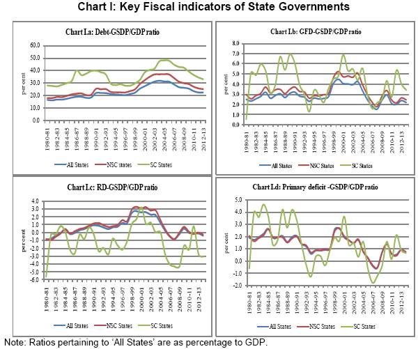

NSC = Non-special category states, viz., Andhra Pradesh, Bihar, Chhattisgarh, Goa, Gujarat, Haryana, Jharkhand, Karnataka, Kerala, Madhya Pradesh, Maharashtra, Odisha, Punjab, Rajasthan, Tamil Nadu, Uttar Pradesh and West Bengal

SC = Special category states, viz., Arunachal Pradesh, Assam, Himachal Pradesh, Jammu & Kashmir, Manipur, Meghalaya, Mizoram, Nagaland, Sikkim, Tripura and Uttarakhand.

VI. Assessment of Debt Sustainability at the State Level

In the empirical literature, there are primarily two approaches to fiscal (debt) sustainability. The first approach looks at various indicators of sustainability of fiscal policy (Miller 1983, Buiter 1985, 1987, Blanchard 1990, Buiter et al. 1993) while the second approach involves empirical evaluation or tests of government solvency (Hamilton and Glavin 1986, Trehan and Walsh 1988, Bohn 1998). The empirical testing techniques include determination of sustainable level of public debt based on a partial equilibrium framework, a model-based approach and signal approach to fiscal sustainability. Marini and Piergallini (2007), however, suggest an integration of the results from these two approaches so as to provide additional information on the issue of government solvency. While indicators are said to be forward looking, empirical tests are considered backward looking as they are based on historical data. It is the stability of the parameters of the primary surplus equation that determines the use of results from indicators or from tests in the assessment of the sustainability of public debt. It is held that “without a systematic break in policy, the predictions of tests are more reliable since the results of indicators are likely to reflect cyclical factors”. We have used both indicator-based approach and empirical testing techniques for an assessment of debt sustainability at the state level in India.

VI.1:Indicator-based Assessment

Traditionally, debt sustainability has been assessed in terms of indicator analysis. The assessment is generally done in terms of credit worthiness indicators (nominal debt stock/own current revenue ratio; present value of debt service/own current revenue ratio) and liquidity indicators (debt service/current revenue ratio and interest payment/current revenue ratio). These indicators broadly enable an assessment of the ability of the government to service its interest payments and repay its debt as and when they become due through current and regular sources of revenues excluding temporary or incidental revenues as grants or capital revenue resulting from sale of assets. Alternatively, debt and debt service indicators are monitored to assess relationship of existing debt to different types of expenditures or as ratios to various fiscal balances so as to gauge sustainability of both debt and fiscal situation.

Improvement in fiscal conditions creates fiscal space, and enhances debt repayment capacity, while worsening of fiscal conditions entails higher borrowings, adding to the debt burden. Improvement in debt-servicing conditions may also be policy-induced like the Debt Swap Scheme that was operational in India during 2002-03 to 2004-05, enabling states to pre-pay high cost loans contracted from the Central government through low coupon bearing small savings and current loans available from the market and thereby reducing their debt service burden. From an analytical point of view, both trends in indicators as also characteristics of institutions matter for an assessment of debt sustainability at the state level. In addition, debt sustainability is also associated with a non-financial dimension about the capacity to plan, organise and implement policies, which may be both budget and debt-related.

A snapshot picture of fiscal position of the state governments including the major deficit indicators during the period from 1980-81 to 2012-13 is presented in Tables 2.a and 2.b.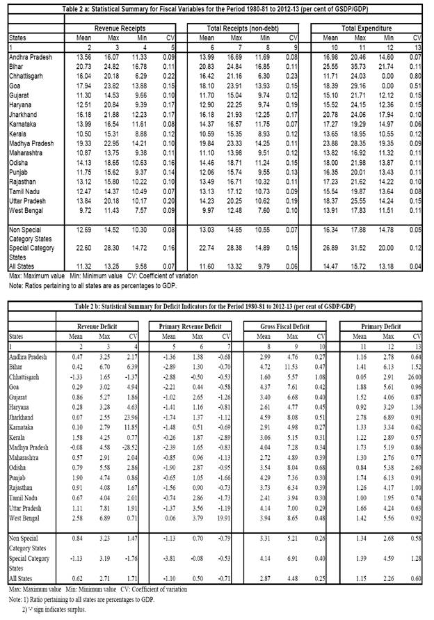

An analysis based on various indicators of debt sustainability¹² in different phases during the period from 1981-82 to 2012-13 (Table 3) reveals that the rate of growth of debt of states at the aggregate level exceeded the nominal GDP growth rate during Phase I (1981-82 to 1991-92) and Phase III (1997-98 to 2003-04). However, the real rate of interest on debt (i.e., effective interest rate¹³ adjusted for inflation) remained lower than the real output growth in all the phases except in Phase III when it was almost equal to the real output growth. The strain on state finances in Phase III was reflected in deterioration in all the indicators of sustainability, with a sharp rise noticed in debt service burden. During this phase, the Domar stability condition was also not fulfilled in a few years with real effective interest rate exceeding the real GDP growth rate.

Primary balance ratio was negative in all the phases while primary revenue balance ratio deteriorated sharply in Phase III, before showing some improvement in Phase IV. The improvement in various debt sustainability indicators in Phase IV was driven by fiscal correction measures undertaken by the state governments, debt restructuring initiatives of the Central government based on the FC XII’s recommendations and favourable interest rate environment. Interest payments, which had crossed one-fifth of revenue receipts (considered as a tolerable ratio of interest burden, Dholakia et al. 2004¹⁴) during Phase III declined to around 16 per cent in Phase IV (Annex II). However, the debt repayment capacity and interest burden indicators in Phase IV lagged behind their respective performance levels achieved in Phase I.

The positive gap between the rate of growth of GDP and effective interest rate in all the phases, except Phase III, turned out to be a predominant factor that influenced the movement of debt-GDP ratio during the period under review (Chart II).

A disaggregated state-wise position in respect of various debt sustainability indicators for 17 non-special category states (NSC) is presented in Table 4. It may be seen that most of the states have met two of the debt sustainability conditions during the latest period (2004-05 to 2012-13). For instance, during this period, the rate of growth of public debt is lower than the growth rate of nominal GSDP for all the states except Jharkhand. Similarly, the rate of growth of GSDP is higher than the effective interest rate in all the states. However, the third condition, i.e., the rate of growth of public debt should be lower than effective interest rate is met by only two states, viz., Bihar and Odisha.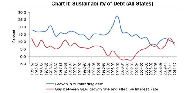

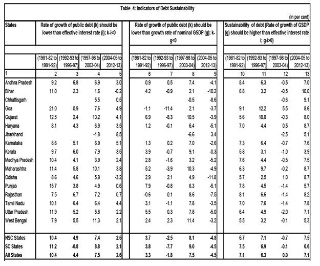In addition to the debt sustainability indicators as discussed above, it may also be appropriate to analyse debt profile linked vulnerability indicators viz., spread on state government debt, average maturity and ownership pattern of debt. These indicators provide an idea about liquidity and pricing risks associated with the level of debt and its profile. From 1988-89 onwards, the weighted average yield on state government securities has been observed to be marginally higher than that on the Central government securities. Before this period, these loans were intermediated by the Central government. The ownership pattern of state government securities indicates a pre-dominance of commercial banks, although their share in total outstanding state government securities has declined steadily from 78.5 per cent in end-March 1991 to 61.9 per cent in end-March 2000 and further to 51.1 per cent in end-March 2012. The share of insurance companies has, however, increased significantly during the same period. This is indicative of captive market for state government securities and preference of long-term investors for these securities due to higher yield vis-a-vis that on the Central government securities. The state-specific fiscal performance related risk factors are presumably not being factored in by the investors¹⁵.

VI.II:Econometric Framework for Assessing Debt Sustainability at State Level

The fiscal/debt sustainability exercise, in the empirical literature, is extended beyond the simple indicator based assessment to validate whether inter-temporal government budget constraint is satisfied. This entails test of stationarity properties of the government debt stock (in level and first difference), examination of the long-term relationship between government revenues and expenditures, between primary balances and debt, and between capital expenditure and public debt (Bhatt, 2011¹⁶). While confirmation of stationarity of government debt stock (in level and first difference) indicates statistical reversion towards mean value after temporary disturbances, the presence of cointegration between government revenues and expenditures reflects their co-movements and anchoring of fiscal imbalances.

Inter-temporal Budget Constraint

In line with the empirical literature, we have made an attempt to test whether the fiscal policy stance of Indian states is sustainable, i.e., whether it satisfies the inter-temporal budget constraint. This test basically examines whether the past behaviour of state governments’ revenue, expenditure and the fiscal deficit could be continued indefinitely without prompting an adverse response from the investors who finance their borrowings.

The inter-temporal budget constraint, under the assumption that the funding of interest payments are not made from the new debt issuances (i.e., no-Ponzi scheme), imposes restrictions on the time series properties of government expenditure and revenues. This requires that government expenditure, revenue and debt stock are all stationary in the first differences. The stationarity property also restricts the extent of deviation of government expenditure from revenues over time. In case government expenditure and revenues are I (1) and co-integrated, then the error correction mechanism would push government finances towards the levels required by the inter-temporal budget constraint and ensure fiscal and debt sustainability in the long-term (Cashin and Olekalns 2000).

In this section, first the stationarity properties of the stock of government debt, government expenditure and revenues have been tested in a panel data framework, using annual data for the period 1980-81 to 2012-13 for 20 Indian states. In addition, an attempt has been made to test, whether a long-run equilibrium exists between government expenditure and revenues through panel cointegration tests.

Data

All data on state government expenditure, revenues and outstanding level of debt have been taken from the ‘Handbook of Statistics of the Indian Economy’, published by the Reserve Bank of India. The data covers the period from 1980-81 to 2012-13 for 20 Indian states. A list of the states selected for the present analysis is presented in Annex III.A. Only those states have been selected, for which data on all the relevant variables are available for the entire time period. In the case of three states, viz., Bihar, Uttar Pradesh and Madhya Pradesh, the data on respective fiscal variables from 2000-01 also include data relating to Jharkhand, Uttarakhand and Chhattisgarh, respectively. This has been done for two reasons: first, data for Jharkhand, Uttarakhand and Chhattisgarh are available only since 2000-01, i.e., the year when these states were created; second, the data for the original states of Bihar, Uttar Pradesh and Madhya Pradesh for the period prior to 2000-01 are not strictly comparable with the data for the post 2000-01 period when these states were bifurcated. The variables have been converted into real terms with logarithmic transformation.

Unit Root Analysis

The stationarity properties of expenditure, revenues and debt of the state governments are tested through panel unit root tests. Panel unit root tests are generally perceived to be more powerful than unit root test applied on a single series. This is because the information content of the individual time series gets enhanced by that contained in the cross-section data within a panel set up (Ramirez, 2006). There are different methods to carry out panel based unit root tests. While tests viz., Levin, Lin and Chu (2002) and Hadri (2000) assume that there is a common unit root process across the relevant cross sections, the tests suggested by Im, Pesaran and Shin (2003) and Maddala and Wu (1999) assume individual unit root process.

The results of panel unit root tests on relevant fiscal variables (debt, total revenue and total expenditure) are furnished in Table 5. It may be seen that the tests (Levin, Lin and Chu; Im, Pesaran and Shin; and Maddala and Wu) fail to reject the null hypothesis of a unit root for each of the variables in level form. The tests, however, reject the null of a unit root in the first difference. The results of panel unit root test using Hadri Z test statistics are also reported in Table 5. As opposed to other tests, the Hadri test assumes a null hypothesis of no unit root. The results of the Hadri test are consistent with those of the other tests as it rejects the null of no unit root for the variables in level form. Overall, the results reveal that the three variables viz., debt, total revenue and total expenditure are non-stationary but integrated of order 1, i.e., I (1).

Panel Cointegration

Since government expenditure and revenues were found to be I (1), in the next step, an attempt has been made to test, whether there exists a long-run equilibrium (steady state) between them through panel cointegration tests. Panel cointegration technique has an advantage over the cointegration tests for individual series as it allows to selectively pool information regarding common long-run relationships from across the panel while allowing the associated short-run dynamics and fixed effects to be heterogeneous across different members of the panel (Pedroni 1999).

In this section, the methodology proposed by Pedroni (1999) has been used to test whether a co-integrating relationship exists between government expenditure and revenues of the Indian states. This method employs four panel statistics and three group panel statistics to test the null hypothesis of no cointegration against the alternative hypothesis of cointegration. In the case of panel statistics, the first-order autoregressive term is assumed to be same across all the cross sections. On the other hand, in the case of group panel statistics, the parameter is allowed to vary over the cross sections. The statistics are distributed, in the limit, as standard normal variables with a left hand rejection region, with the exception of variance ratio statistic. The results of the cointegration tests are presented in Table 6.

The test results for both the panel and group statistics reveal strong evidence of panel cointegration. The estimated ‘rho’ statistic, Augmented Dickey Fuller ‘t’ statistic and the Phillips and Perron (non-parametric) ‘t’ statistic reject the null hypothesis of no cointegration at 1 per cent level for all the three models : (i) model with no deterministic intercept or trend; (ii) model with individual intercept and no deterministic trend; and (iii) model with individual intercept and individual trend. This implies that the cointegration results are not affected by different modelling assumptions. The only exception is panel variance ratio statistic in the model with individual intercept and trend.

The results of the Pedroni test are also supported by Kao residual cointegration test, which rejects the null hypothesis of no cointegration at 1 per cent level (Table 7). Thus, the overall findings of the panel cointegration tests reveal that the two series, viz., government expenditure and revenue are co-integrated indicating a long-term co-movement between them. The results suggest that the current fiscal policies in India are sustainable in the long-run.

Fiscal Policy Response Function

Bohn (1998), Adams et al. (2010) and Tiwari (2012) have looked at the response of primary surplus to variations in public debt for the purpose of assessment of fiscal policy/debt sustainability. In this approach, it is analysed whether primary surplus relative to GDP is a positive function of public debt (relative to GDP). If such is the case, rising debt ratios lead to higher primary surpluses (or reduction in primary deficit) relative to GDP that indicates a tendency towards mean reversion. We have also used this approach in the following analysis.

Model Specification

The following equation is estimated in a panel data framework with annual data from 1980-81 to 2012-13.

Here GSDP is the gross state domestic product; S is the primary balance to GSDP ratio; D is the states’ debt to GSDP ratio; GSDPGAP is the deviation of actual output from the trend; EXPGAP is the deviation of actual primary expenditure from the trend; ε is the error term. The business cycle variable GSDPGAP has been included to account for the fluctuations in revenues. The variable EXPGAP captures the impact of deviations of real primary expenditure from its long-term trend on the primary balance ratio. Here ‘β’ is the key coefficient, which measures the response of primary balance to debt. A value of this coefficient between zero and unity is consistent with a sustainable fiscal policy response to debt. A negative coefficient implies potentially destabilising response. In addition, allowance has been made in the estimations for the response of primary balance to GSDP ratio to be non-linear and vary with debt levels by introducing a square term of the debt to GSDP ratio as an additional explanatory variable.

Data

Annual data for the period 1981-82 to 2012-13 for 20 Indian states have been used for the analysis. Only those states have been selected, for which data on all the relevant variables are available for the entire time period (Annex III.A). As in the earlier case (inter-temporal budget constraint), for three of the states, viz., Bihar, Uttar Pradesh and Madhya Pradesh, the data from 2000-01 also include data relating to Jharkhand, Uttarakhand and Chhattisgarh, respectively. Outstanding liabilities of each state government have been used to represent the level of their debt. GSDPGAP for each state has been worked out by extracting the deviation in real GSDP from its trend through HP-filter. The deviation is expressed as a per cent of real GSDP. EXPGAP has been calculated in a similar manner using real primary expenditure of the state governments. The pair-wise correlation coefficients between the explanatory variables were found to be statistically insignificant, thus ruling out any multicolinearity problem.

Results

Before proceeding with the estimation, all the series were tested for stationarity. Based on panel unit root tests involving common unit root process (LLC) as well as individual unit root process (IPS), the dependent variable and the explanatory variable series were found to be stationary, i.e., I (0). The results of the panel unit root tests are furnished in Table 8.

To decide on the panel models, i.e., whether it is a fixed effect (FE) model or a random effect (RE) model, Hausman test was conducted for each of the two model specifications (linear and non-linear). The summary results of the Hausman test are furnished in Annex III.B. The results of the Hausman test for both the models indicate that there is a significant difference in the coefficients estimated by the FE and RE models. Therefore, the null hypothesis of correlated random effect is rejected and the alternative hypothesis that individual specific effect is correlated with the explanatory variables is accepted. Accordingly, fixed effect model has been chosen for estimating the two model specifications indicated above.

The models have been estimated through generalised least square technique with cross section Seemingly Unrelated regression (SUR) with a correction for first order autoregressive error term. The models are adjusted for the heteroskedasticity with White cross-section standard errors and covariance method. The empirical results from the panel regression exercise are presented in Table 9. In Model 1 (linear model), the coefficients of all the explanatory variables were found to be significant at one per cent level. Positive coefficient of D indicates that primary balance of the state governments increase in response to rising debt ratios. This implies that the primary fiscal balance in India responds in a stabilising manner to increases in debt. Positive coefficient of GSDPGAP implies that primary balance improves when GSDP is above the trend. The negative coefficient of EXPGAP, on the other hand, indicates that primary balance declines when primary expenditure is above the trend. These findings are in line with the a priori expectations.

In the non-linear equation approach (Model 2), allowance was made for the possibility that the response of the primary balance to debt is better represented in terms of a quadratic function rather than a linear response function. The results suggest that the primary balance function has an inverted ‘u’ shape, implying that the adjustment parameter first rises and then falls.

VII. Going beyond the Conventional Debt Sustainability Analysis

In the empirical literature, the focus has recently been on a more comprehensive assessment of debt sustainability in various ways. This is done using a broader coverage of debt including contingent, implicit and also off-budget liabilities. The conventional debt sustainability analysis, based on the inter-temporal budget constraint, is extended to account for fiscal and economic behaviour in response to shocks (sensitivity analysis), fiscal vulnerabilities (stress-testing exercise) and short-term refinancing risks. The interaction of key variables driving debt dynamics is also factored in debt sustainability exercises.

We have not attempted debt sustainability analysis at the state level in a dynamic environment which involves simulation and sensitivity exercises to account for the impact of shocks and deviations from the baseline assumptions relating to macroeconomic parameters on the evolution of public debt path in future to judge whether it would remain sustainable or not. However, the issuance of guarantees by the state governments has remained an area of concern.

In recognition of the fiscal risk associated with guarantees, both fresh issuances and outstanding, a ‘Group of State Finance Secretaries on the Fiscal Risk on State Government Guarantees’ (2002) had underlined the importance of according appropriate risk weights in respect of devolvement of guarantees, and making adequate budgetary provisions for honouring these guarantees in case they devolve on the states. State-wise data on explicit guarantees from 1990-91 onwards indicates that there has been a declining trend in outstanding guarantees at the aggregate level in the 2000s. This also reflects the impact of fixation of limits on annual incremental guarantees¹⁷ as ratio to GSDP or total revenue receipts under the FRBM Acts/FRLs enacted by the state governments. Notwithstanding the same, these explicit contingent liabilities in end- March 2012 have increased substantially in some states and thus pose a risk to continued fiscal/debt sustainability in the medium-term in case these liabilities materialize. The guarantee commitments of state governments in respect of state public sector enterprises (SPSEs) are, in fact, a major source of potential risk to fiscal and debt sustainability at the state level in general¹⁸ and those states in particular where SPSEs have accumulated huge losses and debt liabilities. In addition, contingent liabilities linked to public-private partnership (PPP) projects and unfunded liabilities relating to pension are other risk factors.

It is evident that a fair assessment of debt sustainability at the state level would be possible in case contingent and other implicit liabilities are also accounted for in the empirical exercise. However, this could be an area of future research provided more detailed information on these liabilities at the state level becomes available.

VIII: Conclusion

In this paper, the debt sustainability of the state governments in India was assessed through indicator-based analysis as well as empirical exercises. The indicator-based analysis revealed that while most of the debt sustainability indicators showed significant improvement during 2004-05 to 2012-13 compared to the earlier phase (1997-98 to 2003-04), debt repayment capacity and interest burden indicators lagged behind their respective performance levels achieved during 1981-82 to 1991-92.

The estimation results based on a panel data framework covering 20 Indian states for the time period 1980-81 to 2012-13 revealed that there is a co-integrating relationship between government expenditure and revenues in India, which tantamount to satisfying the inter-temporal budget constraint. Moreover, the estimated fiscal policy response function indicated that the primary fiscal balance in Indian states responds in a stabilising manner to the increase in debt. Thus, both the results indicate that the current debt situation at the state level is sustainable in the long-run.

Disaggregated level analysis, however, revealed that despite an overall improvement in debt position of the Indian states, some of the states continue to show signs of fiscal stress and increasing debt burden. Going forward, there may be downside risks in case the slowdown in growth momentum observed during the last two years persists, with its likely adverse implications for the revenue raising capacity of the state governments. The state governments will have to keep their primary expenditure under control in order to avoid their increasing dependence on borrowed funds

Vulnerability analysis based on different indicators viz., spread, average maturity and ownership pattern of state government debt, which provide an idea about liquidity and pricing risks associated with the level of debt and its profile, showed the presence of captive market for state government securities and preference of long-term investors for these securities due to their higher yield vis-a-vis that on the Central government securities. From this, it appears that the investors perceive their investment in state government securities to be credit-risk free. The state-specific fiscal performance related risk factors are presumably not being factored in by the investors.

Overall, the conventional debt sustainability analysis, as attempted in this paper, shows that debt position of states at the aggregate level is sustainable. However, this analysis has its own limitations as it focuses primarily on explicit debt liabilities. In case, the contingent and implicit liabilities were to be accounted for, the position could be different from what has been observed on the basis of explicit debt liabilities.

^@ Balbir Kaur is Adviser, Atri Mukherjee and Neeraj Kumar are Assistant Adviser and Anand Prakash Ekka is Research Officer in the Department of Economic and Policy Research, Reserve Bank of India.

^* The views expressed in the paper are those of the authors and do not necessarily reflect the views of the Reserve Bank of India. The authors are thankful to the anonymous referee for valuable comments on the paper. The authors would also like to thank Smt Deepa S. Raj and Dr. Saibal Ghosh for their valuable suggestions and comments.

¹ Blanchard et al. (1990) estimated threshold (sustainable and long-run) debt levels for advanced economies and emerging markets (EMs) at 75 per cent and 25 per cent of GDP, respectively. Using parametric method and signal approach, IMF (2011) estimated the maximum sustainable debt level for EMs at 78 per cent and 63 per cent of GDP, respectively.

² Fiscal sustainability hypothesis also assumes validity of Ricardian equivalence, i.e., trajectory of main macroeconomic variables is not affected by choice of issuance of debt and increase in taxation.

³ The derivation of the solvency condition is based on the assumption that the real interest rate after subtracting the real growth rate is positive in case an economy is dynamically efficient.

⁴ Ball et al. (1995) found that the average of interest rate minus GDP growth rate was slightly negative for the US; Mishkin (1984) found similar result for other countries.

⁵ Real growth rate should be higher than the real interest rate.

⁶ Real GSDP growth exceeded the real interest rate.

⁷ Under the provisions of Article 293, the executive power of a State extends to borrowing within the territory of India upon the scrutiny of the Consolidated Fund of the State within such limits, if any, as may from time to time be fixed by the Legislature of such State by law and to the giving of guarantees within such limits, if any, as may be so fixed.

⁸ Borrowings under small savings collections were earlier exogenously determined depending on collections under the geographical jurisdiction of the state and were outside the purview of Article 293 (3) of the Constitution.

⁹ These loans are being passed on to non-special category state governments on a ‘back-to-back’ basis under the same terms and conditions from April 1, 2005.

¹⁰ While states have an automatic entitlement to small savings collections within the jurisdiction of their respective State, depending on the sharing arrangement between the Centre and States, any shortfall/excess under this head under the extant monitoring arrangement with an overall cap on borrowings is adjusted against market borrowings.

¹¹ All the states have since enacted FRBM Acts/FRLs.

¹² These are furnished separately for non-special category and special category states in Annex I.A and I.B, respectively.

¹³ Effective interest rate represents current interest payments as a per cent of outstanding liabilities of state governments in the previous year.

¹⁴ Debt is considered tolerable if its servicing does not impose disproportionately heavy burden on the revenues of a State.
Dholakia also suggested that fiscal performance ratios should be assessed in terms of state’s own revenues and not GSDP because the latter involves an unknown margin of error.

¹⁵ McCarten (2003) points out absence of any correlation between state creditworthiness and risk premia on interest rates borne by the state governments in India, preventing the emergence of a market-based fiscal discipline regime for states. This is also corroborated by the results of a paper by Bose et al. (2011).

¹⁶ Antra Bhatt (2011) examined the long-term relationship between capital expenditure and public debt in India in a co-integrating framework during the time period 1980-2009.

¹⁷ The concept of risk-weighted guarantees is yet to be adopted by the state governments.

¹⁸ The issuance of guarantees/letters of credit to SPSEs poses a fiscal risk especially when cost recovery systems are not fully in place (Reddy 2001).

References

Adams, Charles, Benno Ferrarini and Donghyun Park (2010), “Fiscal Sustainability in Developing Asia”, ADB Economics Working Paper Series, No. 205

Azizi, Karim, Nicolas Canry, Jean-Bernard Chatelain and B. Tinel (2013), “Government Solvency, Austerity and Fiscal Consolidation in the OECD: A Keynesian Appraisal of Transversality and No Ponzi Game Conditions”, April, Cornell University Library, accessed from http://arxiv.org/abs/1304.7330

Balassone, F. and D. Franco (2000), “Assessing Fiscal Sustainability: A Review of Methods with a View to EMU”, in Banca d’Italia (2000)

Bhatt, Antra (2011), “Revisiting Indicators of Public Debt Sustainability: Capital Expenditure, Growth and Public Debt in India”, MPRA Paper No. 28289

Blanchard, O.J. (1990), “Suggestions for a New Set of Fiscal Indicators”, OECD Economics Department Working Paper N. 79

Blanchard, O., J.C. Chouraqui, R.P. Hagemann and N. Sartor (1990), “The Sustainability of Fiscal Policy: New Answers to Old Questions”, OECD Economic Studies, No. 15

Blanchard O.J. and P. Weil (1992): Dynamic Efficiency, the Riskless Rate, and Debt Ponzi Games under Uncertainty, NBER working paper

Bohn, H. (1998), “The Behavior of U.S. Public Debt and Deficits”, Quarterly Journal of Economics 113, 949-963, August

Bose, D., R. Jain, and L. Lakshmanan (2011), “Determinants of Primary Yield Spreads of States in India: An Econometric Analysis”, RBI Working Paper Series, No 10, August

Buiter, W. H. (1985), “A Guide to Public Sector Debt and Deficits”, Economic Policy, No. 1, 14-79

Buiter, W. H. (1987), “The Current Global Economic Situation, Outlook and Policy Options, with Special Emphasis on Fiscal Policy Issues”, CEPR Discussion Paper N. 210

Buiter, W.H., Corsetti, G., and Rubini, N. (1993), “Excessive Deficits: Sense and Nonsense in the Treaty of Maastricht”, Economic Policy 8, 57-100

Cashin, Paul and Nilss Olekalns (2000), “An Examination of the Sustainability of Indian Fiscal Policy”, University of Melbourne Department of Economics Working Papers No. 748.

Chalk, Nigel, and Hemming, Richard (2000), “Assessing Fiscal Sustainability in Theory and Practice,” IMF Working Paper 00/81 (Washington: International Monetary Fund)

Dasgupta, R., V. Iyer, A. Paul, A. Doshi (2012), “Debt Sustainability Analysis-A Sub-National Context”, Qris Analytics Research, July

Dholakia, Ravindra H., T.T. Ram Mohan, and N. Karan (2004), “Fiscal Sustainability of Debt of States”, Report submitted to Twelfth Finance Commission, New Delhi, Indian Institute of Management, Ahmedabad, May

Domar, Evsey D. (1944); “The ';Burden of the Debt'; and the National Income”, American Economic Review, Vol. 34, No 4, 798-827

Dutta, Parag and Mrinal Kanti Dutta (2010), “Fiscal and Debt Sustainability in a Federal Structure: The Case of Assam in Eastern India” paper presented at the 15th Annual Conference of the International Network for Economic Research (INFER), Dec 2-3

Hadri, K. (2000), ';Testing for Stationarity in Heterogeneous Panel Data';, Econometrics Journal, 3 (2)

Hamilton, J.D., and Glavin, M.A. (1986), “On the Limitations of Government Borrowing: A Framework for Empirical Testing”, American Economic Review 76, 808-819

Ianchovichina, E, L. Liu and M. Nagarajan (2006), “Subnational Fiscal Sustainability Analysis - What Can We Learn from Tamil Nadu?”, Policy Research Working Paper 3947, The World Bank, June

Im, K., Pesaran, M. and Shin, Y. (2003), “Testing for Unit Roots in Heterogeneous Panels”, Journal of Econometrics, 115 (1)

International Monetary Fund (2011), “Modernizing the Framework for Fiscal Policy and Public Debt Sustainability Analysis”, Public Information Notice No. 11/118 September 12

Levin, A., Lin, C. F. and Chu, C. S. (2002), “Unit Root Tests in Panel Data: Asymptotic and Finite Sample Properties”, Journal of Econometrics, 108 (1)

Maddala, G. and Wu, S. (1999), “A Comparative Study of Unit Root Tests and a New Simple Test”, Oxford Bulletin of Economics and Statistics, 61 (1)

Makin, Anthony J and Rashmi Arora (2012), “Fiscal Sustainability in India at State Level, Public Finance and Management, Vol. 12, No. 4, October

Marini, Giancarlo and Piergallini, Alessandro (2007), “Indicators and Tests of Fiscal Sustainability: An Integrated Approach”, The Centre for Financial and Management Studies, Discussion Paper 75

Miller, M. (1983), “Inflation Adjusting the Public Sector Financial Deficit”, in Kay, J.(ed.), The 1982 Budget, Basil Black-well, London

Misra, B. M. and Khundrakpam, J. K (2009), “Fiscal Consolidation by Central and State Governments: The Medium Term Outlook”, RBI Staff Studies, May

Nayak, S K. and Rath, S. S. (2009), “A Study on Debt Problem of the Special Category States”, Study Conducted for the 13th Finance Commission, Government of India, Rajiv Gandhi University Itanagar Arunachal Pradesh, accessed from http://fincomindia.nic.in/writereaddata%5Chtml_en_files%5Coldcommission_html/fincom13/discussion/report19.pdf

Pedroni, P. (1999), “Critical Values for Cointegrating Tests in Heterogeneous Panels with Multiple Regressors”, Oxford Bulletin of Economics and Statistics, 61 (1)

Rajaraman, I., S. Bhide and R.K. Pattnaik (2005), “A Study of Debt Sustainability at State Level in India”, Reserve Bank of India, August

Ramirez, Miguel D. (2006), “A Panel Unit Root and Panel Cointegration Test of the Complementarity Hypothesis in the Mexican Case, 1960-2001”, Economic Growth Center Yale University Discussion Paper No. 942

Reserve Bank of India (2002), Report of the Group to Assess the Fiscal Risk of State Government Guarantees

Tiwari, Aviral Kumar (2012), “Debt Sustainability in India: Empirical Evidence Estimating Time Varying Parameters”, Economic Bulletin, Vol. 32, No. 2

Trehan, B., and Walsh, C. (1988), “Common Trends, The Government Budget Constraint, and Revenue Smoothing”, Journal of Economics Dynamics and Control 12, 425-444.

Annex I.A

Fiscal Sustainability of Non Special Category (NSC) States: Indicator-based Analysis

Annex I.B

Fiscal Sustainability of Special Category (SC) States : Indicator-based Analysis

Annex II

Annex III.A

List of States

1. Andhra Pradesh
2. Assam
3. Bihar
4. Gujarat
5. Haryana
6. Himachal Pradesh
7. Jammu & Kashmir
8. Karnataka
9. Kerala
10. Maharashtra
11. Manipur
12. Meghalaya
13. Madhya Pradesh
14. Odisha
15. Punjab
16. Rajasthan
17. Tamil Nadu
18. Tripura
19. Uttar Pradesh
20. West Bengal

Annex III.B

Results of the Hausman Test for Correlated Random Effects