ACKNOWLEDGEMENTS

We thank the Reserve Bank of India for sponsoring this Study on “GDP - Indexed Bonds” through the Development Research Group (DRG).

We are also thankful to Prof. Vikas Chitre who provided many valuable insights and pushed us towards looking at some of the subtle nuances associated with the indexation of financial instruments in emerging markets.

We are grateful to Director and other Officials of DRG who supported us and provided the interface between us and the Reserve Bank of India in a manner that made us very much at ease. We also are grateful to Mr. Neeraj Gambhir of Nomura India for his comments on the Study.

We are thankful to a number of academicians, practitioners and policy makers who attended our work-in-progress seminar on the results of the Study and provided us with feedback that helped us to revise the Study and enhance its relevance. We thank a number of Reserve Bank Officials for sharing their insights on the topic with us in the seminar organised by DRG. We would like to state that any errors are entirely ours.

Errol D’Souza

EXECUTIVE SUMMARY

The proposal to index government debt to GDP has been receiving interest since the financial and debt crises that engulfed emerging markets in the 1990s. Such an instrument promises to pay an interest / coupon based on the issuing country’s rate of growth. For instance, consider a country with a trend growth rate of 5 per cent a year and an ability to borrow on plain vanilla terms at 9 per cent a year. This country could issue bonds that pay 1 per cent above or below 9 per cent for every one per cent that its growth exceeds or falls short of 5 per cent, ignoring insurance premiums. The coupon yield then varies systematically with the gap between the actual and trend growth. In periods of low growth, the debt payments of a country will reduce with indexation whereas in periods of high growth the debt payments will correspondingly increase with indexation. The ratio of debt to GDP accordingly varies within a narrower range than in the case of standard financing of the debt.

There are gains to both borrowing countries and to investors from the issue of GDP indexed bonds:

For borrowing countries they help in the stabilisation of government spending as they require smaller interest payments in times when growth has slowed down and this frees up resources for government spending at a time when the economy needs these resources.

As the debt service declines when growth slows down, debt that is indexed to GDP also reduces the likelihood of defaults by the government and the possibility of crises. The reduction in defaults due to this instrument also benefits investors who would like to avoid the disruptions in returns arising from default.

Given the advantages of GDP indexed bonds, it is surprising as to why they have not been issued extensively. Some of the issues that have hindered the development of a market for such bonds include the following:

• Accuracy of GDP data

• Market illiquidity

• Pricing difficulties

Of these, the most important issue has been the difficulty in the pricing of GDP indexed bonds as it is an instrument with a more complicated structure than plain bonds and this paper explores this issue. With regard to the accuracy of GDP data the major concern is about the quality of GDP data and that governments may deliberately misreport growth so as to affect the interest payments on growth indexed bonds. In this context it has been argued that to improve the transparency of the statistics the data should be verified or even provided by an external agency such as an international financial institution. Sufficient liquidity in such instruments is also required to ensure that they are traded frequently. Both issuer and investor appetite for these bonds could also be affected if there is a large premium required for them to be issued and picked up in the market in the first place. This may require active coordination by governments, may be with the encouragement of international organizations to support several countries to issue such bonds at the same time so as to kick start a larger market for such instruments. These two issues of data and illiquidity are practical potential obstacles that require an institutional response whereas the issue of pricing is a more substantive issue that we address in this paper.

We analyze how GDP indexed bonds address the issue of repudiation risk and moral hazard in financial markets, and their stabilization properties. We follow the methodology of Chamon and Mauro (2006) who advocate a Monte Carlo approach to pricing growth indexed bonds. Assuming risk neutral investors, they take advantage of the no arbitrage condition that the expected return on a bond issued by an emerging market borrower should equal the return on a bond issued by a developed country borrower (taken to be the US). The implementation of Monte Carlo using Indian data is done by first specifying the stochastic process governing the evolution of the debt-GDP ratio over time. We then sample the joint distribution of the growth rate, the real effective exchange rate, and the primary budget balance of the government and based on the historical statistical properties of these variables, 1000 paths are jointly simulated for a ten year horizon using Cholseky decomposition in MATLAB. This allows us to generate paths for the debt-GDP ratio on which the no-arbitrage condition is applied to extract a default trigger rate which matches the expected discounted payoff for an emerging market plain vanilla bond at par. Default is assumed to take place as soon as the debt-GDP ratio increases beyond the specified trigger level along the simulated paths. The calibration gives us the frequency distribution of defaults over 10 years along the 1000 paths given the default trigger level and the recovery rate on the face value of the bond in case default occurs. This allows us to price the GDP indexed bond by setting the coupon payments on the total debt as a weighted average of the coupon on indexed debt and the plain vanilla debt.

We find first and foremost that as indexation increases, payoff from the bond takes the shape of bell shape curve, indicating higher payments in case of higher growth and vice versa, although the exact nature depends on the value of other inputs, especially the target value for the real growth rate for the medium term.

Second, as the target value for the medium term growth rate goes up, although the payout in terms of interest payments by the issuer (in this case the government) goes down, it also implies a slower growth in the debt-GDP ratio. This implies a lower total probability of default and thus, higher total payoff. Although the effects of increasing the target growth rate are conflicting for the lender, it turns out that the effect of decrease in probability of default (and thus higher total payoff) outweighs the effect of likely higher coupon.

We also find that the higher the value of the inflation target, the slower is the growth rate of the debt-GDP ratio. This lowers the probability of default which in turn raises the expected price of the instrument. We then conduct various sensitivity tests to check what happens when we change some of the free parameters of the model such as the coupon on plain vanilla debt, and the share of foreign debt in total debt.

We also discuss some perceived limitations of the study such as the number of simulations carried out, the applicability of the results without considering a risk premium in the discounting, and the specification of the trigger value as well as the role of such bonds in a purely domestic context.

There are practical issues involved in the issuance of such instruments which reduce their desirability in the Indian context. The main concern in the Indian context is that the introduction of such a financial instrument requires offering a premium as investors are uncertain about a new instrument. As GDP indexed bonds make a substantial difference only when they have a long term maturity of five years or more it is not easy for an incumbent government to issue such bonds that make life easier for their successors. Moreover when an economy is going through a buoyant growth phase it makes it difficult for a Finance Minister to justify payment of an insurance premium and higher coupons. Such bonds have so far been introduced in the world economy in Costa Rica, Bulgaria, Bosnia and Herzegovina, and Argentina, as part of a debt restructuring programme.

Issuance of such an instrument cannot be made in small tranches as sufficient liquidity is important for them to be actively traded and held. Thus, it seems such bonds will be more successful if they are issued by different markets, instead of one country, as it world make it easier for investors to make comparisons and to make price discovery possible. This requires coordination at an international level that is, a public good which no one country will find profitable to undertake.

Substantially also these bonds are a response to the presence of moral hazard due to the existence of repudiation risk. In that case there may be a tradeoff between attempting to complete the financial markets with such instruments and promoting institutions that deepen the market and make them more liquid. GDP indexed bonds eliminate the inefficiencies arising from formal default and maximize the incentive to invest. Sound institutions and policies may be as effective in reducing risk and make debt sustainable.

A GDP indexed bond would be valuable when an economy is unable to credibly commit to sound fiscal policies which then leaves investors less willing to supply capital to an economy. However, arguably instituting credible fiscal policy may be more beneficial to handling the risk that is being sought to be addressed. One such institution is the legislation of fiscal rules that have teeth in the form of penalties in case the government does not meet the targets set by such rules. These rules could be in the form of expenditure limiting rules, overall balance rules prescribing limits to fiscal deficits, and public debt rules. In some cases it may even be advisable to institute an independent fiscal authority that has the power to set the permissible change in the public debt which it sets by taking into consideration that budget deficits now would be offset by surpluses in the future. This gives a long term perspective to fiscal policy. In emerging markets it may be more sensible to deepen institutions and make policies that are sustainable rather than attempt to address financial market inefficiencies through the use of financial engineering.

GDP – INDEXED BONDS

Errol D’Souza¹ , Sanjay Kumar² , Kumarjit Mandal³, Vineet Virmani⁴

The proposal to index government debt to GDP has been receiving interest since the financial and debt crises that engulfed emerging markets in the 1990s (Borenzstein and Mauro, 2004). Such an instrument promises to pay coupon based on the issuing country’s rate of growth. For instance, consider a country with a trend growth rate of 5 per cent a year and an ability to borrow on plain vanilla terms at 9 per cent a year. This country could issue bonds that pay 1 per cent above or below 9 per cent for every one per cent that its growth exceeds or falls short of 5 per cent, ignoring insurance premiums. The coupon yield then varies systematically with the gap between the actual and trend growth. In periods of low growth the debt payments of a country will reduce with indexation whereas in periods of high growth the debt payments will correspondingly increase with indexation. The ratio of debt to GDP then varies within a narrower range than in the case of standard financing of the debt.

There are gains both to borrowing countries and investors from the issue of GDP indexed bonds.

For borrowing countries they help in the stabilization of government spending as they require smaller interest payments at times when growth has slowed down and thus frees up resources for government spending at a time when the economy needs these resources. Borenzstein and Mauro (2004) argue that if half of Mexico’s government debt had been in the form of GDP indexed bonds it would have saved about 1.6 per cent of GDP in interest payments during the Tequila crisis of 1995. This could have been deployed towards spending that helped to mitigate the adverse effects of the crisis.

As the debt service declines when growth slows down debt that is indexed to GDP also reduces the likelihood of defaults by the government and the possibility of crises.

For investors GDP indexed bonds are an opportunity to take a position on a country’s future growth prospects which is not possible through stock markets that are not representative of the economy as a whole.

The reduction in defaults due to this instrument also benefits investors who would like to avoid the disruptions in returns arising from default.

In this paper we analyse how GDP indexed bonds address the issue of repudiation risk and moral hazard in financial markets, their stabilisation properties, and the obstacles to the introduction of such bonds especially in terms of pricing of such bonds, in Section I. Section II addresses a major difficulty identified in the literature as how to price such bonds. This section follows Chamon and Mauro (2006) who develop a Monte Carlo approach to pricing growth indexed bonds. Assuming risk neutral investors, they take advantage of the no arbitrage condition that the expected return on a bond issued by an emerging market borrower should equal the return on a bond issued by a developed country borrower. We implement the approach advanced by them using Indian data to illustrate the pricing of such bonds. Finally we conclude with some remarks about the practical implications of the introduction of such an instrument in the Indian context.

¹ Professor, Economics Area, Indian Institute of Management, Ahmedabad.

² Assistant Adviser, Internal Debt Management Department, Reserve Bank of India, Mumbai.

³ Earlier Research Officer, with Department of Economic Analysis and Policy, Reserve Bank of India, Mumbai and currectly Reader Department of Economics, University of Calcutta.

⁴ Assistant Vice President, Quantitative Risk Team, Nomura Services India Ltd., Powai, Mumbai.

Section I: Repudiation Risk Moral Hazard and GDP Indexed Bonds

GDP indexed bonds are a way of containing repudiation risk - the risk that a country will renege on the repayment of its debt when the costs of repayment are too high. Lenders recognising this possibility will restrict the supply of credit so as to avoid the occurrence of such an outcome (Lane, 1999). In addition any transfer of capital between borrowers and lenders is subject to an information asymmetry in that the lender has no way of knowing what the borrower does with the funds. The borrower has an outside option - funds are fungible - and this is not observable. This moral hazard creates an incentive problem between borrowers and lenders. The presence of moral hazard and repudiation risk affects investment decisions and the flow of capital. In this analysis the borrower is a sovereign borrower who is considered to be a singly unified entity and no distinction is made between government and government guaranteed debt.

1.1:The Analytical Framework

(1) There are two types of risk neutral agents - borrowers and lenders. There is a risky investment project that requires investment at date t with payoffs realised in period t + 1. Lenders are interested in maximising the expected rate of repayment on the project whilst borrowers maximise their expected utility over a choice of second period consumption¹ . Thus,

(2) Income available to borrowers is from two sources. They have access to a period t endowment of wealth, w that can be invested in a risky project (the details of which we describe below) and a risk free asset yielding the certain rate of return, r. For the investment project described by I > w the borrower raises funds b from the capital market. The two sources of funds together results in the constraint w + b ≥ I. The internal finance available is an important determinant of the quantity of credit supplied as we describe below.

(3) There is asymmetric information. The lender can observe the amount borrowed, b. What the borrower does with the funds borrowed, however, is private knowledge and since he can invest it elsewhere at a riskless rate of return, r, the amount of investment undertaken I is unobservable.

(4) The investment technology has two possible realisations of output. At date t + 1 either a good state of nature is realised with the project yielding a return θ_G or a bad state of nature is realised with a return θ_B. Assume that 0≤θ_B≤ θ_G. The probability of a good realisation for the project is increasing in the amount invested -

that is, investment raises the probability that the project will yield a high level of output. Expected output (Ey) is then increasing in the level of investment where,

An increase in investment raises the probability of a good outcome θ_G but bad luck can still cause the project to generate only a low return θ_B. The moral hazard prevalent in this set up is that as the extent of investment, I, is non-verifiable, the outcome from the point of view of the lender could be due to the level of investment or good luck. Since output is verifiable, however, the repayment schedule can be conditioned on the realisation of output. At date t upon borrowing funds for investment the borrower commits to repay contingent rates of return given by Z_G ≥ Z_B. The structure of the problem is depicted in Table I below -

1.2: Non Verifiability and Financial Contracts

Scenario I: If the level of investment were verifiable we would have a situation where the borrower would have access to funds to ensure an efficient level of investment. The borrower would invest up to the point where the expected marginal return on the project equals the return on the outside option. Then,

Scenario II: As repayments can be made contingent only on output realisation as I is non-verifiable, incentive compatibility requires that the risky project must yield at least the same rate of return as the risk free outside option. This means that the expected marginal gain from investing net of payments to lender must be at least as great as the opportunity cost in terms of the cost of the outside option. We may write,

The first best efficient investment is generated only if fixed repayment canbe made regardless of the output realization, i.e., Z_G = Z_B, in which case, Z = 0. This is not feasible, however, as for a fixed repayment it may wellturn out that θ_B < Z is a possibility. As the efficient level of investment isinfeasible the borrower will offer a contract to the lender which will specify–

(1) the amount of borrowing, b

(2) the level of investment, I

(3) the contingent repayments, Z_G,Z_B.

The investor can choose to accept or reject the contract offer. The borrowermaximises expected utility in period t + 1 given by

Where the first two terms on the right hand side are the expected net returns from investment and the third term is the payoff to residual resources. The constraints include the following –

(1) In order to induce investors to accept the contract the expected repayment must be at least equal in value to the cost of the outside option–

(2) The level of investment cannot exceed the endowment and the debt incurred,. This feasibility condition may be written as

(3) the level of investment should be incentive compatible –

(4) Repudiation or default risk is present. Creditors in that case can secure only a fraction λ of the borrower’s resources. This is attributed to the high collection and enforcement costs that characterize emerging markets as the institutions of investment and enforcement are weak. In the vast majority of cases sovereign default has been partial rather than complete and generally creditors can impose sanctions with a current cost proportional to the output. As a result, the proportion of output that can be devoted to debt repayments cannot exceed a fraction λ of the output in the bad state –

When I rises borrowing increases and this requires Z to increase as well. As Z_B = λθ_B cannot adjust this means that Z_G must rise. This requires Z = Z_G– Z_B to rise as well resulting in the upward sloping market return (MR) curve in Figure 1.

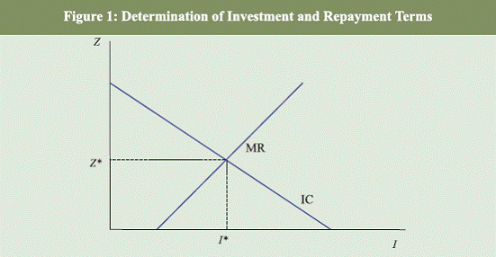An increase in debt is akin to a decline in the endowment of the borrower and shifts the MR curve to the left. The borrower relies more on external funds in this case which raises state contingent repayments given by Z_G .The inability of the borrower to guarantee a larger repayment in the bad state raises Z. Investment declines. Similarly, a rise in repudiation risk as given by a lower value of λ increases the inefficiency associated with formal default in the bad state and the higher default increases the expected interest repayment to the lender whilst still meeting their zero expected profit condition. The intuition is that given the presence of moral hazard the optimal financial contract calls for all available resources going to lenders in the situation where there is a low realisation of the output. A decrease in the repayment to lenders – a rise in λ - in the event of a low output realisation, increases the investment distortion due to moral hazard and reduces I. A GDP indexed bond avoids this inefficiency associated with formal default as lower debt repayments are agreed to in the event of lower realisations of output. This enables the borrower to undertake higher investment that still meets the zero expected profit condition of the lender.

1.3 : Stabilisation Properties

The effect of GDP indexed bonds is that they stabilise the path of the debt. Consider a floating rate bond with a coupon that varies with the performance of the economy. Then,

where, g_t = actual growth rate of the economy

g¯ = baseline growth rate of GDP, say the average of GDP growth rate over the previous 20 years

r¯ = coupon acceptable to investors when the country grows at the baseline rate

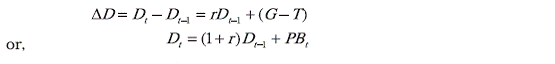
When the economy grows above the baseline rate the coupon rate will be higher than r% and will increase one for one with the growth rate of GDP. In the years when the economy grows below its baseline rate the coupon rate will be lower than r% but with a minimum of zero. We may write the budget constraint of the government as

The left-hand side of the above equation is the increase in the stock of debt which bears an interest rate of r or the fiscal deficit. The primary balance is the non-interest component of the fiscal deficit:

Another way of expressing the government-budget constraint is to write the budget constraint of the government in the following way:

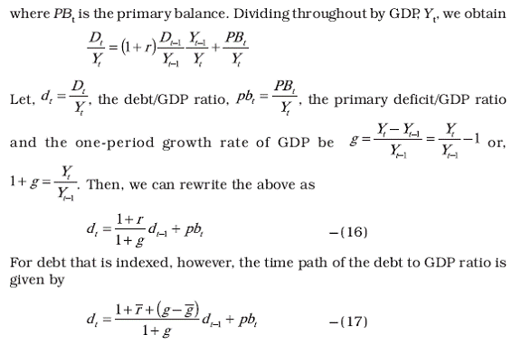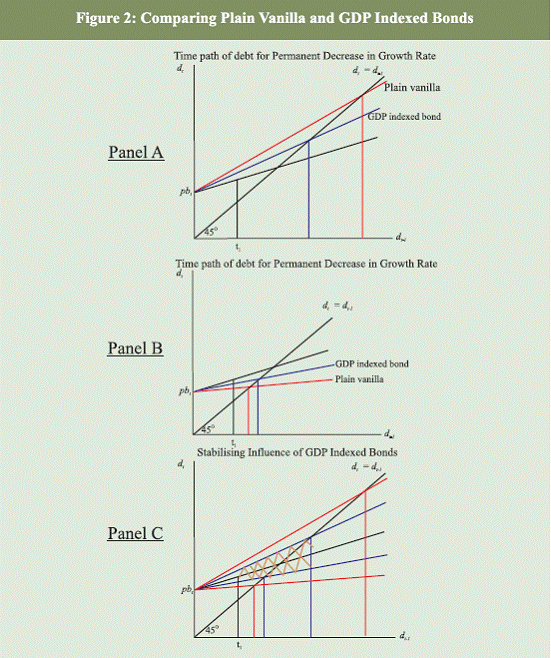
Comparing (16) with (17) we see that the decline in the debt/GDP ratio is smaller with a GDP indexed bond when the growth rate increases and vice versa. This effect of GDP indexed bonds is illustrated in Figure 2. Panel A of this figure depicts what happens to the debt to GDP ratio if there is a permanent decrease in the growth rate of GDP at time t₁. Then, if the debt were in the form of plain vanilla bonds, the debt/GDP ratio would grow faster than if the debt were in the form of GDP indexed bonds. Panel B depicts that if there were a permanent increase in the growth rate of GDP at time t₁, then, the debt/GDP ratio would grow slower if the debt were in the form of plain vanilla bonds than if the debt was in GDP indexed bonds. Finally Panel C shows the cross hatched area as the variation in the debt to GDP ratio when debt is in GDP indexed bonds which is lower than the variation as depicted by the outer cone when debt is in the form of plain vanilla bonds. The potential benefit of indexation can then be large if the primary deficit is taken to be constant.

1.4: Obstacles to Introducing GDP Indexed Bonds

Given the advantages of GDP indexed bonds many people consider it surprising as to why they have not been issued extensively. Some of the issues that have hindered the development of a market for such bonds include the following –

1. Accuracy of GDP data
2. Market illiquidity
3. Pricing difficulties

Of these the most important issue has been the difficulty in the pricing of GDP indexed bonds as it is an instrument with a more complicated structure than plain bonds. With regard to the accuracy of GDP data the major concern is about the quality of GDP data and that governments may deliberately misreport growth so as to affect the interest payments on growth indexed bonds. In this context it has been argued that to improve the transparency of the statistics the data should be verified or even provided by an external agency such as an international financial institution (Council of Economic Advisors, 2004). Sufficient liquidity in such instruments is also required to ensure they are traded frequently. Both issuer and investor appetite for these bonds could also be affected if there is a large premium required for them to be issued and picked up in the market in the first place. This may require active coordination by governments may be with the encouragement of international organisations to support several countries to issue such bonds at the same time so as to kick start a larger market for such instruments. These two issues of data and illiquidity are practical potential obstacles that require an institutional response whereas the issue of pricing is more a theoretical issue. We address this issue in the next section.

_______________

¹ The assumption that only period t + 1 consumption matters is a simplification which does not alter the results. Alternatively the borrower can be deemed to maximise representative lifetime utility.

Section II: Pricing Growth Indexed Bonds

Chamon and Mauro (2006; henceforth CM) advocate a Monte Carlo approach to pricing growth indexed bonds. Assuming risk neutral investors, they take advantage of the no arbitrage condition that the expected return on a bond issued by an emerging market borrower should equal the return on a bond issued by a developed country borrower (taken to be the US in CM). What follows is a description of the implementation of Monte Carlo using Indian data.

The first stage is calibration. This entails using the no arbitrage argument to extract the default trigger rate (the debt-GDP ratio, D_t / Y_t at which the default occurs) given the assumed recovery of principal (in the event of default) and the difference in observed yields in India and the US. Given the trigger rate, the next stage is pricing given the share of plain vanilla and growth-indexed portion in total debt.

II.1: Calibration

We directly list the steps below.

1. Debt Dynamics: The first step is specifying the stochastic process governing the evolution of debt-GDP ratio over time.

The following difference equation for dynamics results from the accounting relationship that debt at time t (D_t) is a sum of debt² at timet – 1, (D _t-1 ) the interest due and the primary deficit in the ensuing period:

4. Having specified the inputs and generated the sample paths, step four entails extracting the default trigger rate. This is done by exploiting the noarbitrage condition that expected return on an emerging market bond equals return on a bond with similar duration issued in the US.

Now there are multiple pairs of the default probability and recovery rate that can satisfy the no arbitrage constraint. For extracting the trigger rate implied by data, one of the two has to be assumed. Needless to say, assuming the baseline default probability defies the purpose.

We proceed as follows:

where the pre-specified θ now gives the level of indexation in the total debt issued. The coupon for the indexed portion is:

II.3: Inputs / Results

Input Values used at the Pricing Stage

At the pricing stage, we experiment with varying input values to see how sensitive results (total probability of default and the default trigger value) are to them. Table 1b lists the input values used at the pricing stage:

Other inputs like the risk free rate etc. are fixed at their values at the calibration stage (as in Table 1a above)

Results

II.4: Discussion of Results

First and foremost one observes in all the graphs that as indexation increases, payoff from the bond takes the shape of bell shape curve, indicating higher payments in case of higher growth and vice versa, although the exact nature depends on the value of other inputs, especially g*. Also, given other inputs, i.e. F_r, θ and p*, as g* goes up, one sees a ‘scale’ shift in the distribution to the right. For a stark affect compare the payoffs in the last panel (almost full indexation) of Figures 1a (or 2a or 3a) and Figure 1c (or 2c, or 3c).

As g* goes up, although the payout in terms of interest payments by the issuer (in this case the government) goes down, it also implies a slower growth in D_t / Y_t (one can think of g* as the strike price in a simple call/put option and government the writer of the option). This implies a lower total probability of default and thus, higher total payoff.

Although the effects of increasing g* are conflicting for the lender, it turns out that the effect of decrease in probability of default (and thus higher total payoff) outweighs the effect of likely higher coupon because of a lower ‘strike’. Needless to say, the larger the recovery rate, the lesser would be the impact (as in Figures 3a and 3c). As, while in the case of default, the total payoff is lower, a higher recovery rate implies that one gets a substantial part of the face value earlier in time (the present value effect).

The impact of changing p* is a little more straight-forward. As can be seen in equation [18], the higher the value of p*, the slower the growth rate D_t / Y_t , given the value of other inputs. Lower levels of D_t / Y_t implies a lower probability of default which in turn implies higher P(Trig*, Fr). Please see Tables 4a – 4c.

Also, as p* increases, the level of D_t / Y_t across all years goes down, and so must the default trigger level for the total expected discounted value to match par (100).

Although the baseline total probability of default f(Trig*, Fr) doesn’t depend g* on (no indexation at the calibration stage), the effect of increasing p* can be seen in Table 3 below.

Finally, in the spirit of CM we look at the result of changing p* and g* on the total probability of default with different levels of indexation, i.e. φ (Trig*, Fr, θ). CM in their study report these results only for ‘a’ given level of p* and g*.

For a given level of p*, for lower levels of g*, φ (Trig*, Fr, θ) increases with increasing indexation, θ. Only for higher levels of g*, does the impact go the other way round. It is only for higher g* (‘strike price’) that φ (Trig*, Fr, θ) decreases with increasing indexation. See Tables 5a – 5c.

What is happening on our understanding is that a higher g* implies a lower payout for the writer of the option, hence a lower probability of default with indexation.

Of course, results are (also) conditional on the given joint distribution of the random variables, g_t , ε_t and pb_t for a different country / dataset, results could be otherwise. The point to be noted is that, unless tested for, by looking at the joint distribution of the correlated random variables and values of other parameters, the impact is not obvious in one direction or the other. The only recourse is simulation. In the presence of randomness (esp. when one has to worry about how multiple random variable evolve jointly), a purely analytical framework can only take us as far.

II.5: Sensitivity Analysis

To validate the exercise, let’s see what happens when we change some of the free parameters (r_f , c₀ and α) in the model.

As a first consistency check, total expected payoff in the case of virtually no indexation (θ = 0.0001) should be very close to 100 (as during calibration). This is indeed the case, as seen in the 1st row of Tables 4a – 4c.

Sensitivity to changes in the value of free parameters can be assessed only in a ‘conditional’ sense, i.e. other inputs F_r , θ, p*, and g* will have to be fixed. This is done for the following case (close to currently observed values for p* and g* for India):

p* = 4%
g* = 7%
θ = 0.25
F_r = 25

Results are presented in Tables 6 – 8 and Figures 4 – 6, respectively for r_f , c₀ and α.

As r_ƒ increases, the discount rate to be applied for the payoff increases, implying a lower total expected payoff. So a higher default trigger value is needed (and correspondingly a lower total probability of default) to ensure that total payoff equals par.

Effect of increase in c₀ implies a higher payout in terms of interest payments which in turn implies a higher level of D_t / Y_t. This has two conflicting

effects, a higher payoff because of higher coupon payments but also a higher probability of default. The exact response would depend on the values of other inputs. Notice that till c_o = 7%, total expected payoff increases, and then decreases, indicating that higher probability of default dominates at very high c_o .

The effect of increasing share of foreign debt has a much lesser impact on the probability of default, and is relatively hard to explain unless one takes into account the distribution of change in real exchange rates in a particular scenario.

II.6: Some Observations on the Methodology and the Monte Carlo Exercise

All the qualitative results observed by CM are also observed in this study. However, this study goes further and provides in-depth results on various scenarios and sensitivity analysis to variation in free parameters.

The main observation is that in the case of indexation, not only that price of the indexed bond could be below par, but also the probability of default in case of indexation, φ (Trig*, Fr, θ) can increase, depending on the joint distribution of random variables g_t , ε_t and pb_t and value of other inputs to the model. Further, although qualitatively results are not very dissimilar to the ones provided by CM, exact distribution of payoff could be quantitatively substantially different depending on the value of the other inputs.

A limitation of this study is that the number of simulations considered for getting the distribution of payoffs and expected discounted value is on the lower side (1000). It is thus by no means prohibitive in getting a flavor of the issues in pricing growth indexed bonds.

Another relevant concern is that because of the strict restrictions on external (and so dollar denominated) borrowing, and investment by Indian residents abroad, the basic arbitrage condition used in the above approach is likely to have limited applicability in the present Indian context. Therefore, specifying the risk free interest rate equal to 4 per cent in the baseline computations, as in the CM approach, may be inappropriate.

While relevant, an “appropriate” risk number premium could be added to the risk free rate used for discounting, and this in spirit doesn’t change the ‘methodology’ of pricing GDP-indexed bonds.

In a similar vein, one could also argue against setting the coupon rate on plain vanilla bonds in the baseline computations equal to the average EMBI spread. However, the study does provide sensitivity results for varying coupon rates. In any case, choice of coupon rate on plain vanilla bonds would depend crucially on the interest rate environment, when and if, a central bank decides to issue growth-indexed bonds.

Another concern is that India has never so far defaulted on its external debt, with a currently very low ratio to GDP of the dollar denominated debt and of the short term external debt. In such a scenario an approach starting from the notion of a trigger value of debt GDP ratio may appear unconvincing if such a trigger value is not specified as dependent on the ratio of short term external debt to the stock of foreign exchange reserves. In our view, however, even setting a trigger value to be dependent on the external debt/foreign exchange reserves ratio is meaningless in a world of capital flows.

Many would also like to understand the role of GDP indexed bonds in the context of a bond market such as India’s, which is largely dominated at present by domestic investors, in terms of stabilising government finances and debt and possibly lowering the cost of government borrowing. The issuing of such bonds in a domestic context would require us to address larger issues such as the role of sovereign default in a purely domestic context. The ex post possibility of default may be ex ante efficient in encouraging sovereigns to repay their obligations and indeed make it possible for sovereign debt markets to exist in the first place. There are also institutional factors one would have to consider such as the absence of legal recourse available to creditors to enforce payments when sovereign obligations are not honoured and the implications for such instruments when the market for government securities is propped by mandated investment requirements on bank and other financial institution portfolios. More importantly market liquidity in the government securities market is fairly limited, with most government bonds held to maturity. These issues are outside the scope of the study.
_______________

² Debt here refers to the total government debt

³ Inflation “target” here refers to the US target for the medium term – in line with CM’s usage.

⁴ Selection of the “target” growth rate is taken to be something exogenous to the study. We think that when, and if a central bank such as the RBI decides to go through with such an initiative, appropriate inflation, coupon, growth targets will have to be decided upon – something which we believe RBI as a central bank is much better placed than the authors of the study. This study is predominantly illustrative of what such choices entail for such instruments.

⁵ One could argue that strategy of using the small sample to generate the correlated random variables is ‘flawed’. However, ‘desired’/’actual’ properties of the random variables can be simulated. From a practical point of view, it’s an easy enough task, and not central to the study. As it is, in principle, it doesn’t cause any change in the methodology.

⁶ Finer step-sizes can be selected too. But, for illustrative purposes, 1/10th of a percent is good enough.

⁷ In particular, we found that no-default became a certainty on all sample paths. What we think could be happening is that, a higher implies a lower D_t / Y_t , and consequently a less likely default. From a more practical point of view, most developed country central banks do have ‘medium level inflation targets’ that hover around 2%, including the US.

⁸ Recall that the trigger level (Trig*) is an output from the calibration exercise

Section III: Concluding Remarks

This paper has analysed what GDP indexed bonds achieve, their stabilisation properties, and the obstacles to the introduction of such bonds especially in terms of pricing of such bonds. We do not see the commonly stated obstacles as insurmountable. We, however, believe there are practical issues involved in the issue of such instruments which reduce their desirability in the Indian context. The main one in the Indian context is that the introduction of such a financial instrument requires offering a premium to hold it as investors are uncertain about a new instrument. As GDP indexed bonds make a substantial difference only when they have a long term maturity of five years or more it is not easy for an incumbent government to issue such bonds that make life easier for their successors. Moreover when an economy is going through a buoyant growth phase it makes it difficult for a Finance Minister to justify payment of an insurance premium and higher coupons. Such bonds have so far been introduced in the world economy in Costa Rica, Bulgaria, Bosnia and Herzegovina, and Argentina, as part of a debt restructuring programme. Their attractiveness when an economy’s productivity growth rate increases as currently is the case in India is in doubt as investors may read an ambiguous signal with the introduction of such an instrument in the current buoyant phase. Issues of such an instrument cannot be made in small tranches as sufficient liquidity is important for them to be actively traded and held. The estimates of savings for the economy that Borensztein and Mauro (2004) give for Mexico for instance require that half of the debt should have been in the form of GDP indexed bonds for the country to have saved a little over 1 per cent of GDP in interest payments during the 1995 crisis. Thus it seems such bonds will be more successful if they are issued by different emerging markets, instead of one coming as it would make it easier for investors to make comparisons and to make price discovery possible. This requires coordination at an international level, that is a public good which no one country will find profitable to undertake.

Substantially also these bonds are a response to the presence of moral hazard due to the existence of repudiation risk. In that case there may be a tradeoff between attempting to complete the financial markets with such instruments and promoting institutions that deepen the market and make them more liquid. Countries that promote political stability, trade openness, the rule of law, etc. reduce repudiation risk and at the same time ameliorate the adverse incentive effects of moral hazard and improve access to capital markets. GDP indexed bonds play a similar role – they eliminate the inefficiencies arising from formal default and maximize the incentive to invest. Sound institutions and policies may be as effective in reducing risk and make debt sustainable.

A GDP indexed bond would be valuable when an economy is unable to credibly commit to sound fiscal policies which then leaves investors less willing to supply capital to an economy. By reducing the risk of repayment such a financial instrument attempts to keep investors confident and keep capital flows to the economy sustainable. However, arguably instituting credible fiscal policy may be more beneficial to handling the risk that is being sought to be addressed. One such institution is the legislation of fiscal rules that have teeth in the form of penalties in case the government does not meet the targets set by such rules. These rules could be in the form of expenditure limiting rules, overall balance rules prescribing limits to fiscal deficits, and public debt rules. In some cases it may even be advisable to institute an independent fiscal authority that has the power to set the permissible change in the public debt which it sets by taking into consideration that budget deficits now would be offset by surpluses in the future. This gives a long term perspective to fiscal policy than that offered by a government which may be out of office tomorrow and is tempted to manipulate the deficit so as to increase its chances of re-election. The members of such an autonomous authority which is established by law would have to be appointed for long and staggered terms in office with a mandate to insure the stability of public finance. They would set limits to public debt not on the basis of rules but on the basis of sustainability of the debt. The decision about the size of government and about taxation would however still be with the executive and legislative branches of government. Such institutions address problems of commitment and play the role of monitoring and signaling government performance on the fiscal front. In emerging markets it may be more sensible to deepen institutions and make policies that are sustainable rather than attempt to address financial market inefficiencies through the use of financial engineering.

References

Atkeson, Andrew (1991) – “International Lending with Moral Hazard and Risk of Repudiation”, Econometrica, 59, 1069 – 89.

Bernanke, B. and M. Gertler (1989) – “Agency Costs, Net Worth and Business Fluctuations”, American Economic Review, 79, 14 – 31.

Borensztein, E. and P. Mauro (2004) – “The Case for GDP – Indexed Bonds”, Economic Policy, April, 165 – 216.

Campbell, J.Y. and R.J. Shiller (1996) – “A Scorecard for Indexed Government Debt”, NBER Macroeconomics Annual, 155 – 97.

Chamon, M. and P. Mauro (2006) – “Pricing Growth-Indexed Bonds”, Journal of Banking & Finance, XXX, 1 – 18.

Council of Economic Advisers (2004) – “Growth – Indexed Bonds: A primer”, July 8, Washington DC. [http://www.whitehouse.gov /cea/growth-indexedbonds-white-paper.pdf]

Eaton, J. and M. Gersowitz (1981) – “Debt with Potential Repudiation: Theory and Estimation”, Review of Economic Studies, 48, 289 – 309.

Froot, K.A., D.S. Scharsfstein, and J. Stein (1989) – “LDC Debt: Forgiveness, Indexation, and Investment Incentives”, Journal of Finance, 44(5), 1335 – 50.

Gertler, M. and K. Rogoff (1990) – “North-South Lending and Endogenous Capital Market Inefficiencies”, Journal of Monetary Economics, 26, 245 – 66.

Griffith-Jones, S. and K. Sharma (2006) – “GDP – Indexed Bonds: Making it Happen”, UN Department of Economic and Social Affairs Working Paper No. 21, ST/ESA/2006/DWP/21.

Krugman, P. (1988) – “Financing vs. Forgiving a Debt Overhang”, Journal of Development Economics, 29, 253 – 68.

Lane, Philip R. (1999) – “North – South Lending with Moral Hazard and Repudiation Risk”, Review of International Economics, 7(1), 50 – 58.

Appendix