|
ACKNOWLEDGEMENTS
We are deeply indebted to Dr. Rakesh Mohan, former Deputy
Governor, for giving us the opportunity to undertake this project.
We are also very grateful to Dr. R.K. Pattnaik, former Adviser,
Department of Economic Analysis and Policy (DEAP), for insightful
discussions and support throughout the project. We are thankful to DRG for
the excellent support rendered to us during the course of the study.
The authors also gratefully acknowledge insightful inputs and
suggestions from Sangita Misra, Harendra Behera, Binod B. Bhoi, Vijay
Raina and Meena Ravichandran from the Reserve Bank of India. Special
thanks are also due to Ganesh Manjhi, Chhanda Mandal and Reetika Garg
for competent research assistance.
We also gratefully acknowledge constructive comments and suggestions
from two anonymous referees. The external expert also acknowledges a
research grant from the Research and Development Programme of the
University of Delhi awarded in the preliminary stages of this research.
A large part of the research was conducted when the external expert
was Visiting Professor at the Dayalbagh Educational Institute (Deemed
University), Agra. The external expert gratefully acknowledges support from
the Institute during the course of this study.
Finally, we acknowledge that we are solely responsible for errors,
if any.
Pami Dua and Rajiv Ranjan
ABBREVIATIONS
VAR |
Vector Autoregressive |
BVAR |
Bayesian vector autoregressive |
ADs |
Authorised Dealers |
FERA |
Foreign Exchange Regulations Act |
LERMS |
Liberalized Exchange Rate Management System |
FEMA |
Foreign Exchange Management Act |
CCIL |
Clearing Corporation of India Limited |
MSS |
Market Stabilisation Scheme |
KYC |
Know-Your-Customer |
ECB |
External Commercial Borrowings |
FEDAI |
Foreign Exchange Dealers’ Association of India |
CCIL |
Clearing Corporation of India Ltd. |
MCX-SX |
Multi Commodity Exchange – Stock Exchange |
RMDS |
Reuters Market Data System |
OTC |
Over The Counter |
BIS |
Bank for International Settlements |
IOC |
Indian Oil Corporation |
NDF |
Non Deliverable Forward |
EMEs |
Emerging Market Economies |
FIIs |
Foreign Institutional Investors’ |
FDI |
Foreign Direct Investment |
LAF |
Liquidity Adjustment Facility |
OMO |
Open Market Operations |
MSS |
Market Stabilisation Scheme |
FCA |
Foreign Currency Assets |
PPP |
Purchasing Power Parity |
PBM |
Portfolio Balance Model |
VECM |
Vector Error Correction Model |
MSIH |
Markov Switching Intercept Heteroscedastic |
RMSE |
Root Mean Square Error |
EXECUTIVE SUMMARY
The exchange rate is a key financial variable that affects decisions
made by foreign exchange investors, exporters, importers, bankers,
businesses, financial institutions, policymakers and tourists in the
developed as well as developing world. Exchange rate fluctuations affect
the value of international investment portfolios, competitiveness of exports
and imports, value of international reserves, currency value of debt
payments, and the cost to tourists in terms of the value of their currency.
Movements in exchange rates thus have important implications for the
economy’s business cycle, trade and capital flows and are therefore crucial
for understanding financial developments and changes in economic policy.
The study covers two main topics: first, various aspects of economic
policy with respect to the exchange rate, and second, modeling and
forecasting the exchange rate. Accordingly, the study analyses India’s
exchange rate story and discusses the structure of the foreign exchange
market in India in terms of participants, instruments and trading platform
as also turnover in the Indian foreign exchange market and forward
premia. The Indian foreign exchange market has evolved over time as a
deep, liquid and efficient market as against a highly regulated market
prior to the 1990s. The market participants have become sophisticated,
the range of instruments available for trading has increased, the turnover
has also increased, while the bid–ask spreads have declined. This study
also covers the exchange rate policy of India in the background of large
capital flows,
The study then attempts to develop a model for the rupee-dollar
exchange rate taking into account variables from monetary and micro
structure models as well as other variables including intervention by the
central bank. The focus is on the exchange rate of the Indian rupee vis-àvis
the US dollar, i.e., the Re/$ rate. To model the exchange rate, the monetary
model is expanded to include variables that may have been important in
determining exchange rate movements in India such as forward premia,
capital flows, order flows and central bank intervention.
Exchange Rates and Exchange Rate Policy in India: A Review
India’s exchange rate policy has evolved over time in line with the
gradual opening up of the economy as part of the broader strategy of
macroeconomic reforms and liberalization since the early 1990s. In the
post independence period, India’s exchange rate policy has seen a shift
from a par value system to a basket-peg and further to a managed float
exchange rate system. With the breakdown of the Bretton Woods System in
1971, the rupee was linked with pound sterling. In order to overcome the
weaknesses associated with a single currency peg and to ensure stability of
the exchange rate, the rupee, with effect from September 1975, was pegged
to a basket of currencies till the early 1990s.
The initiation of economic reforms saw, among other measures, a two
step downward exchange rate adjustment by 9 per cent and 11 per cent
between July 1 and 3, 1991 to counter the massive draw down in the
foreign exchange reserves, to install confidence in the investors and to
improve domestic competitiveness. The Liberalised Exchange Rate
Management System (LERMS) was put in place in March 1992 involving
the dual exchange rate system in the interim period. The dual exchange
rate system was replaced by a unified exchange rate system in March 1993.
The experience with a market determined exchange rate system in India
since 1993 is generally described as ‘satisfactory’ as orderliness prevailed
in the Indian market during most of the period. Episodes of volatility were
effectively managed through timely monetary and administrative measures.
An important aspect of the policy response in India to the various
episodes of volatility has been market intervention combined with monetary
and administrative measures to meet the threats to financial stability while
complementary or parallel recourse has been taken to communications
through speeches and press releases. In line with the exchange rate policy,
it has also been observed that the Indian rupee is moving along with the
economic fundamentals in the post-reform period. Moving forward, as India
progresses towards full capital account convertibility and gets more and
more integrated with the rest of the world, managing periods of volatility is bound to pose greater challenges in view of the impossible trinity of
independent monetary policy, open capital account and exchange rate
management. Preserving stability in the market would require more
flexibility, adaptability and innovations with regard to the strategy for
liquidity management as well as exchange rate management. With the likely
turnover in the foreign exchange market rising in future, further
development of the foreign exchange market will be crucial to manage the
associated risks.
Structure of the Indian Foreign Exchange Market and Turnover
Prior to the 1990s, the Indian foreign exchange market (with a pegged
exchange rate regime) was highly regulated with restrictions on transactions,
participants and use of instruments. The period since the early 1990s has
witnessed a wide range of regulatory and institutional reforms resulting in
substantial development of the rupee exchange market as it is observed
today. Market participants have become sophisticated and have acquired
reasonable expertise in using various instruments and managing risks.
The foreign exchange market in India today is equipped with several
derivative instruments. Various informal forms of derivatives contracts have
existed since time immemorial though the formal introduction of a variety
of instruments in the foreign exchange derivatives market started only in
the post reform period, especially since the mid-1990s. These derivative
instruments have been cautiously introduced as part of the reforms in a
phased manner, both for product diversity and more importantly as a risk
management tool. Recognising the relatively nascent stage of the foreign
exchange market then with the lack of capabilities to handle massive
speculation, the ‘underlying exposure’ criteria had been imposed as a
prerequisite.
Trading volumes in the Indian foreign exchange market has grown
significantly over the last few years. The daily average turnover has seen
almost a ten-fold rise during the 10 year period from 1997-98 to 2007-08
from US $ 5 billion to US $ 48 billion. The pickup has been particularly sharp from 2003-04 onwards since when there was a massive surge in
capital inflows. It is noteworthy that the increase in foreign exchange market
turnover in India between April 2004 and April 2007 was the highest
amongst the 54 countries covered in the latest Triennial Central Bank Survey
of Foreign Exchange and Derivatives Market Activity conducted by the Bank
for International Settlements (BIS). According to the survey, daily average
turnover in India jumped almost 5-fold from US $ 7 billion in April 2004
to US $ 34 billion in April 2007; global turnover over the same period rose
by only 66 per cent from US $ 2.4 trillion to US $ 4.0 trillion. Reflecting
these trends, the share of India in global foreign exchange market turnover
trebled from 0.3 per cent in April 2004 to 0.9 per cent in April 2007. With
the increasing integration of the Indian economy with the rest of the world,
the efficiency in the foreign exchange market has improved as evident from
low bid-ask spreads. It is found that the spread is almost flat and very low.
In India, the normal spot market quote has a spread of 0.25 paisa to 1
paise while swap quotes are available at 1 to 2 paise spread. Thus, the
foreign exchange market has evolved over time as a deep, liquid and efficient
market as against a highly regulated market prior to the 1990s.
Capital Flows and Exchange Rates: The Indian Experience
In the recent period, external sector developments in India have been
marked by strong capital flows, which had led to an appreciating tendency
in the exchange rate of the Indian rupee up to January 2008. The movement
of the Indian rupee is largely influenced by the capital flow movements
rather than traditional determinants like trade flows. Though capital flows
are generally seen to be beneficial to an economy, a large surge in flows
over a short span of time in excess of the domestic absorptive capacity
can, however, be a source of stress to the economy giving rise to upward
pressures on the exchange rate, overheating of the economy, and possible
asset price bubbles.
In India, the liquidity impact of large capital inflows was traditionally
managed mainly through the repo and reverse repo auctions under the day-to-day Liquidity Adjustment Facility (LAF). The LAF operations were
supplemented by outright open market operations (OMO), i.e. outright sales
of the government securities, to absorb liquidity on an enduring basis. In
addition to LAF and OMO, excess liquidity from the financial system was
also absorbed through the building up of surplus balances of the
Government with the Reserve Bank, particularly by raising the notified
amount of 91-day Treasury Bill auctions, and forex swaps. In view of the
large capital flows during the past few years, relaxations were effected in
regard to outflows, both under the current and capital accounts. In addition,
changes in policies are made from time to time to modulate the debt-creating
capital flows depending on the financing needs of the corporate sector and
vulnerability of the domestic economy to external shocks.
In the face of large capital flows coupled with declining stock of
government securities, the Reserve Bank of India introduced a new instrument
of sterilisation, viz., the Market Stabilisation Scheme (MSS) to sustain market
operations. Since its introduction in April 2004, the MSS has served as a
very useful instrument for medium term monetary and liquidity management.
The cost of sterilisation in India is shared by the Central Government (the
cost of MSS), Reserve Bank (sterilization under LAF) and the banking system
(in case of increase in the reserve requirements).
With the surge in capital flows to EMEs, issues relating to management
of those flows have assumed importance as they have bearings on the
exchange rates. Large capital inflows create important challenges for
policymakers because of their potential to generate overheating, loss of
competitiveness, and increased vulnerability to crisis. Reflecting these
concerns, policies in EMEs have responded to capital inflows in a variety
of ways. While some countries have allowed the exchange rate to appreciate,
in many cases monetary authorities have intervened heavily in forex markets
to resist currency appreciation. EMEs have sought to neutralize the
monetary impact of intervention through sterilization. Cross-country
experiences reveal that in the recent period most of the EMEs have adopted
a more flexible exchange rate regime.
In view of the importance of capital flows, foreign exchange intervention
and turnover in determination of exchange rates, these variables are
included in the modeling exercise undertaken to analyze the behaviour of
the exchange rate.
Modelling and Forecasting the Re/$ Exchange Rate: Economic Theory
and Review of Literature
In the international finance literature, various theoretical models are
available to analyze exchange rate determination and behaviour. Most of
the studies on exchange rate models prior to the 1970s were based on the
fixed price assumption1. With the advent of the floating exchange rate regime
amongst major industrialized countries in the early 1970s, an important
advance was made with the development of the monetary approach to
exchange rate determination. The dominant model was the flexible-price
monetary model that has been analyzed in many early studies like Frenkel
(1976), Mussa (1976, 1979), Frenkel and Johnson (1978), and more
recently by Vitek (2005), Nwafor (2006), Molodtsova and Papell, (2007).
Following this, the sticky price or overshooting model by Dornbusch (1976,
1980) evolved, which has been tested, amongst others, by Alquist and Chinn
(2008) and Zita and Gupta (2007). The portfolio balance model also
developed alongside2 , which allowed for imperfect substitutability between
domestic and foreign assets, and considered wealth effects of current
account imbalances.
With liberalization and development of foreign exchange and assets
markets, variables such as capital flows, volatility in capital flows and
forward premium have also became important in determining exchange
rates. Furthermore, with the growing development of foreign exchange
markets and a rise in the trading volume in these markets, the micro level
dynamics in foreign exchange markets increasingly became important in determining exchange rates. Agents in the foreign exchange market have
access to private information about fundamentals or liquidity, which is
reflected in the buying/selling transactions they undertake, that are termed
as order flows (Medeiros, 2005; Bjonnes and Rime, 2003). Microstructure
theory evolved in order to capture the micro level dynamics in the foreign
exchange market (Evans and Lyons, 2001, 2005, 2007). Another variable
that is important in determining exchange rates is central bank intervention
in the foreign exchange market.
Non-linear models have also been considered in the literature. Sarno
(2003), Altaville and Grauwe (2006) are some of the recent studies that
have used non-linear models of the exchange rate.
Overall, forecasting the exchange rates has remained a challenge for
both academicians as well as market participants. In fact, Meese and Rogoff’s
seminal study (1983) on the forecasting performance of the monetary models
demonstrated that these failed to beat the random walk model. This has
triggered a plethora of studies that test the superiority of theoretical and
empirical models of exchange rate determination vis-a-vis a random walk.
In sum, several exchange rate models available in the literature have
been tested during the last two and a half decades. No particular model
seems to work best at all times/horizons. Monetary models based on the
idea of fundamentals’ driven exchange rate behaviour work best in the
long-run, but lose their predictability in the short-run to naïve random
walk forecasts. The volatility of exchange rates also substantially exceeds
that of the volatility of macroeconomic fundamentals, thus providing further
evidence of weakening fundamental-exchange rate link. A combination of
the different monetary models, however, at times gives better results than
the random walk. Order flows also play an important role in influencing
the exchange rate. Keeping in view all the above results of the literature,
this study attempts to develop a model for the rupee-dollar exchange rate
taking into account all the different monetary models along with the
microstructure models incorporating order flow, as well as capital flows,
forward premium and central bank intervention.
Modelling and Forecasting the Exchange Rate: Econometric
Methodology, Estimation, Evaluation and Findings
This study attempts to gauge the forecasting ability of economic models
with respect to exchange rates with the difference that this is done in the
context of a developing country that follows a managed floating (as opposed
to flexible) exchange rate regime. Starting from the naïve model, this study
examines the forecasting performance of the monetary model and various
extensions of it in the vector autoregressive (VAR) and Bayesian vector
autoregressive (BVAR) framework. Extensions of the monetary model
considered in this study include the forward premium, capital inflows,
volatility of capital flows, order flows and central bank intervention. The
study therefore examines, first, whether the monetary model can beat a
random walk. Second, it investigates if the forecasting performance of the
monetary model can be improved by extending it. Third, the study evaluates
the forecasting performance of a VAR model vs a BVAR model. Lastly, it
considers if information on intervention by the central bank can improve
forecast accuracy. The main findings are as follows :
(i) The monetary model generally outperforms the naïve model. This
negates the findings of the seminal study by Meese and Rogoff (1983)
that finds that models which are based on economic fundamentals
cannot outperform a naive random walk model.
(ii) The result that it is possible to beat the naïve model may be due to the
fact that the intervention by the central bank may help to curb volatility
arising due to demand-supply mismatch and stabilize the exchange
rate. The exchange rate policy of the RBI is guided by the need to
reduce excess volatility. The Reserve Bank has been prepared to make
sales and purchases of foreign currency in order to even out lumpy
demand and supply in the relatively thin foreign exchange market and
to smoothen jerky movements.
(iii) Forecast accuracy can be improved by extending the monetary model
to include forward premium, volatility of capital inflows and order flow.
(iv) Information on intervention by the central bank helps to improve
forecasts at the longer end.
(v) Bayesian vector autoregressive models generally outperform their
corresponding VAR variants.
(vi) Turning points are difficult to predict as illustrated using Model 4
with predictions made in February 2008.
Thus, availability of information on certain key variables at regular
intervals that affect the exchange rate can lead to a more informed view
about the behavior of the future exchange rates by the market participants,
which may allow them to plan their foreign exchange exposure better by
hedging them appropriately. Such key variables could include past data on
exchange rates, forward premia, capital flows, turnover, and intervention
by central banks etc. As regards availability of data on key variables relating
to the Indian foreign exchange market, most of the data are available in
public domain and can easily be accessed by market participants,
academicians and professional researchers. Using these variables skillfully
will help them to gain sound insight into future exchange rate movements.
In this context, it is important to recognize that the Indian approach
in recent years has been guided by the broad principles of careful monitoring
and management of exchange rates with flexibility, without a fixed target or
a pre-announced target or a band, coupled with the ability to intervene if
and when necessary, while allowing the underlying demand and supply
conditions to determine the exchange rate movements over a period in an
orderly way. Subject to this predominant objective, the exchange rate policy
is guided by the need to reduce excess volatility, prevent the emergence of
establishing speculative activities, help maintain adequate level of reserves,
and develop an orderly foreign exchange market.
1 See e.g. Marshall (1923), Lerner (1936), Nurkse (1944), Harberger (1950), Mundell (1961, 1962, 1963)
and Fleming (1962).
2 See e.g. Dornbusch and Fischer (1980), Isard (1980), Branson (1983, 1984).
EXCHANGE RATE POLICY AND MODELLING
IN INDIA
Pami Dua, Rajiv Ranjan*
SECTION I
Introduction
The exchange rate is a key financial variable that affects decisions
made by foreign exchange investors, exporters, importers, bankers,
businesses, financial institutions, policymakers and tourists in the
developed as well as developing world. Exchange rate fluctuations affect
the value of international investment portfolios, competitiveness of
exports and imports, value of international reserves, currency value of
debt payments, and the cost to tourists in terms of the value of their
currency. Movements in exchange rates thus have important implications
for the economy’s business cycle, trade and capital flows and are therefore
crucial for understanding financial developments and changes in
economic policy. Timely forecasts of exchange rates can therefore provide
valuable information to decision makers and participants in the spheres
of international finance, trade and policy making. Nevertheless, the
empirical literature is skeptical about the possibility of accurately
predicting exchange rates.
In the international finance literature, various theoretical models
are available to analyze exchange rate behaviour. While exchange rate
models existed prior to 1970s (Nurkse, 1944; Mundell, 1961, 1962,
1963), most of them were based on the fixed price assumption. With
the advent of the floating exchange rate regime amongst major
industrialized countries in the early 1970s, a major advance was made
with the development of the monetary approach to the exchange rate
determination. The dominant model was the flexible price monetary
model that gave way to the sticky price and portfolio balance model.
While considerable amount of empirical work was devoted to testing
these monetary models, most of them focused on in-sample tests that
do not really give the true predictive accuracy of the models. Following
this, the sticky price or overshooting model by Dornbusch (1976, 1980) evolved, which has been tested, amongst others, by Alquist and Chinn
(2008) and Zita and Gupta (2007). The portfolio balance model also
developed alongside , which allowed for imperfect substitutability
between domestic and foreign assets, and considered wealth effects of
current account imbalances.
With liberalization and development of foreign exchange and assets
markets, variables such as capital flows, volatility in capital flows and
forward premium have also became important in determining exchange
rates. Furthermore, with the growing development of foreign exchange
markets and a rise in the trading volume in these markets, the micro
level dynamics in foreign exchange markets have increasingly became
important in determining exchange rates. Agents in the foreign exchange
market have access to private information about fundamentals or
liquidity, which is reflected in the buying/selling transactions they
undertake, that are termed as order flows (Medeiros, 2005; Bjonnes
and Rime 2003). Thus microstructure theory evolved in order to capture
the micro level dynamics in the foreign exchange market (Evans and
Lyons, 2001, 2005, 2007). Another variable that is important in determining
exchange rates is central bank intervention in the foreign exchange
market.
Non-linear models have also been considered in the literature. Sarno
(2003), Altaville and Grauwe (2006) are some of the recent studies that
have used non-linear models of the exchange rate.
This study attempts to develop a model for the rupee-dollar exchange
rate taking into account the different monetary models along with the
micro structure models incorporating order flow as well as other variables
including intervention by the central bank. The focus is on the exchange
rate of the Indian rupee vis-à-vis the US dollar, i.e., the Re/$ rate.
India has been operating on a managed floating exchange rate regime
from March 1993, marking the start of an era of a market determined
exchange rate regime of the rupee with provision for timely intervention by the central bank1
. India’s exchange rate policy has evolved overtime in
line with the global situation and as a consequence to domestic
developments. 1991-92 represents a major break in policy when India
harped on reform measures following the balance of payments crisis and
shifted to a market determined exchange rate system. As has been the
experience with the exchange rate regimes the world over, the Reserve Bank
as the central bank of the country has been actively participating in the
market dynamics with a view to signaling its stance and maintaining orderly
conditions in the foreign exchange market. The broad principles that have
guided India’s exchange rate management have been periodically articulated
in the various Monetary Policy Statements. These include careful monitoring
and management of exchange rates with flexibility, no fixed target or a preannounced
target or a band and ability to intervene, if and when necessary.
Based on the preparedness of the foreign exchange market and India’s
position on the external front (in terms of reserves, debt, current account
deficit etc), reform measures have been progressively undertaken to have a
liberalized exchange and payments system for current and capital account
transactions and further to develop the foreign exchange market.
This study covers two main topics: first, various aspects of economic
policy with respect to the exchange rate, second, modelling and forecasting
the exchang rate. Accordingly, this study analyses India’s exchange rate
story, with particular focus on the policy responses during difficult times
and the reforms undertaken to develop the rupee exchange market during
relatively stable times. This study also discusses the structure of the
foreign exchange market in India in terms of participants, instruments
and trading platform as also turnover in the Indian foreign exchange market and forward premia. The Indian foreign exchange market has
evolved over time as a deep, liquid and efficient market as against a
highly regulated market prior to the 1990s. The market participants
have become sophisticated, the range of instruments available for trading
has increased, the turnover has also increased, while the bid–ask spreads
have declined. This study also covers the exchange rate policy of India in
the background of large capital flows, in terms of their magnitude,
composition and management. In the recent period, up to 2007-08,
external sector developments in India have been marked by strong capital
inflows. Capital flows to India, which were earlier mainly confined to
small official concessional finance, gained momentum from the 1990s
after the initiation of economic reforms.
After studying the analytics of foreign exchange market and the factors
affecting the exchange rate in the first part of the study (Sections II, III
and IV), this study then in the second part attempts to gauge the
forecasting ability of economic models with respect to exchange rates in
the context of a developing country that follows a managed floating (as
opposed to flexible) exchange rate regime. Starting from the naïve model,
this study examines the forecasting performance of the monetary model
and various extensions of it in the vector autoregressive (VAR) and
Bayesian vector autoregressive (BVAR) framework. Extensions of the
monetary model considered in this study include the forward premium,
capital inflows, volatility of capital flows, order flows and central bank
intervention. The study therefore examines, first, whether the monetary
model can beat a random walk. Second, it investigates if the forecasting
performance of the monetary model can be improved by extending it.
Third, the study evaluates the forecasting performance of a VAR model
versus a BVAR model. Lastly, it considers if information on intervention
by the central bank can improve forecast accuracy.
This study concentrates on the post March 1993 period and provides
insights into forecasting exchange rates for developing countries where
the central bank intervenes periodically in the foreign exchange market.
The alternative forecasting models are estimated using monthly data from July 1996
2
to December 2006 while out-of-sample forecasting
performance is evaluated from January 2007 to June 2008. This study
negates the finding of the seminal Study by Meese and Rogoff (1983) that
models which are based on economic fundamentals cannot outperform
a naive random walk model.
Against this backdrop, Section II of this study presents a review of
exchange rates and exchange rate policy in India during different phases.
In Section III, the structure of the foreign exchange market in India,
turnover and forward premia are discussed in detail. This is followed by
a discussion on capital flows and the foreign exchange market in Section
IV. The economic theory and review of literature are covered in Section
V, while the econometric methodology is discussed in Section VI. The
estimation and evaluation of forecasting models is done in Section VII.
The last Section VIII presents some concluding observations.
SECTION II
Exchange Rates and Exchange Rate Policy in India: A Review
India’s exchange rate policy has evolved over time in line with the
gradual opening up of the economy as part of the broader strategy of
macroeconomic reforms and liberalization since the early 1990s. This
change was also warranted by the consensus response of all major
countries to excessive exchange rate fluctuations that accompanied the
abolishment of fixed exchange rate system. The major changes in the
exchange rate policy started with the implementation of the
recommendations of the High Level Committee on Balance of Payments
(Chairman: Dr. C. Rangarajan, 1993) to make the exchange rate marketdetermined.
The Expert Group on Foreign Exchange Markets in India
(popularly known as Sodhani Committee, 1995) made several
recommendations with respect to participants, trading, risk management as well as selective market intervention by the Reserve Bank to promote
greater market development in an orderly fashion. Consequently, the
period starting from January 1996 saw wide-ranging reforms in the Indian
foreign exchange market. In essence, the exchange rate developments
changed in side-by-side with the reform in the external sector of India.
With the external sector reform, India stands considerably integrated
with the rest of the world today in terms of increasing openness of the
economy. As a result of calibrated and gradual capital account openness,
the financial markets, particularly forex market, in India have also
become increasingly integrated with the global network since 2003-04.
This is reflected in the extent and magnitude of capital that has flown
to India in recent years. Exchange rates exhibited considerable volatility
and increased capital mobility has posed several challenges before the
monetary authorities in managing exchange rates.
Against this backdrop, the following section analyses in retrospect
India’s exchange rate story, with particular focus on the policy responses
during difficult times and the reforms undertaken to develop the rupee
exchange market during relatively stable times.
1. Chronology of Reform Measures
In the post independence period, India’s exchange rate policy has
seen a shift from a par value system to a basket-peg and further to a
managed float exchange rate system. During the period 1947 till 1971,
India followed the par value system of the exchange rate whereby the
rupee’s external par value was fixed at 4.15 grains of fine gold. The RBI
maintained the par value of the rupee within the permitted margin of
±1% using pound sterling as the intervention currency. The devaluation
of the rupee in September 1949 and June 1966 in terms of gold resulted
in the reduction of the par value of rupee in terms of gold to 2.88 and
1.83 grains of fine gold, respectively. Since 1966, the exchange rate of
the rupee remained constant till 1971 (Chart 2.1).
 |
With the breakdown of the Bretton Woods System, in December 1971,
the rupee was linked with pound sterling. Sterling being fixed in terms
of US dollar under the Smithsonian Agreement of 1971, the rupee also
remained stable against dollar. In order to overcome the weaknesses
associated with a single currency peg and to ensure stability of the
exchange rate, the rupee, with effect from September 1975, was pegged
to a basket of currencies (Table 2.1). The currencies included in the
basket as well as their relative weights were kept confidential by the
Reserve Bank to discourage speculation.
By the late ‘eighties and the early ‘nineties, it was recognised that
both macroeconomic policy and structural factors had contributed to
balance of payment difficulties. The current account deficit widened to
3.0 per cent of GDP in 1990-91 and the foreign currency assets depleted
to less than a billion dollar by July 1991. It was against this backdrop
that India embarked on stabilisation and structural reforms to generate
impulses for growth.
Table 2.1 : Chronology of the Indian Exchange Rate |
Year |
The Foreign Exchange Market and Exchange Rate |
1947-1971 |
Par Value system of exchange rate. Rupee’s external par value was fixed in
terms of gold with the pound sterling as the intervention currency. |
1971 |
Breakdown of the Bretton-Woods system and floatation of major currencies. Rupee was linked to the pound sterling in December 1971. |
1975 |
To ensure stability of the Rupee, and avoid the weaknesses associated with a single currency peg, the Rupee was pegged to a basket of currencies. Currency selection and weight assignment was left to the discretion of the RBI and not publicly announced. |
1978 |
RBI allowed the domestic banks to undertake intra-day trading in foreign exchange. |
1978-1992 |
Banks began to start quoting two-way prices against the Rupee as well as in other currencies. As trading volumes increased, the ‘Guidelines for Internal Control over Foreign Exchange Business’ were framed in 1981. The foreign exchange market was still highly regulated with several restrictions on external transactions, entry barriers and transactions costs. Foreign exchange transactions were controlled through the Foreign Exchange Regulations Act (FERA). These restrictions resulted in an extremely efficient unofficial parallel (hawala) market for foreign exchange. |
1990-1991 |
Balance of Payments crisis |
July 1991 |
To stabilize the foreign exchange market, a two step downward exchange rate adjustment was done (9% and 11%). This was a decisive end to the pegged exchange rate regime. |
March 1992 |
To ease the transition to a market determined exchange rate system, the Liberalized Exchange Rate Management System (LERMS) was put in place, which used a dual exchange rate system. This was mostly a transitional system. |
March 1993 |
The dual rates converged, and the market determined exchange rate regime was introduced. All foreign exchange receipts could now be converted at market determined exchange rates. |
Source : Reserve Bank of India |
The Report of the High Level Committee on Balance of Payments
(Chairman Dr. C. Rangarajan) laid the framework for a credible
macroeconomic, structural and stabilisation programme encompassing
trade, industry, foreign investment, exchange rate and the foreign exchange reserves. With regard to the exchange rate policy, the committee
recommended that consideration be given to (i) a realistic exchange rate,
(ii) avoiding use of exchange mechanisms for subsidization, (iii)
maintaining adequate level reserves to take care of short-term
fluctuations, (iv) continuing the process of liberalization on current
account, and (v) reinforcing effective control over capital transactions.
The key to the maintenance of a realistic and a stable exchange rate is
containing inflation through macro-economic policies and ensuring net
capital receipts of the scale not beyond the expectation. The Committee
further recommended that a decision be taken to unify the exchange
rate, as an important step towards full convertibility.
The initiation of economic reforms saw, among other measures, a
two step downward exchange rate adjustment by 9 per cent and 11 per
cent between July 1 and 3, 1991 to counter the massive draw down in
the foreign exchange reserves, to install confidence in the investors and to
improve domestic competitiveness. The two-step adjustment of July 1991
effectively brought to a close the period of pegged exchange rate. Following
the recommendations of Rangarajan Committee to move towards the marketdetermined
exchange rate, the Liberalised Exchange Rate Management
System (LERMS) was put in place in March 1992 involving dual exchange
rate system in the interim period. The dual exchange rate system was replaced
by unified exchange rate system in March 1993.
2. Foreign Exchange Intervention
In the post-Asian crisis period, particularly after 2002-03, capital
flows into India surged creating space for speculation on Indian rupee.
The Reserve Bank intervened actively in the forex market to reduce the
volatility in the market. During this period, the Reserve Bank made
direct interventions in the market through purchases and sales of the
US Dollars in the forex market and sterilised its impact on monetary
base. The Reserve Bank has been intervening to curb volatility arising
due to demand-supply mismatch in the domestic foreign exchange market
(Table 2.2).
Table 2.2: Reserve Bank’s Intervention in the Foreign Exchange Market |
(US$ billion) |
| |
Purchase |
Sale |
Net |
Outstanding Net
Forward Sales/
Purchase (end-March) |
1995-96 |
3.6 |
3.9 |
-0.3 |
- |
1996-97 |
11.2 |
3.4 |
7.8 |
- |
1997-98 |
15.1 |
11.2 |
3.8 |
-1.8 |
1998-99 |
28.7 |
26.9 |
1.8 |
-0.8 |
1999-00 |
24.1 |
20.8 |
3.2 |
-0.7 |
2000-01 |
28.2 |
25.8 |
2.4 |
-1.3 |
2001-02 |
22.8 |
15.8 |
7.1 |
-0.4 |
2002-03 |
30.6 |
14.9 |
15.7 |
2.4 |
2003-04 |
55.4 |
24.9 |
30.5 |
1.4 |
2004-05 |
31.4 |
10.6 |
20.8 |
0 |
2005-06 |
15.2 |
7.1 |
8.1 |
0 |
2006-07 |
26.8 |
0.0 |
26.8 |
0 |
2007-08 |
79.7 |
1.5 |
78.2 |
14.7 |
2008-09 |
26.6 |
61.5 |
-34.9 |
2.0 |
Source : Reserve Bank of India. |
Sales in the foreign exchange market are generally guided by excess
demand conditions that may arise due to several factors. Similarly, the
Reserve Bank purchases dollars from the market when there is an excess
supply pressure in market due to capital inflows. Demand-supply
mismatch proxied by the difference between the purchase and sale
transactions in the merchant segment of the spot market reveals a strong
co-movement between demand-supply gap and intervention by the
Reserve Bank (Chart 2.2)
3 .Thus, the Reserve Bank has been prepared
to make sales and purchases of foreign currency in order to even out
lumpy demand and supply in the relatively thin foreign exchange market and to smoothen jerky movements. However, such intervention is
generally not governed by any predetermined target or band around the
exchange rate (Jalan, 1999).
 |
The volatility of Indian rupee remained low against the US dollar
than against other major currencies as the Reserve Bank intervened
mostly through purchases/sales of the US dollar. Empirical evidence in
the Indian case has generally suggested that in the present day managed
float regime of India, intervention has served as a potent instrument in
containing the magnitude of exchange rate volatility of the rupee
and the intervention operations do not influence as much the level of
rupee (Pattanaik and Sahoo, 2001; Kohli, 2000; RBI, RCF 2002-03,
2005-06).
The intervention of the Reserve Bank in order to neutralise the
impact of excess foreign exchange inflows enhanced the RBI’s Foreign
Currency Assets (FCA) continuously. In order to offset the effect of
increase in FCA on monetary base, the Reserve Bank had mopped
up the excess liquidity from the system through open market operation (Chart 2.3). It is, however, pertinent to note that Reserve
Bank’s intervention in the foreign exchange market has been relatively
small in terms of volume (less than 1 per cent during last few years),
except during 2008-09. The Reserve Bank’s gross market intervention
as a per cent of turnover in the foreign exchange market was the
highest in 2003-04 though in absolute terms the highest intervention
was US$ 84 billion in 2008-09 (Table 2.3). During October 2008
alone, when the contagion of the global financial crisis started
affecting India, the RBI sold US$ 20.6 billion in the foreign exchange
market. This was the highest intervention till date during any
particular month.
 |
3. Trends in Exchange Rate
A look at the entire period since 1993 when we moved towards market
determined exchange rates reveals that the Indian Rupee has generally
depreciated against the dollar during the last 15 years except during the
period 2003 to 2005 and during 2007-08 when the rupee had appreciated on account of dollar’s global weakness and large capital inflows (Table 2.4). For the period as a whole, 1993-94 to 2007-08, the Indian Rupee has depreciated against the dollar. The rupee has also depreciated against
other major international currencies. Another important feature has been
the reduction in the volatility of the Indian exchange rate during last few
years. Among all currencies worldwide, which are not on a nominal peg,
and certainly among all emerging market economies, the volatility of the
rupee-dollar rate has remained low. Moreover, the rupee in real terms
generally witnessed stability over the years despite volatility in capital
flows and trade flows (Table 2.5).
Table 2.3 : Extent of RBI Intervention in Foreign exchange Market |
|
RBI Intervention in Foreign exchange
market ($ billion) |
Foreign exchange Market Turnover ($ billion) |
Column 2 over 3 (in per cent) |
1 |
2 |
3 |
4 |
2002-03 |
45.6 |
1,560 |
2.9 |
2003-04 |
80.4 |
2,118 |
3.8 |
2004-05 |
42.0 |
2,892 |
1.5 |
2005-06 |
15.8 |
4,413 |
0.4 |
2006-07 |
26.8 |
6,571 |
0.4 |
2007-08 |
81.2 |
12,249 |
0.7 |
2008-09P |
83.9 |
12,092 |
0.7 |
P: Provisional
Note : RBI Intervention includes both purchases and sales of US dollar by the RBI
Source : Reserve Bank of India. |
Table 2.4 : Movements of Indian Rupee 1993-94 to 2008-09 |
Year |
Range (Rs per US $) |
Average Exchange Rate
(Rs per US $) |
Daily average Appreciation/
Depreciation |
Coefficient of Variation (%) |
Standard Deviation
|
1 |
2 |
3 |
4 |
5 |
6 |
1993-94 |
31.21-31.49 |
31.37 |
0.03 |
0.1 |
0.05 |
1994-95 |
31.37-31.97 |
31.40 |
-0.11 |
0.3 |
0.12 |
1995-96 |
31.37-37.95 |
33.46 |
-6.17 |
5.8 |
0.56 |
1996-97 |
34.14-35.96 |
35.52 |
-5.77 |
1.3 |
0.21 |
1997-98 |
35.70-40.36 |
37.18 |
-4.47 |
4.2 |
0.37 |
1998-99 |
39.48-43.42 |
42.13 |
-11.75 |
2.1 |
0.24 |
1999-00 |
42.44-43.64 |
43.34 |
-2.79 |
0.7 |
0.10 |
2000-01 |
43.61-46.89 |
45.71 |
-5.19 |
2.3 |
0.15 |
2001-02 |
46.56-48.85 |
47.69 |
-4.15 |
1.4 |
0.13 |
2002-03 |
47.51-49.06 |
48.40 |
-1.48 |
0.9 |
0.07 |
2003-04 |
43.45-47.46 |
45.92 |
5.40 |
1.6 |
0.19 |
2004-05 |
43.36-46.46 |
44.95 |
2.17 |
2.3 |
0.31 |
2005-06 |
43.30-46.33 |
44.28 |
1.51 |
1.8 |
0.22 |
2006-07 |
43.14-46.97 |
45.28 |
-2.22 |
2.0 |
0.27 |
2007-08 |
39.26-43.15 |
40.24 |
12.53 |
2.1 |
0.38 |
2008-09 |
39.89-52.09 |
45.92 |
-12.36 |
7.8 |
0.73 |
Source : Reserve Bank of India. |
Table 2.5: Trend in External value of the Indian Rupee |
Year |
36 country REER (Trade Based): Base 1993-94=100 |
REER |
% Variation |
NEER |
% Variation |
1993-94 |
100.00 |
- |
100.00 |
- |
1994-95 |
104.32 |
4.3 |
98.91 |
-1.1 |
1995-96 |
98.19 |
-5.9 |
91.54 |
-7.5 |
1996-97 |
96.83 |
-1.4 |
89.27 |
-2.5 |
1997-98 |
100.77 |
4.1 |
92.04 |
3.1 |
1998-99 |
93.04 |
-7.7 |
89.05 |
-3.2 |
1999-00 |
95.99 |
3.2 |
91.02 |
2.2 |
2000-01 |
100.09 |
4.3 |
92.12 |
1.2 |
2001-02 |
100.86 |
0.8 |
91.58 |
-0.6 |
2002-03 |
98.18 |
-2.7 |
89.12 |
-2.7 |
2003-04 |
99.56 |
1.4 |
87.14 |
-2.2 |
2004-05 |
100.09 |
0.5 |
87.31 |
0.2 |
2005-06 |
102.35 |
2.3 |
89.85 |
2.9 |
2006-07 |
98.48 |
-3.8 |
85.89 |
-4.4 |
2007-08 |
104.81 |
6.4 |
93.91 |
9.3 |
2008-09 |
94.31 |
-10.0 |
84.66 |
-9.8 |
Source : Reserve Bank of India. |
The various episodes of volatility of exchange rate of the rupee have
been managed in a flexible and pragmatic manner. In line with the
exchange rate policy, it has also been observed that the Indian rupee is
moving along with the economic fundamentals in the post-reform period.
Thus, as can be observed maintaining orderly market conditions have
been the central theme of RBI’s exchange rate policy. Despite several
unexpected external and domestic developments, India’s exchange rate performance is considered to be satisfactory. The Reserve Bank has
generally reacted promptly and swiftly to exchange market pressures
through a combination of monetary, regulatory measures along with direct
and indirect interventions and has preferred to withdraw from the market
as soon as orderly conditions are restored.
Moving forward, as India progresses towards full capital account
convertibility and gets more and more integrated with the rest of the
world, managing periods of volatility is bound to pose greater challenges
in view of the impossible trinity of independent monetary policy, open
capital account and exchange rate management. Preserving stability in
the market would require more flexibility, adaptability and innovations
with regard to the strategy for liquidity management as well as exchange
rate management. Also, with the likely turnover in the foreign exchange
market rising in future, further development of the foreign exchange
market will be crucial to manage the associated risks.
SECTION III
Structure of the Indian Foreign Exchange Market and Turnover
Prior to the 1990s, the Indian foreign exchange market (with a pegged
exchange rate regime) was highly regulated with restrictions on transactions,
participants and use of instruments. The period since the early 1990s has
witnessed a wide range of regulatory and institutional reforms resulting in
substantial development of the rupee exchange market as it is observed today.
Market participants have become sophisticated and have acquired reasonable
expertise in using various instruments and managing risks. The range of
instruments available for trading has also increased. Against this background,
this Section discusses the structure of the foreign exchange market in India.
The first sub-section of the Section gives an overview of the structure of the
foreign exchange market in terms of participants, instruments and trading
platform followed by discussions on turnover and forward premia in
subsequent sections.
1. Current Rupee Market Structure
While analysing the exchange rate behavior, it is also important to have
a look at the market micro structure where the Indian rupee is traded. As in
case of any other market, trading in Indian foreign exchange market involves
some participants, a trading platform and a range of instruments for trading.
Against this backdrop, the current market set up is given below.
Market Segments and Players
The Indian foreign exchange market is a decentralised multiple
dealership market comprising two segments – the spot and the derivatives
market. In a spot transaction, currencies are traded at the prevailing
rates and the settlement or value date is two business days ahead. The
two-day period gives adequate time for the parties to send instructions
to debit and credit the appropriate bank accounts at home and abroad.
The derivatives market encompasses forwards, swaps, and options. As
in case of other Emerging Market Economies (EMEs), the spot market
remains an important segment of the Indian foreign exchange market.
With the Indian economy getting exposed to risks arising out of changes
in exchange rates, the derivative segment of the foreign exchange market
has also strengthened and the activity in this segment is gradually rising.
Players in the Indian market include (a) Authorised Dealers (ADs),
mostly banks who are authorised to deal in foreign exchange4 , (b) foreign
exchange brokers who act as intermediaries between counterparties,
matching buying and selling orders and (c) customers – individuals,
corporates, who need foreign exchange for trade and investment purposes.
Though customers are a major player in the foreign exchange market,
for all practical purposes they depend upon ADs and brokers. In the spot foreign exchange market, foreign exchange transactions were earlier
dominated by brokers, but the situation has changed with evolving market
conditions as now the transactions are dominated by ADs. The brokers
continue to dominate the derivatives market. The Reserve Bank like other
central banks is a market participant who uses foreign exchange to
manage reserves and intervenes to ensure orderly market conditions.
The customer segment of the spot market in India essentially reflects
the transactions reported in the balance of payments – both current and
capital account. During the decade of the 1980s and 1990s, current account
transactions such as exports, imports, invisible receipts and payments were
the major sources of supply and demand in the foreign exchange market.
Over the last five years, however, the daily supply and demand in the foreign
exchange market is being increasingly determined by transactions in the
capital account such as foreign direct investment (FDI) to India and by India,
inflows and outflows of portfolio investment, external commercial borrowings
(ECB) and its amortisations, non-resident deposit inflows and redemptions.
It needs to be observed that in India, with the government having no foreign
currency account, the external aid received by the Government comes directly
to the reserves and the RBI releases the required rupee funds. Hence, this
particular source of supply of foreign exchange e.g. external aid does not go
into the market and to that extent does not reflect itself in the true
determination of the value of the rupee.
The foreign exchange market in India today is equipped with several
derivative instruments. Various informal forms of derivatives contracts
have existed since time immemorial though the formal introduction of a
variety of instruments in the foreign exchange derivatives market started
only in the post reform period, especially since the mid-1990s. These
derivative instruments have been cautiously introduced as part of the
reforms in a phased manner, both for product diversity and more
importantly as a risk management tool. Recognising the relatively nascent
stage of the foreign exchange market then with the lack of capabilities to
handle massive speculation, the ‘underlying exposure’ criteria had been
imposed as a prerequisite.
2. Foreign Exchange Market Turnover
The depth and size of foreign exchange market is gauged generally
through the turnover in the market. Foreign exchange turnover considers
all the transactions related to foreign currency, i.e. purchases, sales,
booking and cancelation of foreign currency or related products. Forex
turnover or trading volume, which is also an indicator of liquidity in the
market, helps in price discovery. In the literature, it is held that the
foreign exchange market turnover may convey important private
information about market clearing prices, thus, it could act as a key
variable while making informed judgment about the future exchange rates.
Trading volumes in the Indian foreign exchange market has grown
significantly over the last few years. The daily average turnover has seen
almost a ten-fold rise during the 10 year period from 1997-98 to 2007-
08 from US $ 5 billion to US $ 48 billion (Table 3.1). The pickup has
been particularly sharp from 2003-04 onwards since when there was a
massive surge in capital inflows.
Table 3.1 : Turnover in the Foreign
Exchange Market |
Year |
Turnover in US $ billion |
Share of spot turnover in per cent |
Merchant |
Inter-bank |
Total |
Merchant |
Inter-bank |
Total |
1 |
2 |
3 |
4 |
5 |
6 |
7 |
1997-98 |
210 |
1,096 |
1,305 |
57.5 |
50.4 |
51.6 |
1998-99 |
246 |
1,057 |
1,303 |
51.1 |
48.6 |
49.1 |
1999-00 |
244 |
898 |
1,142 |
60.6 |
49.2 |
51.6 |
2000-01 |
269 |
1,118 |
1,387 |
62.9 |
43.8 |
47.5 |
2001-02 |
257 |
1,165 |
1,422 |
61.8 |
38.1 |
42.4 |
2002-03 |
325 |
1,236 |
1,560 |
57.0 |
42.0 |
45.1 |
2003-04 |
491 |
1,628 |
2,118 |
52.5 |
48.2 |
49.2 |
2004-05 |
705 |
2,188 |
2,892 |
48.2 |
50.5 |
50.0 |
2005-06 |
1,220 |
3,192 |
4,413 |
45.0 |
52.6 |
50.5 |
2006-07 |
1,798 |
4,773 |
6,571 |
46.1 |
54.1 |
51.9 |
2007-08 |
3,545 |
8,704 |
12,249 |
45.9 |
51.2 |
49.7 |
2008-09 |
3,231 |
8,861 |
12,092 |
37.7 |
48.1 |
45.3 |
Source : Reserve Bank of India. |
It is noteworthy that the increase in foreign exchange market turnover
in India between April 2004 and April 2007 was the highest amongst the
54 countries covered in the latest Triennial Central Bank Survey of Foreign
Exchange and Derivatives Market Activity conducted by the Bank for
International Settlements (BIS). According to the survey, daily average
turnover in India jumped almost 5-fold from US $ 7 billion in April 2004
to US $ 34 billion in April 2007; global turnover over the same period
rose by only 66 per cent from US $ 2.4 trillion to US $ 4.0 trillion.
Reflecting these trends, the share of India in global foreign exchange
market turnover trebled from 0.3 per cent in April 2004 to 0.9 per cent
in April 2007.
Looking at some of the comparable indicators, the turnover in the
foreign exchange market has been an average of 7.6 times higher than
the size of India’s balance of payments during last five years (Table 3.2).
With the deepening of foreign exchange market and increased turnover,
income of commercial banks through treasury operations has increased
considerably.
Table 3.2: Foreign Exchange Market Turnover and BoP Size |
Year |
Foreign Exchange
Market-Annual
Turnover ($ billion) |
BoP size
($ billion) |
Foreign
Currency
Assets* ($ billion) |
Col 2 over Col 3 |
Col 2 over Col 4 |
1 |
2 |
3 |
4 |
5 |
6 |
2000-01 |
1,387 |
258 |
39.6 |
5.4 |
35.0 |
2001-02 |
1,422 |
237 |
51.0 |
6.0 |
27.9 |
2002-03 |
1,560 |
267 |
71.9 |
5.8 |
21.7 |
2003-04 |
2,118 |
361 |
107.3 |
5.9 |
19.7 |
2004-05 |
2,892 |
481 |
135.6 |
6.0 |
21.3 |
2005-06 |
4,413 |
663 |
145.1 |
6.7 |
30.4 |
2006-07 |
6,571 |
918 |
191.9 |
7.2 |
34.2 |
2007-08 |
12,249 |
1,405 |
299.2 |
8.7 |
40.9 |
2008-09 |
12,092 |
1,301 |
241.4 |
9.3 |
50.1 |
* As at end-March
Source: Reserve Bank of India. |
A look at the segments in the Indian foreign exchange market reveals
that the spot market remains the most important foreign exchange market
segment accounting for about 50 per cent of the total turnover (Table
3.3). However, its share has seen a marginal decline in the recent past
mainly due to a pick up in turnover in derivative segment. The merchant
segment of the spot market is generally dominated by the Government of
India, select public sector units, such as Indian Oil Corporation (IOC),
and the FIIs. As the foreign exchange demand on account of public sector
units and FIIs tends to be lumpy and uneven, resultant demand-supply
mismatches entail occasional pressures on the foreign exchange market,
warranting market interventions by the Reserve Bank to even out lumpy
demand and supply. However, as noted earlier, such intervention is not
governed by a predetermined target or band around the exchange rate.
Further, the inter-bank to merchant turnover ratio has almost halved
from 5.2 during 1997-98 to 2.8 during 2008-09 reflecting the growing
participation in the merchant segment of the foreign exchange market
associated with growing trade activity, better corporate performance and
increased liberalisation. Mumbai alone accounts for almost 80 per cent
of the foreign exchange turnover.
Table 3.3: Indicators of Indian Foreign Exchange Market Activity |
|
1997-98 |
2007-08 |
2008-09 |
1 |
2 |
3 |
4 |
Total annual turnover |
1,305 |
12,249 |
12,092 |
Average daily Turnover |
5 |
48 |
48 |
Average Daily Merchant Turnover |
1 |
14 |
13 |
Average Daily Inter-bank Turnover |
4 |
34 |
35 |
Inter-bank to Merchant ratio |
5.2 |
2.5 |
2.7 |
Spot/Total Turnover (%) |
51.6 |
49.7 |
45.3 |
Forward/Total Turnover (%) |
12.0 |
19.3 |
21.1 |
Swap/Total Turnover (%) |
36.4 |
31.1 |
33.6 |
Behaviour of Forward Premia
Next to the spot exchange market, the transactions on forwards and
swaps are large in Indian context. Onshore deliverable forward contracts
are generally available for maturities ranging from one month to ten years;
however, the most common and liquid contracts have maturities of one
year or less, and these have a bid/offer spread of Rs.0.01. The forward
exchange rate5 is an important indicator of the future behavior of exchange
rates as it is determined in the foreign exchange market based on
expectations on the future exchange rates, which is expected to get
influenced by a set of variables. Given its very nature, the forward premia
is sensitive to any news having financial bearing. Thus, the information
content of forward premia is important in any forecasting exercise.
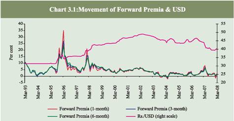
A swap transaction in the foreign exchange market is a combination
of a spot and a forward in the opposite direction. Foreign exchange
swaps account for the largest share of the total derivatives turnover in
India, followed by forwards and options. In the Indian context, the forward
price of the rupee is not essentially determined by the interest rate
differentials, but it is also significantly influenced by: (a) supply and
demand of forward US dollars; (b) interest differentials and expectations
of future interest rates; and (c) expectations of future US dollar-rupee
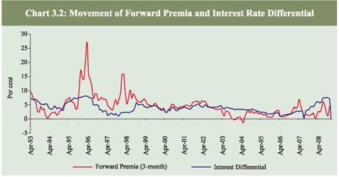
exchange rate (Chart 3.1).
Empirical studies in the Indian context reveal that forward premia
on US dollar is driven to a large extent by the interest rate differential in
the interbank market of the two economies combined with FII flows,
current account balance as well as changes in exchange rates of US dollar
vis-à-vis Indian rupee (Sharma and Mitra, 2006). Further empirical
analysis for the period January 1995-December 2006 have shown that the ability of forward rates in correctly predicting the future spot rates
has improved overtime and there is co-integration relationship between
the forward rate and the future spot rate (RCF, 2005-06).
 |
With the opening up of the capital account, the forward premia is
getting aligned with the interest rate differential reflecting market
efficiency (Chart 3.2). While free movement in capital account is only a
necessary condition for full development of forward and other foreign
exchange derivatives market, the sufficient condition is provided by a
deep and liquid money market with a well-defined yield curve in place.
Market Efficiency
With the exchange rate primarily getting determined in the market,
the issue of foreign exchange6 market efficiency has assumed importance
for India in recent years. The bid-ask spread of Rupee/US$ market has
almost converged with that of other major currencies in the international market. On some occasions, in fact, the bid-ask spread of Rupee/US$
market was lower than that of some major currencies.
 |
Besides maintaining orderly conditions, markets are perceived as efficient
when market prices reflect all available information, so that it is not possible
for any trader to earn excess profits in a systematic manner. The efficiency/
liquidity of the foreign exchange market is often gauged in terms of bid-ask
spreads. The bid-ask spread refers to the transaction costs and operating
costs involved with the transaction of the currency. These costs include phone
bills, cable charges, book-keeping expenses, trader salaries, etc. in the spot
segment, it may also include the risks involved with holding the foreign
exchange. These costs/bid-ask spread may reduce with the increase in the
volume of transaction of the currency.
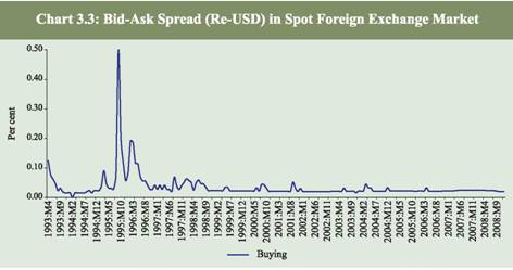
In the Indian context, it is found that the spread is almost flat and
very low. In India, the normal spot market quote has a spread of 0.25
paisa to 1 paise while swap quotes are available at 1 to 2 paise spread.
A closer look at the bid-ask spread in the rupee-US dollar spot market
reveals that during the initial phase of market development (i.e., till the mid 1990s), the spread was high and volatile due to thin market with
unidirectional behavior of market participants (Chart 3.3). In the later period,
with relatively deep and liquid markets, bid-ask spread has sharply declined
and has remained low and stable, reflecting efficiency gains.
 |
Thus, the foreign exchange market has evolved over time as a deep,
liquid and efficient market as against highly regulated market prior to
the 1990s. The market participants have become sophisticated, the range
of instruments available for trading has increased, the turnover has also
increased, while the bid-ask spreads have declined. The next Section
discusses the dynamics of capital flows, which are also key variables in
the modelling exercise.
SECTION IV
Capital Flows and Exchange Rates: The Indian Experience
The capital inflows and outflows have implications for the conduct
of domestic monetary policy and exchange rate management. The emerging market economies including India had seen a very sharp rise
in capital flows in the past few years. The surge in the capital flows till
2007-08 had coincided mostly with a faster pace of financial liberalization,
particularly a move towards regulation free open economies. Moreover,
high interest rates prevailing in the emerging market economies had led
to a wider interest rate differential in favour of the domestic markets,
which stimulated a further surge of capital flows. In emerging markets,
capital flows are often relatively more volatile and sentiment driven, not
necessarily being related to the fundamentals in these markets. Such
volatility imposes substantial risks on the market agents, which they
may not be able to sustain or manage (Committee on the Global Financial
System, BIS, 2009). In the literature, several instruments have been
prescribed for sterilization purposes. Such tools include open market
operations, tightening the access of banks at the discount window,
adjusting reserve requirements or the placement of government deposits,
using a foreign exchange swap facility, easing restrictions on capital
outflows, pre-payment of external debt and promoting investment through
absorption of capital flows for growth purposes.
1. Capital Flows: Indian Context
In the recent period, external sector developments in India have been
marked by strong capital flows, which had led to an appreciating tendency
in the exchange rate of the Indian rupee up to January 2008. The
movement of the Indian rupee is largely influenced by the capital flow
movements rather than traditional determinants like trade flows (Chart
4.1). Capital flows to India, which were earlier mainly confined to small
official concessional finance, gained momentum from the 1990s after
the initiation of economic reforms. Apart from an increase in size, capital
flows to India have undergone a compositional shift from predominantly
official and private debt flows to non-debt creating flows in the post reform
period. Private debt flows have begun to increase again in the more recent
period. Though capital flows are generally seen to be beneficial to an
economy, a large surge in flows over a short span of time in excess of the domestic absorptive capacity can, however, be a source of stress to the
economy giving rise to upward pressures on the exchange rate,
overheating of the economy, and possible asset price bubbles.
The far reaching economic reforms in India in the 1990s, witnessed
a sharp increase in capital inflows as a result of capital account
liberalisation in India and a gradual decrease in home bias in asset
allocation in advanced economies. During 1990-91, it was clear that the
country was heading for a balance of payment crisis due to deficit financed
fiscal expansion of the 1980s and the trigger of oil price spike caused by
the Gulf War. The balance of payments crisis of 1991 led to the initiation
of reform process. The broad approach to reform in the external sector
was based on the recommendations made in the Report of the High Level
Committee on Balance of Payments (Chairman: Shri. C. Rangarajan),
1991. The objectives of reform in the external sector were conditioned
by the need to correct the deficiencies that led to payment imbalances in
1991. Recognizing that an inappropriate exchange rate regime,
unsustainable current account deficit and a rise in short term debt in
relation to the official reserves were amongst the key contributing factors to the crisis, a series of reform measures were put in place. The measures
included a swift transition to a market determined exchange rate regime,
dismantling of trade restrictions, moving towards current account
convertibility and gradual opening up of the capital account. While
liberalizing the private capital inflows, the Committee recommended,
inter alia, a compositional shift in capital flows away from debt to nondebt
creating flows; strict regulation of external commercial borrowings,
especially short term debt; discouraging volatile element of flows from
non-resident Indians; and gradual liberalization of outflows.
Among the components, since the 1990s, the broad approach towards
permitting foreign direct investment has been through a dual route, i.e.,
automatic and approval, with the ambit of automatic route progressively
enlarged to almost all the sectors, coupled with higher sectoral caps
stipulated for such investments. Portfolio investments are restricted to
institutional investors. The approach to external commercial borrowings
has been one of prudence, with self imposed ceilings on approvals and a
careful monitoring of the cost of raising funds as well as their end use.
In respect of NRI deposits, some modulation of inflows is exercised
through specification of interest rate ceilings and maturity requirements.
In respect of capital outflows, the approach has been to facilitate direct
overseas investment through joint ventures and wholly owned subsidiaries
and provision of financial support to exports, especially project exports
from India. Ceilings on such outflows have been substantially liberalized
over time. The limits on remittances by domestic individuals have also
been eased. With progressive opening up of its capital account since the
early 1990s, the state of capital account in India today can be considered
as the most liberalized it has ever been in its history since the late 1950s.
All these developments have ramifications on exchange rate management
(Mohan 2008b).
2. Management of Capital Flows and Exchange Rates
The recent episode of capital flows, which has occurred in the
backdrop of current account surplus in most of the emerging Asian economies, highlights the importance of absorption of capital flows. The
absorption of capital flows is limited by the extant magnitude of the
current account deficit, which has traditionally been low in India, and
seldom above 2 per cent of GDP. In India, with a view to neutralising the
impact of excess forex flows on account of a large capital account surplus,
the central bank has intervened in the foreign exchange market at regular
intervals. But unsterilised forex market intervention can result in
inflation, loss of competitiveness and attenuation of monetary control.
The loss of monetary control could be steep if such flows are large.
Therefore, it is essential that the monetary authorities take measures to
offset the impact of such foreign exchange market intervention, partly or
wholly, so as to retain the intent of monetary policy through such
intervention.
In India, the liquidity impact of large capital inflows was traditionally
managed mainly through the repo and reverse repo auctions under the
day-to-day Liquidity Adjustment Facility (LAF). The LAF operations were
supplemented by outright open market operations (OMO), i.e. outright
sales of the government securities, to absorb liquidity on an enduring
basis. In addition to LAF and OMO, excess liquidity from the financial
system was also absorbed through the building up of surplus balances
of the Government with the Reserve Bank, particularly by raising the
notified amount of 91-day Treasury Bill auctions, forex swaps and prepayment
of external loans,
The market-based operations led to a progressive reduction in the
quantum of securities with the Reserve Bank. This apart, as per those
operations, the usage of the entire stock of securities for outright open
market sales was constrained by the allocation of a part of the securities
for day-to-day LAF operations as well as for investments of surplus
balances of the Central Government, besides investments by the State
Governments in respect of earmarked funds (CSF/GRF) while some of
the government securities were also in non-marketable lots. In the face
of large capital flows coupled with declining stock of government securities, the Reserve Bank of India introduced a new instrument of
sterilisation, viz., the Market Stabilisation Scheme (MSS) to sustain
market operations. Since its introduction in April 2004, the MSS has
served as a very useful instrument for medium term monetary and
liquidity management.
In the choice of instruments for sterilisation, it is important to
recognise the benefits from and the costs of sterilisation in general and
the relative costs/benefits in the usage of a particular instrument. The
various instruments have differential impact on the balance sheets of
the central bank, government and the financial sector. The cost of
sterilisation in India is shared by the Central Government (the cost of
MSS), Reserve Bank (sterilization under LAF) and the banking system
(in case of increase in the reserve requirements). Since surpluses of the
Reserve Bank are transferred to the Central Government, on a combined
balance sheet basis, the relative burdens of cost between the Government
and Reserve Bank are not of great relevance. However, the direct cost
borne by the Government is transparently shown in its budget accounts.
Owing to the difference between international and Indian interest rates,
there is a positive cost of sterilisation but the cost has to be traded-off
with the benefits associated with market stability, export competitiveness
and possible crisis avoidance in the external sector. Sterilized
interventions and interest rate policy are generally consistent with overall
monetary policy stance that is primarily framed on the basis of the
domestic macro-economic outlook.
With surge in capital flows to EMEs, issues relating to management
of those flows have assumed importance as they have bearings on the
exchange rates. Large capital inflows create important challenges for
policymakers because of their potential to generate overheating, loss of
competitiveness, and increased vulnerability to crisis. Reflecting these
concerns, policies in EMEs have responded to capital inflows in a variety
of ways. While some countries have allowed exchange rate to appreciate,
in many cases monetary authorities have intervened heavily in forex markets to resist currency appreciation. EMEs have sought to neutralize
the monetary impact of intervention through sterilization. Cross-country
experiences reveal that in the recent period most of the EMEs have
adopted a more flexible exchange rate regime. In view of the importance
of capital flows and foreign exchange intervention in determination of
exchange rates, these variables are included in the modelling exercise
undertaken in this study to analyze the behaviour of the exchange rate.
SECTION V
Modelling and Forecasting the Exchange Rate:
Economic Theory and Review of Literature
In the international finance literature, various theoretical models are
available to analyze exchange rate determination and behaviour. Most of
the studies on exchange rate models prior to the 1970s were based on
the fixed price assumption7. With the advent of the floating exchange
rate regime amongst major industrialized countries in the early 1970s,
an important advance was made with the development of the monetary
approach to exchange rate determination. The dominant model was the
flexible-price monetary model that has been analyzed in many early
studies like Frenkel (1976), Mussa (1976, 1979), Frenkel and Johnson
(1978), and more recently by Vitek (2005), Nwafor (2006), Molodtsova
and Papell, (2007). Following this, the sticky price or overshooting model
by Dornbusch (1976, 1980) evolved, which has been tested, amongst
others, by Alquist and Chinn (2008) and Zita and Gupta (2007). The
portfolio balance model also developed alongside8
, which allowed for
imperfect substitutability between domestic and foreign assets and
considered wealth effects of current account imbalances.
With liberalization and development of foreign exchange and assets
markets, variables such as capital flows, volatility in capital flows and forward premium have also became important in determining exchange
rates. Furthermore, with the growing development of foreign exchange
markets and a rise in the trading volume in these markets, the micro
level dynamics in foreign exchange markets increasingly became
important in determining exchange rates. Agents in the foreign exchange
market have access to private information about fundamentals or
liquidity, which is reflected in the buying/selling transactions they
undertake, that are termed as order flows (Medeiros, 2005; Bjonnes and
Rime, 2003). Microstructure theory evolved in order to capture the micro
level dynamics in the foreign exchange market (Evans and Lyons, 2001,
2005, 2007). Another variable that is important in determining exchange
rates is central bank intervention in the foreign exchange market.
Non-linear models have also been considered in the literature. Sarno
(2003), Altaville and Grauwe (2006) are some of the recent studies that
have used non-linear models of the exchange rate.
Overall, forecasting the exchange rates has remained a challenge for
both academicians as well as market participants. In fact, Meese and
Rogoff's seminal study (1983) on the forecasting performance of the
monetary models demonstrated that these failed to beat the random walk
model. This has triggered a plethora of studies that test the superiority
of theoretical and empirical models of exchange rate determination visà-
vis a random walk.
Against this backdrop, various models of exchange rate determination
are examined to derive the relevant macroeconomic fundamentals
affecting exchange rates. The empirical literature on exchange rate
determination is analyzed next.
1. Exchange Rate Models: Theoretical Considerations
(i) Theory: Purchasing Power Parity, Monetary and Portfolio Balance
Models
The earliest and simplest model of exchange rate determination,
known as the Purchasing Power Parity (PPP) theory, represented the application of ''the law of one price''. This states that arbitrage forces will
lead to the equalization of goods prices internationally once the prices
are measured in the same currency. PPP theory provided a point of
reference for the long-run exchange rate in many of the modern exchange
rate theories. It was observed initially that there were deviations from
the PPP in short-run, but in the long-run, PPP holds in equilibrium.
However, many of the recent studies like Jacobson, Lyhagen, Larsson
and Nessen (2002) find deviations from PPP even in the long-run. The reasons
for the failure of the PPP have been attributed to heterogeneity in the baskets
of goods considered for construction of price indices in various countries,
the presence of transportation cost, the imperfect competition in the goods
market, and the increase in the volume of global capital flows during the last
few decades which led to sharp deviation from PPP.
The Harrod Balassa Samuelson Model, rationalized the long run
deviations from PPP. According to this model, productivity differentials
are important in explaining exchange rates. They relax PPP assumption
and allow real exchange rates to depend on relative price of non-tradables
which are a function of productivity differentials. Chinn (1999) and
Clostermann and Schnatz (2000) find that a model with productivity
differentials, better explains and forecasts exchange rate behaviour.
The failure of PPP models gave way to Monetary Models which took
into account the possibility of capital/bond market arbitrage apart from
goods market arbitrage assumed in the PPP theory. In the monetary
models, it is the money supply in relation to money demand in both
home and foreign country, which determine the exchange rate. The
prominent monetary models include the flexible and sticky-price
monetary models of exchange rates as well as the real interest differential
model and Hooper-Morton's extension of the sticky-price model. In this
class of asset market models, domestic and foreign bonds are assumed
to be perfect substitutes.
The Flexible-Price Monetary Model (Frenkel, 1976) assumes that
prices are perfectly flexible. Consequently, changes in the nominal interest rate reflect changes in the expected inflation rate. A relative increase in
the domestic interest rate compared to the foreign interest rate implies
that the domestic currency is expected to depreciate through the effect
of inflation which causes the demand for the domestic currency to fall
relative to the foreign currency. In addition to flexible prices, the model
also assumes uncovered interest parity, continuous purchasing power
parity and the existence of stable money demand functions for the
domestic and foreign economies.
The model further implies that an increase in the domestic money
supply relative to the foreign money supply would lead to a rise in
domestic prices and depreciation of the domestic currency to maintain
PPP. Further, an increase in domestic output would lead to an appreciation
of the domestic currency since an increase in real income creates an
excess demand for domestic money supply. This, in turn, causes a
reduction in aggregate demand as agents try to increase their real money
balances leading to a fall in prices until money market equilibrium is
restored.
In the Sticky-Price Monetary Model (due originally to Dornbusch,
1976), changes in the nominal interest rate reflect changes in the tightness
of monetary policy. When the domestic interest rate rises relative to the
foreign rate, it is because there has been a contraction in the domestic
money supply relative to the domestic money demand without a matching
fall in prices. The higher interest rate at home attracts a capital inflow,
which causes the domestic currency to appreciate. This model retains
the assumption of stability of the money demand function and uncovered
interest parity but replaces instantaneous purchasing power parity with
a long-run version.
Since the PPP holds only in the long-run, an increase in the money
supply does not depreciate the exchange rate proportionately in the shortrun.
In the short-run, because of sticky prices, a monetary expansion
leads to a fall in interest rates resulting in a capital outflow. This causes
the exchange rate to depreciate instantaneously and overshoot its equilibrium level to give rise to an anticipation of appreciation in order
to satisfy the uncovered interest parity condition. The above analysis
assumes full employment so that real output is fixed. If instead, output
responds to aggregate demand, the exchange rate and interest rate
changes will be dampened.
Frankel (1979) argued that a drawback of the Dornbusch (1976)
formulation of the sticky-price monetary model was that it did not allow a
role for differences in secular rates of inflation. He develops a model that
emphasizes the role of expectation and rapid adjustment in capital markets.
The innovation is that it combines the assumption of sticky prices with that
of flexible prices with the assumption that there are secular rates of inflation.
This yields the real interest differential model.
Hooper and Morton (1982) extend the sticky price formulation by
incorporating changes in the long-run real exchange rate. The change in
the long-run exchange rate is assumed to be correlated with unanticipated
shocks to the trade balance. They therefore introduce the trade balance
in the exchange rate determination equation. A domestic (foreign) trade
balance surplus (deficit) indicates an appreciation (depreciation) of the
exchange rate.
The four models discussed above can be derived from the following
equation specified in logs with starred variables denoting foreign
counterparts:
 |
 |
These models can be further extended to incorporate portfolio choice
between domestic and foreign assets. The portfolio balance model
assumes imperfect substitutability between domestic and foreign assets.
It is a dynamic model of exchange rate determination that allows for the
interaction between the exchange rate, current account and the level of
wealth. For instance, an increase in the money supply is expected to lead
to a rise in domestic prices. The change in prices, in turn, can affect net
exports and thus imply changes in the current account of the balance of
payments. This, in turn, affects the level of wealth (via changes in the
capital account) and consequently, asset market and exchange rate
behaviour. Under freely floating exchange rates, a current account deficit
(surplus) is compensated by accommodating transactions in the capital
account i.e. capital account surplus (deficit). This has implications for
the demand and supply of currency in the foreign exchange market, which
can lead to appreciation (depreciation) of the exchange rate. Thus the
coefficient of the current account differential in the exchange rate model
is hypothesized to have a positive sign. The portfolio approach thus
introduces current account in the exchange rate equation. The theoretical
model can be expressed as a hybrid model as follows:
 |
(ii) Theory: Capital flows, forward premium
With an increase in liberalization and opening up of capital accounts
the world over, capital flows have become important in determining
exchange rate behaviour. The relation between capital flows and exchange rates is hypothesized to be negative (with the exchange rate defined as
the price of foreign currency in domestic currency). This is because capital
inflow implies purchase of domestic assets by foreigners and capital
outflow as purchase of foreign assets by residents. Since the exchange
rate is determined by the supply and demand for foreign and domestic
assets, the purchase of foreign assets drives up the price of foreign
currency. Likewise, the purchase of domestic assets drives up the price
of domestic currency. Thus, an increase in capital inflows leads to
appreciation of the domestic currency when there is no government
intervention in the foreign exchange market or if there is persistent
sterilized intervention. In the case of unsterilized government intervention,
the potential of capital inflows to influence exchange rates decreases to a
great extent.
Dua and Sen (2009) develop a model which examines the relationship
between the real exchange rate, level of capital flows, volatility of the
flows, fiscal and monetary policy indicators and the current account
surplus, and find that an increase in capital inflows and their volatility
lead to an appreciation of the exchange rate. The theoretical sign on
volatility can, however, be positive or negative.
The forward premium measured by the difference between the
forward and spot exchange rate can provide useful information about
future exchange rates. According to covered interest parity, the interest
differential between two countries equals the premium on forward
contracts. Thus, if domestic interest rates rise, the forward premium
on the foreign currency will rise and the foreign currency is expected to
appreciate. The exchange rate defined as the price of foreign currency in
domestic currency and the forward premium are therefore expected to
be positively related.
(iii) Theory: Microstructure Framework
The microstructure theory of exchange rates provides an alternative
view to the determination of exchange rates. Unlike macroeconomic
models that are based on public information, micro-based models suggest that some agents may have access to private information about
fundamentals or liquidity that can be exploited in the short-run. In
microeconomic models of asset prices, transactions play a causal role in
price determination (Evans and Lyons, 2001, 2007). The causal role
arises because transactions convey information that is not common
knowledge. These models assume that information is dispersed and
heterogeneous agents have different information sets. The trading process
in foreign exchange markets is not transparent and features bid-ask
spreads that reflect the costs to market makers / dealers of processing
orders and managing inventories. Thus, a distinctive feature of the
microstructure models is the central role played by transactions volume
or order flows in determining nominal exchange rate changes (Medeiros,
2005; Bjonnes and Rime 2003).
Order flow is the cumulative flow of transactions, signed positively
or negatively depending on whether the initiator of the transaction is
buying or selling. Order flow takes positive values if the agent purchases
foreign currency from the dealer and takes negative values if it sells at
the dealer's bid. Conventionally, order flow is taken as purchase minus
sales of foreign currency. Hence an increase in order flow (i.e. an increase
in the volume of positively signed transactions) will generate forces in
the foreign exchange market such that there is pressure on the domestic
exchange rate to depreciate. Hence the order flow and the exchange rate
are positively related. The explanatory power or information content of
order flow depends on the factors that cause it. Order flow is most
informative when it is caused due to dispersion of private information
amongst agents with respect to macroeconomic fundamentals (Evans
and Lyons, 2005). Order flow is less informative when it is caused due
to management of inventories by the foreign exchange dealers in response
to liquidity shocks.
If the dealers of foreign exchange are heterogeneous and have
different information sets, then there is information asymmetry in the
foreign exchange market. In this case, order flow will capture the
reaction of the market (obtained from aggregating the different reactions of the dealers having different information sets) to changes in
macroeconomic fundamentals and news related to changes in economic
conditions. As macroeconomic fundamentals change, future
expectations of the dealers of foreign exchange also change and so they
adjust their portfolio of foreign currency accordingly, leading to a change
in exchange rates. Another aspect of micro structure theory that has
drawn attention is the liquidity effect of order flow. Studies in the
literature have empirically tested whether the relationship between order
flow and exchange rates is due to liquidity effects that are temporary in
nature such as the herding behaviour of foreign exchange dealers
(Breedon and Vitale 2004).
(iv) Theory: Intervention
Intervention by the central bank in the foreign exchange market also
plays an important role in influencing exchange rates in countries that
have managed floating regime. With the growing importance of capital
flows in determining exchange rate movements in most emerging market
economies, intervention in foreign exchange markets by central banks
has become necessary from time to time to contain volatility in foreign
exchange markets.
The motive of central bank intervention may be to align the current
movement of exchange rates with the long-run equilibrium value of
exchange rates; to maintain export competitiveness; to reduce volatility
and to protect the currency from speculative attacks. Many studies in
the literature including Edison (1993), Dominguez and Frankel (1993),
Almenkinders (1995) and more recently Sarno and Taylor (2001) and
Neely (2005) survey the literature on modelling the reaction function of
the central bank and assessing the effectiveness of intervention.
Intervention is of two types - sterilised and non-sterilised. Intervention
is sterilised if the sale or purchase of foreign currency is accompanied
by expansionary or contractionary open market operations, so that
domestic money supply is insulated from the effects of foreign exchange
sale/purchase. Intervention is unsterilised if the sale or purchase of foreign currency is not accompanied by offsetting open market operations. The
impact of sterilised and unsterilised intervention on exchange rates can
be quite different.
In case of non-sterilised intervention, say, purchase of foreign
exchange (to prevent appreciation) not accompanied by contractionary
open market operations, money supply increases, which reduces the rate
of interest and increases demand. This leads to capital outflow on one
hand and an increase in import demand on the other. All this leads to an
increase in the demand for foreign currency and hence the exchange rate
depreciates. Thus non-sterilised intervention and exchange rates are
positively related.
While non-sterilised intervention directly influences the exchange rate
through the monetary channel, sterilised intervention also influences
exchange rate through different channels - by changing the portfolio
balance, through the signaling channel where sterilised purchase of
foreign currency will lead to a depreciation of the exchange rate if the
foreign currency purchase is assumed to signal a more expansionary
domestic monetary policy and more recently, the noise-trading channel,
according to which, a central bank can use sterilised interventions to
induce noise traders to buy or sell currency. Hence the overall effect of
sterilised intervention on exchange rates is ambiguous.
Kletzer and Kohli (2001) develop a theoretical model and discuss
the role of financial repression in exchange rate management in the Indian
context. They find that policy instruments of financial repression can be
used as tools for exchange rate intervention under managed float.
Recognizing the importance of both monetary models as well as micro
structure theory in determining the exchange rates, the study uses a
combination of both the models. Exchange rate is determined by monetary
variables as well as order flows. Theory has been further expanded to
include forward premia, capital inflows, volatility of capital flows and
central bank intervention as determining the exchange rate behaviour.
The theoretical model so generated can be expressed as follows:
2. Exchange Rate Models: Empirical Results
The previous section discusses sequentially the theoretical models
that potentially determine exchange rate behaviour. The empirical performance of these theoretical models in forecasting and explaining
exchange rate behaviour is crucial in determining the superiority of one
theory over the other. A caveat, of course, is that if a theory can explain
the behaviour of the exchange rate better than others, it does not
necessarily imply that it can also forecast exchange rates with relatively
greater accuracy, and vice versa.
Some of the empirical findings for the various theoretical frameworks
are given below. An extensive survey of literature is also available in
Dornbusch (1990), Frankel and Rose (1994), Taylor (1995), Cuthbertson
(1996), Sarno and Taylor (2002), Gandolfo (2006) and Schmidt (2006).
The main conclusions drawn from the survey of literature are summarized
as under.
(i) Empirics: Purchasing Power Parity, Monetary and Portfolio Balance
Models
Frenkel (1976) suggests that PPP holds in the long-run but not in
short-run because of price stickiness in goods market. However,
stationarity of the variables is not tested and the fact that exchange rate
and prices are endogenous is not taken into account.
Recent studies that overcome these shortcomings like Johnson
(1990), Kong (2000), Lothian and Mc Carthy (2001), Kleijn and Dijk
(2001) and Bahrumshah, Sen and Ping (2003), Diaz (2003), also find
that PPP is a long-run phenomenon. Reitz (2002) studied the performance
of PPP during periods of central bank intervention and found that PPP is
not strengthened during intervention. On the other hand, many other
studies like Jacobson, Lyhagen, Larsson and Nessen (2002), Cheung,
Chinn and Pascual (2004) find that PPP is not a common phenomenon
even in the long-run. Hence the evidence in favour of the PPP theory is
mixed. In another strand of work on modelling the exchange rate, Apte
et al. characterize the equilibrium exchange rate in a general equilibrium
economy and show that standard regressions or cointegration tests of
PPP suffer from missing variable biases and ignore variations in risk
aversion across countries and overtime.
Early studies which modelled exchange rates using the flexible price
monetary model such as Frenkel (1976), Bilson (1978), Hodrick (1978),
Putnam and Woodbury (1980), and Dornbusch (1984) support the
performance of the flexible price monetary model in modelling and
forecasting exchange rates. Subsequent studies by Frankel (1979), Driskill
and Sheffrin (1981) and Taylor (1995), however, fail to support the
performance of the flexible price monetary model and real interest
differential model in terms of explaining the exchange rate behaviour.
Empirical studies on the sticky price version of the monetary model
show mixed results and suggest weak performance in explaining exchange
rate movements. On one hand, studies like Driskill (1981) show that the
sticky price monetary model explains exchange rates well, while studies
such as Backus (1984) show that the sticky price monetary model fails
to explain the exchange rate behaviour.
Buiter and Miller (1981) proposed an extended version of the sticky
price monetary model, which included trend inflation, which was put to
test by Barr (1989) and Smith and Wickens (1986, 1990). These studies
support the extended version of the model, in terms of forecasting
exchange rates.
The empirical literature suggests that there is no consensus among
economists on the appropriate monetary model that explains exchange
rates well. It is also observed that the in-sample predictive performance
of monetary models was good in the years following the breakdown of
the Bretton Woods system (see e.g. Frankel 1976, 1979; Bilson 1978),
but their performance collapsed in the 1980s.
Meese and Rogoff (1983) recognized the limitations of testing the insample
predictive accuracy (that simply tell us that the model fits the
data reasonably well), and examined the out-of-sample predictive
performance of the monetary models vis-à-vis the simple random-walk
model. They observed that the forecasts using models based on economic
fundamentals were in all cases worse than a random walk model. In
response to this study, some of the studies tried to improve the forecasting performance of the monetary models using advanced techniques. Some
other studies gave up the monetary model and tried to improve the
forecasting performance of exchange rates using pure technical time
series techniques. There were also studies that tried to explain the
movement of the exchange rate through a suitable economy-wide
macroeconometric model capable of capturing all complex associations
between exchange rate and other variables. For example, using an
economy-wide macro econometric model for Italy, Gandolfo and Padaon
(1990) and Gandolfo (2006) have shown that an economy-wide model
beats the random walk (which in turn outperformed the traditional
structural models) in out-of-sample forecasts of the exchange rate. There
were also many studies, which investigated the reasons for the failure
of monetary models.
Meese (1990) attributed the failure of monetary models to weaknesses
in their underlying relationships such as the PPP condition, the instability
found in money demand functions and expectations that agents' forecasts
do not obey the axioms of rational expectations. Meese and Rose (1991)
observed that the non-linearity in money demand functions is not
responsible for failure of monetary models in explaining and forecasting
exchange rates. This is because the statistical performance of the
monetary model could not be improved using a non-linear money demand
function.
Flood and Rose (1995) compare the volatility in the exchange rate
and in economic fundamentals for periods of fixed and floating rates.
While exchange rates exhibit substantial volatility in the floating rate
periods, a corresponding increase in volatility was not observed in the
economic fundamentals. This led Flood and Rose to speculate that it is
unlikely that any exchange rate model based only on economic
fundamentals will prove adequate. This view is also supported by Baxter
and Stockman (1989) who further explain that there are speculative forces
in the foreign exchange market that are important in determining
exchange rates, which are not reflected in the behaviour of macroeconomic
variables.
Studies by MacDonald and Taylor (1991, 1993, 1994), Choudhary
and Lawler (1997), Diamandis, Georgoutsos and Kouretas (1998), Mark
and Sul (2001) attributed monetary models to be long-run equilibrium
phenomena. Empirical literature (e.g. Chinn and Meese, 1995; Taylor,
1995; Neely and Sarno, 2002; Sarno and Taylor, 2002) suggests that
over short horizons of one to three years, monetary fundamentals
generally do not predict changes in the spot rate. However, over longer
horizons of four to five years, fundamentals do provide predictive power
for some currencies (Kim and Mo, 1994; Mark, 1995; Chinn and Meese,
1995). These studies examine the predictive power of structural exchange
rate models using parametric and non-parametric techniques and find
that the random walk model outperforms monetary models in forecasting
exchange rates in the short-run. But in the long-run, the monetary model
outperforms the random walk model.
Some of the recent empirical studies on the monetary model
performance have also exhibited mixed results. Studies have shown that
inclusion of exchange rate expectations and the degree of openness in
the Dornbusch sticky price monetary model improves forecast ability of
the monetary model (Zita and Gupta, 2007). While models involving
Taylor-rule interest rate reaction functions forecast well when there is
exchange rate targeting, the random walk, however, remains unbeaten in
terms of forecasting ability (Molodtsova and Papell, 2007). Alquist and
Chinn (2008), however, report that structural models do not perform as
poorly as suggested by earlier studies.
Recognizing the fact that monetary models do work in the long-run,
studies have also attempted to obtain a combined forecast of all the monetary
models and compared them with the benchmark obtained by the random
walk model and the historical average return. Empirical results so obtained
suggest the superiority of combined forecasts over benchmarks and generally
yield better results than a single model (Lam et. al, 2008).
For the portfolio balance model (PBM) of exchange rate determination,
not much empirical literature is available because of data limitations, which restricts the empirical application of the portfolio balance model.
The earlier studies that estimated the log-linear version of the reduced
form portfolio balance model such as Branson, Halttunen and Masson
(1977), Bisignano and Hoover (1982) and Dooley and Isard (1982) find
dismal performance of the portfolio balance model in explaining exchange
rate behaviour. Studies by Frankel (1982a, b) and Rogoff (1984) did not
find any support in favour of the model. On the other hand, some
empirical support for the portfolio balance model is provided by Backus
(1984), Lewis (1988) and Dominguez and Frankel (1993).
(ii) Empirics: Capital Flows, Forward Premium, Central Bank
Intervention
Dua and Sen (2009) find that an increase in both net capital inflows
and their volatility lead to an appreciation of the exchange rate, and that
they jointly explain a large part of the variations in exchange rate in the
Indian economy. Kohli (2001) analyses the effect of capital flows in the
Indian context and finds that the inflow of foreign capital results in a
real appreciation of the exchange rate.
Calvo, Leiderman and Reinhart (1993) and Edwards (1999a), analyze
the impact of capital flows on the exchange rate for Latin American and
Asian countries and find that an increase in capital flows cause the
exchange rate to appreciate. However, the degree of appreciation or the
strength of the relation between capital flows and the exchange rate may
vary across countries and time.
Clarida and Taylor (1997) examine the ability of the forward exchange
rate in forecasting exchange rates and argued that failure of the forward
exchange rate in predicting future spot rates does not imply that forward
exchange rates don't contain valuable information for forecasting exchange
rates. Using the linear Vector Error Correction Model (VECM), they extract
information from the term structure of forward premia and produce outof-
sample forecasts that outperform the forecasts from the random walk
model. Clarida, Sarno, Taylor and Valente (2003) use the Markov
Switching Intercept Heteroskedastic VECM model for the term structure of forward premia and find that this model outperforms the linear VECM
and the random walk model in terms of its forecasting performance.
More recently, Della Corte, Sarno and Tsiakas, (2007) examine the
predictive ability of exchange rate models based on lagged values of the
forward premium and other macroeconomic variables, as compared to
the random walk model. The study finds that the predictive ability of
forward exchange rate premia has substantial economic value in
predicting exchange rates compared to a random walk model.
With respect to the effect of intervention, Dominguez and Frankel
(1993) examine its impact on exchange rates using primary survey data
along with secondary intervention data. They find that intervention has
a significant effect on exchange rates. Neely (2000) surveyed central
bankers who conduct intervention, and reports that intervention is
effective in changing exchange rates. Fatum and King (2005) analyse the
effects of Canadian intervention and find that intervention does
systematically affect exchange rates and is associated with reduced
volatility in exchange rates.
Other recent studies that use high frequency data (see e.g. Payne and
Vitale, 2003; Dominguez 2003a,b) form a consensus that intervention
has significant effects on exchange rates, especially in the very shortrun.
Reitz (2002) concludes that the predictive power of forecasting
methods increases in the case of intervention in the foreign exchange
market by the central bank, relative to cases when the central bank does
not intervene.
(iii) Empirics: Microstructure Theory
The micro structure theory of exchange rates gained popularity since
the late 1990s when it was empirically tested that information in order
flows drives exchange rates (Evans and Lyons, 1999; Luo, 2001; Medeiros,
2005). In a landmark study by Evans and Lyons (2001), three sources of
exchange rate variation were identified, i.e. direct effect of changes in
macro fundamentals, indirect effects of changes in macro fundamentals
via order flow and order flow not related to macro news. The use of a pseudo GARCH model with high frequency hourly data reveals that the
news of intervention increases the effect of order flow on the exchange
rate (Scalia, 2006). Recognizing that news effects are not common
knowledge and are not impounded in exchange rates directly, Evans and
Lyons (2007) have tried to quantify the effect of news on exchange rates.
They observe that two-thirds of the effect of macro news on exchange
rates is transmitted via order flow.
Bjonnes and Rime (2003) find that private information plays an
important role in the foreign exchange market and has a permanent effect
on exchange rates. Order flows carrying this private information are hence
important in determining exchange rates. Marsh and Rourke (2005) find
that order flows from profit seeking financial institutions are positively
correlated with exchange rate and flows from non-financial corporates
are negatively correlated. They also find that the impact of order flow on
exchange rate increases, as probability of flow from the informed source
increases. These views are also supported by Menkhoff and Schmeling
(2006) who find that order flows coming from centres of political and
financial decision making influence exchange rates permanently.
Mizuno, Takayasu and Takayasu (2004) find that traders in the
foreign exchange market use past information on exchange rates to carry
out transactions. This feedback of information from traders is responsible
for autocorrelation in exchange rate changes and volatility.
The survey of literature based on microstructure theory by Sager
and Taylor (2006) critically examines the role of order flows in forecasting
exchange rates. They indicate that inter-dealer order flows can explain
exchange rates contemporaneously, but cannot help to improve out-ofsample
exchange rate forecasts. This is because order flow data comes
with publication lags. These results cast doubt on the practical value of
order flow data for traders in the foreign exchange market.
Another aspect of asset market approach that has been empirically
tested is whether there are systematic and meaningful effects of
macroeconomic news on exchange rates. Love and Paynes (2002) find that the order flow is more informative around macroeconomic data
releases. Additionally, recent studies like Galati and Ho (2003) and
Andersen et. al (2003) report evidence of an asymmetric response of
exchange rates to news. Markets respond differently to positive or
negative news from the same category. This evidence once again
contradicts the proposition of the asset market theory to exchange rate
determination (Schmidt, 2006). These results indicate that the response
of traders in the foreign exchange market to macroeconomic
announcements or data releases influence exchange rates, via order flows.
(iv) Empirics: Time Series and Non-Linear Models
The general failure of structural models in explaining movements in
the spot exchange rate has led researchers to consider time series and
non-linear models. Vector Autoregression Models, Vector Error Correction
Models and Bayesian Vector Sutoregression formulations of the monetary
models of exchange rate determination for developed countries are known
to have produced forecasts which beat the random walk (see. e.g.
MacDonald and Taylor (1993, 1994) and Chaudhry and Lawler (1997)
for VAR; Chen and Leung (2003) for BVAR and BVECM; Zita and Gupta
(2007) for VAR, VECM, BVAR and BVECM). Goldberg and Frydman
(2001) maintain that the existing macroeconomic exchange rate models
are able to explain monthly or quarterly movements of exchange rates
for some sub-periods reasonably well while for others their explanatory
power completely disappears. This finding led them to suggest that
empirical exchange rate models with fixed coefficients are unlikely to
perform well either in-sample or out-of-sample. Analyzing the relationship
between exchange rates and fundamentals in a non-linear framework,
De Grauwe and Vansteenkiste (2001) also find significant switches in
the coefficients.
Sarno (2003) observes that a non-linear framework produces both
better point forecasts and measure of uncertainty surrounding the
forecasts. They further observe that the Markov Switching Intercept
Heteroscedastic (MSIH) VECM gives more accurate results than the random walk. Moreover, MSIH outperforms the linear VECM. Studies
such as Cheung, Cinn and Pascual (2004) have reported that model
specifications/currency combinations that produce accurate forecasts at
certain horizons may not do so at other horizons. Similarly, some models
or specifications may forecast certain exchange rates well, but not others.
In other words there is no unique model or specification that may forecast
well for all currencies and at all time horizons. It has also been empirically
tested that while linear models outperform at short forecast horizons,
non-linear models dominate at longer horizons (Altaville and Grauwe,
2006).
Many studies like Diebold, Gardeazabal and Yilmaz (1994), Hock
and Tan (1996), and Trapletti, Geyer and Leisch (2002) analyse the
dynamics of the foreign exchange market and see whether there is comovement
between different exchange rates. They report that observing
the trading strategy in the foreign exchange market for a particular
currency may provide additional information about the movement of
another currency and thus produce better out-of-sample forecasts.
However, their forecast performance results are not encouraging.
The common conclusion of these studies is that time series methods
can produce accurate forecasts only in the very short-run but not in the
medium or long-run. On the other hand, studies that use fractional
integration or fractional cointegration methods (e.g. Baillie and Bollerslev,
1994; Belkacem, Meddeb and Boubaker, 2005; Chortareas, Nankewis
and Jiang, 2007) support the view that different exchange rates may be
tied to each other through a long memory process, and that it is possible
to predict one exchange rate, given the observations of the other.
The literature on modelling or forecasting exchange rate volatility
uses ARCH, GARCH, FIGARCH, E-GARCH models (e.g. Martens, 2001;
Wang, Fawson, Barett and Mc Donald, 2001; Bauwens and Sucarat, 2006;
Chortareas, Nankervis and Jiang, 2007). There is a consensus that using
higher frequency data improves the forecast performance of exchange
rate volatility over that of lower frequency data.
3. Summing up: Theory and Empirics
In sum, several exchange rate models available in the literature have
been tested during the last two and a half decades. No particular model
seems to work best at all times/horizons. Monetary models based on the
idea of fundamental driven exchange rate behaviour work best in the
long-run, but lose their predictability in the short-run to naïve random
walk forecasts. The volatility of exchange rates also substantially exceeds
that of the volatility of macro economic fundamentals, thus providing
further evidence of weakening fundamental-exchange rate link. A
combination of the different monetary models, however, at times gives
better results than the random walk. Order flows also play an important
role in influencing the exchange rate. Keeping in view all the above results
of the literature, this study attempts to develop a model for the rupeedollar
exchange rate taking into account all the different monetary models
along with the microstructure models incorporating order flow, as well
as capital flows, forward premium and central bank intervention.
SECTION VI
Modelling and Forecasting the Exchange Rate:
Econometric Methodology
This study employs Vector Autoregressive (VAR) and Bayesian Vector
Autoregressive (BVAR) models to estimate the monetary model of the
exchange rate (Re/$) and its augmented variants. Tests for nonstationarity
are first conducted followed by tests for cointegration and Granger
causality. Finally, the VAR and BVAR models are estimated and tested
for out-of-sample forecast accuracy. This section briefly describes the
tests for nonstationarity, VAR and BVAR modelling, cointegration and
Granger causality and tests for out-of-sample forecast accuracy.
1. Tests for Nonstationarity
The classical regression model requires that the dependent and
independent variables in a regression be stationary in order to avoid the problem of what Granger and Newbold (1974) called 'spurious regression'
characterized by a high R2 , significant t-statistics but results that are
without economic meaning. A stationary series exhibits mean reversion,
has a finite, time invariant variance and a finite covariance between two
values that depends only on their distance apart in time, not on their
absolute location in time. If the characteristics of the stochastic process
that generated a time series change overtime, i.e. if the series is
nonstationary, it becomes difficult to represent it over past and future
intervals of time by a simple algebraic model. Thus the first econometric
exercise is to test if all the series are nonstationary or have a unit root.
A battery of unit root tests now exists to discern whether a time series
exhibits I(1) (unit root) or I(0) (stationary) behaviour. In this study, we employ
the augmented Dickey-Fuller (ADF) test (1979, 1981) and its more powerful
variant, the Dickey-Fuller Generalized Least Squares (DF-GLS) test proposed
by Elliot, Rothenberg and Stock (1996). These two tests share the same null
hypothesis of a unit root. An alternative test is that proposed by Kwiatkowski
et al. (1992) which has a null hypothesis of stationarity. If two of these three
tests indicate nonstationarity for any series, we conclude that the series has
a unit root. The KPSS test is also often used in conjunction with these tests
to investigate the possibility that a series is fractionally integrated (that is,
neither I(1) nor I(0)) although this is not explored in this study.
To test if a sequence yt contains a unit root using the ADF procedure,
three different regression equations are considered.
The most general form of the D-F test (equation 1) allows for both a
drift term and a deterministic trend; the second excludes the deterministic
trend; and the third does not contain an intercept or a trend term. In all
three equations, the parameter of interest is . If γ=0, the yt sequence has
unit root. The null is therefore γ=0 against the alternative γ≠0. The
estimated t-statistic is compared with the appropriate critical value in
the Dickey-Fuller tables to determine if the null hypothesis is valid. The
critical values are denoted by ττ , τμ and τ for equations (1), (2) and (3)
respectively. The D-F test presumes the existence of white noise errors
in the regression, hence lags of the dependent variable are added to the
regressions to whiten the errors.
Following Doldado, Jenkinson and Sosvilla-Rivero (1990), a
sequential procedure is used to test for the presence of a unit root when
the form of the data-generating process is unknown. This involves testing
the most general model (equation 1) first and following various tests,
moving to the most parsimonious model (equation 3). Such a procedure
is necessary since including the intercept and trend term reduces the
degrees of freedom and the power of the test implying that we may
conclude that a unit root is present when, in fact, this is not true. Further,
additional regressors increase the absolute value of the critical value
making it harder to reject the null hypothesis. On the other hand,
inappropriately omitting the deterministic terms can cause the power of
the test to go to zero (Campbell and Perron, 1991).
Compared to the ADF test, the DF-GLS test has substantially
improved power when an unknown mean or trend is present (Elliot et
al., 1996). The DF-GLS procedure relies on demeaning and/or detrending
a series prior to the implementation of the auxiliary ADF regression as
follows:
2. VAR and BVAR Modelling
In this study, we employ multivariate forecasting models in the Vector Autoregressive (VAR) and Bayesian VAR framework. A Vector Autoregressive (VAR) model does not require specification of the projected values of the exogenous variables as in a simultaneous equations model. It uses regularities in the historical data on the forecasted variables. Economic theory only selects the economic variables to include in the model. An unrestricted VAR model (Sims 1980) is written as follows:
The model uses the same lag length for all variables. A serious drawback of the VAR model, however, is that overparameterisation produces multicollinearity and loss of degrees of freedom that can lead to inefficient estimates and large out-of-sample forecasting errors. A possible solution is to exclude insignificant variables and/or lags based on statistical tests.
An alternative approach to overcome over-parameterisation uses a Bayesian VAR model as described in Litterman (1981, 1982), Doan, Litterman and Sims (1984), Todd (1984), Litterman (1986), and Spencer (1993). Instead of eliminating longer lags and/or less important variables, the Bayesian technique imposes restrictions on these coefficients on the assumption that these are more likely to be near zero than the coefficients on shorter lags and/or more important variables. If, however, strong effects do occur from longer lags and/or less important variables, the data can override this assumption. Thus, the Bayesian model imposes prior beliefs on the relationships between different variables as well as between own lags of a particular variable. If these beliefs (restrictions) are appropriate, the forecasting ability of the model should improve. The Bayesian approach to forecasting therefore provides a scientific way of imposing prior or judgmental beliefs on a statistical model. Several prior beliefs can be imposed so that the set of beliefs that produces the best forecasts is selected for making forecasts. The selection of the Bayesian prior, of course, depends on the expertise of the forecaster.
The restrictions on the coefficients specify normal prior distributions with means zero and small standard deviations for all coefficients with decreasing standard deviations on increasing lags, except for the coefficient on the first own lag of a variable that is given a mean of unity. This so-called ';Minnesota prior'; was developed at the Federal Reserve Bank of Minneapolis and the University of Minnesota.
The standard deviation of the prior distribution for lag m of variable j in equation i for all i, j, and m -- S(i, j, m) can be expressed as function of a small number of hyperparameters: w, d, and a weighting matrix
f(i,j). This allows the forecaster to specify individual prior variances for
a large number of coefficients based on only a few hyperparameters. The
standard deviation is specified as follows:
The term si equals the standard error of a univariate autoregression
for variable i. The ratio si /sj scales the variables to account for differences
in units of measurement and allows the specification of the prior without
consideration of the magnitudes of the variables. The parameter w
measures the standard deviation on the first own lag and describes the
overall tightness of the prior. The tightness on lag m relative to lag 1
equals the function g(m), assumed to have a harmonic shape with decay
factor d. The tightness of variable j relative to variable i in equation i
equals the function f(i, j). Examples of selection of hyperparameters are
given in Dua and Ray (1995), Dua and Smyth (1995), Dua and Miller
(1996) and Dua, Miller and Smyth (1999); Dua, Raje and Sahoo (2003,
2008).
The BVAR method uses Theil's (1971) mixed estimation technique
that supplements data with prior information on the distributions of the
coefficients. With each restriction, the number of observations and degrees
of freedom artificially increase by one. Thus, the loss of degrees of freedom
due to overparameterisation does not affect the BVAR model as severely.
Another advantage of the BVAR model is that empirical evidence on
comparative out-of-sample forecasting performance generally shows that
the BVAR model outperforms the unrestricted VAR model. A few examples
are Holden and Broomhead (1990), Artis and Zhang (1990), Dua and
Ray (1995), Dua and Miller (1996), Dua, Miller and Smyth (1999), Dua
and Miller (2006), Dua, Raje and Sahoo (2003, 2008).
The above description of the BVAR models assumes that the variables
are stationary. If the variables are nonstationary, they can continue to be
specified in levels in a BVAR model because as pointed out by Sims et. al
(1990, p.136) '……the Bayesian approach is entirely based on the
likelihood function, which has the same Gaussian shape regardless of
the presence of nonstationarity, [hence] Bayesian inference need take no
special account of nonstationarity'. Furthermore, Dua and Ray (1995)
show that the Minnesota prior is appropriate even when the variables
are cointegrated.
In the case of a VAR, Sims (1980) and others, e.g. Doan (1992),
recommend estimating the VAR in levels even if the variables contain a
unit root. The argument against differencing is that it discards information
relating to comovements between the variables such as cointegrating
relationships. The standard practice in the presence of a cointegrating
relationship between the variables in a VAR is to estimate the VAR in
levels or to estimate its error correction representation, the vector error
correction model, VECM. If the variables are nonstationary but not
cointegrated, the VAR can be estimated in first differences.
3. Cointegration and Granger Causality
The possibility of a cointegrating relationship between the variables
is tested using the Johansen and Juselius (1990, 92) methodology. Since
the Johansen procedure is well known in the time series literature, a
detailed explanation is not presented here.
If the presence of cointegration is established, the concept of Granger
causality can also be tested in the VECM framework. For example, if
two variables are cointegrated, i.e. they have a common stochastic trend,
causality in the Granger (temporal) sense must exist in at least one
direction (Granger, 1986; 1988). Since Granger causality is also a test
of whether one variable can improve the forecasting performance of
another, it is important to test for it to evaluate the predictive ability of
a model.
Granger-causality with respect to a particular variable can be tested
by a joint test of statistical significance of the lagged error correction
term and the lags of that explanatory variable.
4. Evaluation of Forecasting Models
Evaluation of the forecasting models is based on RMSE, Theil's U
(Theil, 1966), and the Diebold-Mariano (1995) test. The models are
initially estimated using monthly data over the period July 1996 to
December 2006 and tested for out-of-sample forecast accuracy from
January 2007 to June 2008. Recursive forecasts are generated from onethrough
twelve-months-ahead and out-of-sample forecast accuracy of
monetary model and its augmented variants is assessed. The overall
average of the U statistic and the RMSE for up to twelve-months-ahead
is also calculated to gauge the accuracy of a model.
The forecast accuracy of the VAR technique vs the BVAR method is also
evaluated.
A comparison with the naïve model is, therefore, implicit in the U-statistic.
A U-statistic of 1 indicates that the model forecasts match the performance
of naïve, no-change forecasts. A U-statistic >1 shows that the naïve forecasts outperform the model forecasts. If U is <1, the forecasts from
the model outperform the naïve forecasts. The U-statistic is, therefore, a
relative measure of accuracy and is unit-free.
Since the U-statistic is a relative measure, it is affected by the accuracy
of the naïve forecasts. Extremely inaccurate naïve forecasts can yield
U<1, falsely implying that the model forecasts are accurate. This problem
is especially applicable to series with trend. The RMSE, therefore,
provides a check on the U-statistic and is also reported.
5. Summary of Steps in Econometric Estimation
In sum, the study proceeds as follows. First, the series are tested for the presence of a unit root using the augmented Dickey-Fuller, DF-GLS and KPSS tests.
Second, multivariate models (Models 2 through 4) described in the previous section on theoretical models are estimated using the VAR and BVAR techniques. Since Model 2 is the monetary model, Models 3 and 4 examine if the forecast performance of the monetary model can be improved by including additional variables. To estimate VAR models, if all the variables are nonstationary and integrated of the same order, the Johansen test is conducted for the presence of cointegration. If a cointegrating relationship exists, the VAR model can be estimated in levels.
Tests for Granger causality are also conducted in the VECM framework to evaluate the forecasting ability of the model. Lastly, Bayesian vector autoregressive models are estimated that impose prior beliefs on the relationships between different variables as well as between own lags of a particular variable. If these beliefs (restrictions) are appropriate, the forecasting ability of the model should improve. Thus, the performance of the VAR models against the corresponding BVAR versions is also assessed.
SECTION VII
Estimation and Evaluation of Alternative Forecasting Models
The models discussed in the earlier Sections have been estimated
and evaluated in this Section. The alternative models are estimated from
July 1996 through December 2006. The out-of-sample forecasting
performance of the alternative models is evaluated over January 2007 to
June 2008 and also over the sub-period January 2007 to January 2008
to take into account the turning point in January 2008. Figure 1 shows
the movements in the Re/$ rate in the period under study: July 1996 through June 2008. Table 7.1 reports the summary statistics of the
exchange rate over the full period and the sub-periods. These statistics,
along with the plot indicate turning points in May 2002 (maximum of
Rs. 49/$), January 2007 (maximum of Rs. 44.33/$), and January 2008
(minimum of Rs. 39.37).
 |
Table 7.1: Summary Statistics for Exchange Rate |
Time Period |
Mean |
Maximum |
Minimum |
Standard
Deviation |
Jul 1996 - Jun 2008 |
43.52 |
49.00 |
35.51 |
3.73 |
|
|
(May 2002) |
(Jul 1996) |
|
Jul 1996 - Dec 2006 |
43.86 |
49.00 |
35.51 |
3.82 |
|
|
(May 2002) |
(Jul 1996) |
|
Jan 2007 – Jun 2008 |
41.12 |
44.33 |
39.37 |
1.69 |
|
|
(Jan 2007) |
(Jan 2008) |
|
Jan 2007 - Jan 2008 |
41.20 |
44.33 |
39.37 |
1.86 |
|
|
(Jan 2007) |
(Jan 2008) |
|
Feb 2008 - Jun 2008 |
40.90 |
42.82 |
39.73 |
1.28 |
|
|
(Jun 2008) |
(Feb 2008) |
|
The various models estimated in the VAR and BVAR framework are
described in Section 5 and are summarized below:
1. Theoretical Models
Model 3
9 : Model 2 + other variables (inflation differential + trade balance
differential + forward premium + capital inflows + volatility of capital
inflows + order flow)
Data definitions and sources are given in Annexure 1. Unit root tests
are conducted on the above variables. Tests for the existence of a cointegrating relationship as well for Granger causality are also
undertaken for the multivariate models given above. The models are then
estimated in the VAR and BVAR framework.
2. Tests for Nonstationarity
The first step in the estimation of the alternative models is to test for
nonstationarity. Three alternative tests are used, i.e., the augmented Dickey-
Fuller (ADF) test, the Dickey-Fuller Generalized Least Squares test and the
KPSS test. If at least two of the three tests show the existence of a unit root,
the series is considered as nonstationary. The tests for nonstationarity are
reported monthly data from June 1996 to December 2006.
Table 7.2 reports the three tests with constant and trend. The
inference at the 5% significance level is given in Table 7.3. This shows
that apart from order flow and intervention, all other variables are
nonstationary. Testing for differences of each variable confirms that all
the variables are integrated of order one.
Table 7.2: ADF, DF-GLS and KPSS Tests (Constant and trend) July 1996 to December 2006 |
VARIABLE |
ADF |
DF-GLS |
KPSS (l=8) |
1 |
2 |
3 |
4 |
et |
-1.1192 |
-0.4147 |
0.346 |
it-it* |
-2.5144 |
-2.2992 |
0.227 |
yt-yt* |
-3.0568 |
-0.5383 |
0.317 |
mt-mt* |
-0.77086 |
-0.2207 |
0.354 |
πt-πt* |
-2.6037 |
-2.9580 |
0.116 |
tb-tb* |
-2.5620 |
-3.1571 |
0.108 |
Fdpmt |
-2.6281 |
-3.3942 |
0.054 |
Volt |
-3.1237 |
-0.7189 |
0.239 |
Δoft |
-2.5657 |
-8.0816 |
0.107 |
Intt |
-24.184 |
-8.6548 |
0.122 |
Critical Value |
10% |
-3.13 |
-3.55 |
0.119 |
5% |
-3.41 |
-3.01 |
0.146 |
1% |
-3.96 |
-2.72 |
0.216 |
Table 7.3: Unit Root Test Summary July 1996 to December 2006 |
Variables |
ADF |
DF-GLS |
KPSS |
Inference |
1 |
2 |
3 |
4 |
5 |
et |
I(1) |
I(1) |
I(1) |
I(1) |
it-it* |
I(1) |
I(1) |
I(1) |
I(1) |
yt-yt* |
I(1) |
I(1) |
I(1) |
I(1) |
mt-mt* |
I(1) |
I(1) |
I(1) |
I(1) |
πt-πt* |
I(1) |
I(1) |
I(0) |
I(1) |
tb-tb* |
I(1) |
I(1) |
I(0) |
I(1) |
fdpmt |
I(1) |
I(1) |
I(0) |
I(1) |
volt |
I(1) |
I(1) |
I(1) |
I(1) |
Δoft |
I(1) |
I(0) |
I(0) |
I(0) |
intt |
I(0) |
I(0) |
I(0) |
I(0) |
a. Null hypothesis of unit root not rejected at 1%
b. Null hypothesis of no unit root not rejected at 1% but rejected at 5%.
This does not affect overall inference |
3. Tests for Cointegration and Granger Causality
Various specifications of the theoretical Model 3 were estimated using
the cointegration approach. The final model was selected based on diagnostic
checking and signs of the coefficients. The empirical models selected are
given below and their cointegration equations are reported in Table 7.4.
Empirical Models (based on overall fit)
Table 7.4: Cointegrating Equations (Dependent Variable: et)July 1996 to December 2006 |
Variable |
Model 2 |
Model 3 |
Model 4 |
1 |
2 |
3 |
4 |
it-it* |
-0.097 |
-0.126 |
-0.185 |
yt-yt* |
-1.061 |
-3.277 |
-4.228 |
mt-mt* |
2.283 |
5.585 |
6.401 |
fdpmt |
- |
0.070 |
0.0833 |
volt |
- |
-2.102 |
-1.999 |
Models 1 and 2 above are the same as the theoretical versions. Model
3 has fewer independent variables compared to its theoretical
counterpart. This directly feeds into Model 4 . Since the order flow and
intervention variables are stationary, their sign and significance is
determined in the framework of an error correction model. The empirical
signs of all the variables conform to economic theory and are given below :
The Granger causality tests for Models 2-4 are reported in Tables
7.5 -7.7 . Apart from the intervention variable, all other variables Granger
cause the exchange rate10 . This result thus justifies the inclusion of all the variables that Granger cause the exchange rate since these variables
can potentially improve the predictive performance of the model.
Models 2 through 4 are estimated both in the VAR and BVAR
frameworks and their predictive ability is evaluated over two out-of sample
periods taking into account the turning point in January 2008:
January 2007 through January 2008 and January 2007 through June
2008.
Table 7.5: Granger Causality Tests (July 1996 to December 2006) |
MODEL 2 : et= f((it-it*), (yt-yt*), (mt-mt*) |
Null Hypothesis |
Number of Lags |
χ2 [p-value] |
Conclusion |
1 |
2 |
3 |
4 |
et is not Granger caused by it-it* |
2 |
4.2082[.122] |
Reject H0 |
et is not Granger caused by yt –yt* |
2 |
6.6321[.036] |
Reject H0 |
et is not Granger caused by mt-mt* |
2 |
5.2722[.072] |
Reject H0 |
Table 7.6: Granger Causality Tests (July 1996 to December 2006) |
MODEL 3 : et = f((it-it*), (yt-yt*), (mt-mt*), fdpmt, volt, ∆oft) |
Null Hypothesis |
Number of Lags |
χ2 [p -value] |
Conclusion |
1 |
2 |
3 |
4 |
et is not Granger caused by it-it* |
2 |
4.8623[.088] |
Reject H0 |
et is not Granger caused by yt -yt * |
2 |
5.9908[.050] |
Reject H0 |
et is not Granger caused by mt -mt * |
2 |
6.1741[.046] |
Reject H0 |
et is not Granger caused by fdpmt |
2 |
4.8883[.087] |
Reject H0 |
et is not Granger caused by volt |
2 |
5.7506[.056] |
Reject H0 |
et is not Granger caused by ∆oft |
2 |
2.5585[.012]* |
Reject H0 |
* t-statistic is from the error correction model where ∆oft has a positive sign. |
Table 7.7: Granger Causality Tests (July 1996 to December 2006) |
MODEL 4 : et = f((it-it*), (yt-yt*), (mt-mt*), fdpmt, volt, ∆oft, ∆int) |
Null Hypothesis |
Number of Lags |
χ2 [p-value] |
Conclusion |
1 |
2 |
3 |
4 |
et is not Granger caused by it -it * |
2 |
5.2473[.073] |
Reject H0 |
et is not Granger caused by yt -yt * |
2 |
6.4220[.040] |
Reject H0 |
et is not Granger caused by mt -mt * |
2 |
6.5762[.037] |
Reject H0 |
et is not Granger caused by fdpmt |
2 |
5.2624[.072] |
Reject H0 |
et is not Granger caused by volt |
2 |
6.1058[.047] |
Reject H0 |
et is not Granger caused by ∆oft |
2 |
2.4236[.017]** |
Reject H0 |
et is not Granger Caused by ∆intt |
2 |
0.48722[.627]** |
Do not reject H0 |
** t-statistic from the error correction model where ∆intt has a positive sign. |
4. Empirical Results: Out-of-sample Forecasts - January 2007 to
January 2008
(i) VAR Models: January 2007 to January 2008
The forecast accuracy results for the VAR models are reported in
Table 7.8. Table 7.9 gives the Diebold-Mariano test across various VAR
models. The main results are summarized below:
a. Model 2 performs consistently better than Model 1. This implies
that the monetary model outperforms the random walk model.
b. Model 3′ performs better than Model 2 for longer term forecasts.
Thus, forecast accuracy can be improved by extending the monetary
model to include forward premium, volatility of capital inflows and
order flow.
c. Model 4′ performs better than Model 3 for longer term forecasts.
Information on intervention by the central bank thus helps to improve
forecasts at the longer end.
Table 7.8: VAR Models Out-of-sample Forecast Accuracy: January 2007 to January 2008 |
Months ahead |
No of Obs |
RMSE |
Theil U2 |
Model 1
3-mth avg |
Model 2
3-mth avg |
Model 3’
3-mth avg |
Model 4
3-mth avg |
Model 2
3-mth avg |
Model 3’
3-mth avg |
Model 4’
3-mth avg |
1 |
2 |
3 |
4 |
5 |
6 |
7 |
8 |
9 |
10 |
11 |
12 |
13 |
14 |
15 |
16 |
1 |
13 |
0.722 |
|
0.508 |
|
0.447 |
|
0.446 |
|
0.704 |
|
0.619 |
|
0.618 |
|
2 |
12 |
1.275 |
|
0.945 |
|
0.877 |
|
0.877 |
|
0.741 |
|
0.688 |
|
0.688 |
|
3 |
11 |
1.756 |
1.251 |
1.344 |
0.932 |
1.325 |
0.883 |
1.318 |
0.880 |
0.765 |
0.737 |
0.754 |
0.687 |
0.751 |
0.685 |
4 |
10 |
2.252 |
|
1.694 |
|
1.719 |
|
1.712 |
|
0.752 |
|
0.763 |
|
0.760 |
|
5 |
9 |
2.617 |
|
1.919 |
|
1.940 |
|
1.931 |
|
0.733 |
|
0.741 |
|
0.738 |
|
6 |
8 |
2.888 |
2.586 |
2.017 |
1.876 |
1.931 |
1.863 |
1.909 |
1.851 |
0.698 |
0.728 |
0.669 |
0.724 |
0.661 |
0.720 |
7 |
7 |
3.302 |
|
2.189 |
|
1.900 |
|
1.870 |
|
0.663 |
|
0.576 |
|
0.566 |
|
8 |
6 |
3.709 |
|
2.444 |
|
2.069 |
|
2.001 |
|
0.659 |
|
0.558 |
|
0.539 |
|
9 |
5 |
4.307 |
3.773 |
2.910 |
2.514 |
2.566 |
2.178 |
2.472 |
2.114 |
0.676 |
0.666 |
0.596 |
0.576 |
0.574 |
0.560 |
10 |
4 |
4.852 |
|
3.407 |
|
3.242 |
|
3.132 |
|
0.702 |
|
0.668 |
|
0.645 |
|
11 |
3 |
4.962 |
|
3.765 |
|
3.784 |
|
3.654 |
|
0.759 |
|
0.763 |
|
0.736 |
|
12 |
2 |
5.079 |
4.964 |
3.657 |
3.609 |
3.803 |
3.610 |
3.746 |
3.511 |
0.720 |
0.727 |
0.749 |
0.727 |
0.738 |
0.706 |
Average |
3.143 |
|
2.233 |
|
2.134 |
|
2.089 |
|
0.714 |
|
0.679 |
|
0.668 |
|
Note : 1. Accuracy measures are calculated using antilog of forecast and actual values although the models
are estimated using logs
2. For Model 1 (naïve forecast), Theil U2, by definition, equals one.
3. Optimal number of lags for all VAR models is 2. |
Table 7.9: DM Test for VAR Models Out-of-sample Forecast Accuracy: January 2007 to January 2008 |
Month Ahead |
Model 1 vs Model 2 |
Model 2 vs Model 3’ |
Model 3’ vs Model 4’ |
1 |
2 |
3 |
4 |
1 |
2 is better than 1b |
3 is better than 2c |
4 is better than 3c |
2 |
2 is better than 1b |
Indifferent |
Indifferent |
3 |
2 is better than 1b |
Indifferent |
Indifferent |
4 |
2 is better than 1a |
Indifferent |
Indifferent |
5 |
2 is better than 1a |
Indifferent |
Indifferent |
6 |
2 is better than 1a |
Indifferent |
Indifferent |
7 |
2 is better than 1a |
3 is better than 2c |
Indifferent |
8 |
2 is better than 1a |
3 is better than 2a |
4 is better than 3d |
9 |
2 is better than 1a |
3 is better than 2a |
4 is better than 3c |
10 |
2 is better than 1a |
3 is better than 2e |
4 is better than 3c |
11 |
2 is better than 1a |
Indifferent |
4 is better than 3a |
12 |
2 is better than 1a |
2 is better than 3 a |
4 is better than 3d |
Note : 1. “Better” implies “yields more accurate forecasts”.
2. a : significant at 1%; b : significant at 5%; c : significant at 10%; d : significant at 15%;
e : significant at 20% |
(ii) BVAR Models: January 2007 to January 2008
The forecast accuracy statistics for the BVAR models are reported in
Table 7.10. The comparison of out-of-sample forecast accuracy across
BVAR models is reported in Table 7.11. Overall, the results are generally
similar to those obtained for VAR models.
a. Model 2 (monetary model) performs consistently better than Model
1 (random walk).
b. Model 3′ performs consistently better than Model 2. In the case of VAR
models, the superiority of Model 3′ was established in the longer term
forecasts whereas in the BVAR case, this is true of all forecast horizons.
c. Model 4′ performs better than Model 3′ for longer term forecasts
implying that information on central bank intervention produces
more accurate forecasts at the longer end.
Table 7.10 : BVAR Models Out-of-sample Forecast Accuracy: January 2007 to January 2008 |
Months ahead |
No of Obs |
RMSE |
Theil U2 |
Model 1
3-mth avg |
Model 2
3-mth avg |
Model 3’
3-mth avg |
Model 4
3-mth avg |
Model 2
3-mth avg |
Model 3’
3-mth avg |
Model 4’
3-mth avg |
1 |
2 |
3 |
4 |
5 |
6 |
7 |
8 |
9 |
10 |
11 |
12 |
13 |
14 |
15 |
16 |
1 |
13 |
0.722 |
|
0.508 |
|
0.447 |
|
0.446 |
|
0.704 |
|
0.619 |
|
0.618 |
|
2 |
12 |
1.275 |
|
0.945 |
|
0.877 |
|
0.877 |
|
0.741 |
|
0.688 |
|
0.688 |
|
3 |
11 |
1.756 |
1.251 |
1.344 |
0.932 |
1.325 |
0.883 |
1.318 |
0.880 |
0.765 |
0.737 |
0.754 |
0.687 |
0.751 |
0.685 |
4 |
10 |
2.252 |
|
1.694 |
|
1.719 |
|
1.712 |
|
0.752 |
|
0.763 |
|
0.760 |
|
5 |
9 |
2.617 |
|
1.919 |
|
1.940 |
|
1.931 |
|
0.733 |
|
0.741 |
|
0.738 |
|
6 |
8 |
2.888 |
2.586 |
2.017 |
1.876 |
1.931 |
1.863 |
1.909 |
1.851 |
0.698 |
0.728 |
0.669 |
0.724 |
0.661 |
0.720 |
7 |
7 |
3.302 |
|
2.189 |
|
1.900 |
|
1.870 |
|
0.663 |
|
0.576 |
|
0.566 |
|
8 |
6 |
3.709 |
|
2.444 |
|
2.069 |
|
2.001 |
|
0.659 |
|
0.558 |
|
0.539 |
|
9 |
5 |
4.307 |
3.773 |
2.910 |
2.514 |
2.566 |
2.178 |
2.472 |
2.114 |
0.676 |
0.666 |
0.596 |
0.576 |
0.574 |
0.560 |
10 |
4 |
4.852 |
|
3.407 |
|
3.242 |
|
3.132 |
|
0.702 |
|
0.668 |
|
0.645 |
|
11 |
3 |
4.962 |
|
3.765 |
|
3.784 |
|
3.654 |
|
0.759 |
|
0.763 |
|
0.736 |
|
12 |
2 |
5.079 |
4.964 |
3.657 |
3.609 |
3.803 |
3.610 |
3.746 |
3.511 |
0.720 |
0.727 |
0.749 |
0.727 |
0.738 |
0.706 |
Average |
3.143 |
|
2.233 |
|
2.134 |
|
2.089 |
|
0.714 |
|
0.679 |
|
0.668 |
|
Note : 1. Accuracy measures are calculated using antilog of forecast and actual values although the models
are estimated using logs
2. For Model 1 (naïve forecast), Theil U2, by definition, equals one.
3. Optimal hyperparameters for all BVAR models are as follows: w=.2, d=1, k=.7
4. Optimal number of lags is 3 for Model 2 and 2 for Models 3 and 4 |
Table 7.11: DM Test for BVAR Models Out-of-sample Forecast Accuracy: January 2007 to January 2008 |
Month Ahead |
Model 1 vs Model 2 |
Model 2 vs Model 3’ |
Model 3’ vs Model 4’ |
1 |
2 |
3 |
4 |
1 |
2 is better than 1b |
3 is better than 2a |
4 is better than 3b |
2 |
2 is better than 1b |
3 is better than 2b |
Indifferent |
3 |
2 is better than 1b |
3 is better than 2a |
Indifferent |
4 |
2 is better than 1a |
3 is better than 2b |
Indifferent |
5 |
2 is better than 1a |
3 is better than 2b |
Indifferent |
6 |
2 is better than 1a |
3 is better than 2a |
Indifferent |
7 |
2 is better than 1a |
3 is better than 2b |
4 is better than 3e |
8 |
2 is better than 1a |
3 is better than 2a |
4 is better than 3c |
9 |
2 is better than 1a |
3 is better than 2a |
4 is better than 3c |
10 |
2 is better than 1a |
3 is better than 2a |
4 is better than 3c |
11 |
2 is better than 1a |
3 is better than 2a |
4 is better than 3b |
12 |
2 is better than 1a |
3 is better than 2a |
4 is better than 3e |
Note : 1. “Better” implies “yields more accurate forecasts”.
2. a : significant at 1% ; b : significant at 5%; c : significant at 10%; d : significant at 15%; e : significant at 20% |
(iii) VAR vs BVAR Models: January 2007 to January 2008
The Diebold Mariano test results for the comparison of VAR and
BVAR models for Models 3 and 4 are reported in Table 7.12.
a. BVAR Model 3′ performs almost consistently better than the
corresponding VAR model.
b. BVAR Model 4′ performs almost consistently better than the
corresponding VAR model.
The above results show that BVAR models yield more accurate forecasts
than the VAR models.
Table 7.12: DM Test for VAR vs BVAR Models Out-of-sample Period: January 2007 to January 2008 |
Model 3’ |
Model 4’ |
Month Ahead |
VAR vs BVAR |
Month Ahead |
VAR vs BVAR |
1 |
2 |
1 |
2 |
1 |
VAR better than BVARb |
1 |
VAR better than BVARb |
2 |
Indifferent |
2 |
Indifferent |
3 |
BVAR better than VARc |
3 |
BVAR better than VARc |
4 |
BVAR better than VARb |
4 |
BVAR better than VARb |
5 |
BVAR better than VARa |
5 |
BVAR better than VARa |
6 |
BVAR better than VARa |
6 |
BVAR better than VARa |
7 |
BVAR better than VARa |
7 |
BVAR better than VARa |
8 |
BVAR better than VARa |
8 |
BVAR better than VARb |
9 |
BVAR better than VARa |
9 |
BVAR better than VARb |
10 |
BVAR better than VARa |
10 |
BVAR better than VARa |
11 |
BVAR better than VARa |
11 |
BVAR better than VARa |
12 |
BVAR better than VARa |
12 |
BVAR better than VARa |
Note : 1. “Better” implies “yields more accurate forecasts”.
2. a : significant at 1% ; b : significant at 5%; c : significant at 10%; d : significant
at 15%; e : significant at 20% |
(iv) Conclusions: January 2007 to January 2008
a. The monetary model outperforms the naïve forecast model.
b. Information on the forward premium, volatility of capital inflows
and order flows improve the accuracy of forecasts. It is thus possible
to beat the monetary model.
c. Including data on central bank intervention (Model 4′) helps to
improve forecast accuracy further.
d. BVAR models yield more accurate forecasts than their VAR
counterparts.
5. Empirical Results: Out-of-sample Forecasts - January 2007 to
June 2008
(i) VAR vs BVAR Models: January 2007 to June 2008
The out-of-sample forecast accuracy statistics for the VAR model are
reported in Table 7.13 and the Diebold-Mariana test inferences for
comparison across the VAR models are given in Table 7.14. The
corresponding tables for the BVAR models are 7.15 and 7.16.
This period includes a turning point in January 2008. Possibly due
to this, the empirical results are not as sharp as those obtained in the
shorter period. At certain forecast horizons, the monetary model is not
able to beat the random walk although the extended model (Model 3′) is
almost consistently better than the monetary model for the VAR model.
The results are similar for BVAR models although the result that Model
3 produces better forecasts than Model 2 comes out more clearly in the
BVAR case. Furthermore, a comparison of the VAR and BVAR Models 3′
and 4′ shows that BVAR models have a distinct advantage in producing
more accurate longer term forecasts.
Figures 2A through 2D illustrate the 3, 6, 9 and 12-month-ahead out-ofsample
forecasts made using both the VAR and BVAR versions of Model 3′.
Likewise, Figures 3A through 3D report the same on the basis of Model 4′. It
is clear from these figures that the VAR and BVAR forecasts move in tandem.
Further, the differences between the direction of forecasts made using Model
3′ vs Model 4′ are not obvious from the graphs. The two sets of graphs look
similar. Therefore the benefit of including intervention data is not apparent
by examining the graphs although the superiority of Model 4′ vs Model 3′ (at
least at the longer end) emerges more clearly in the Diebold-Mariano test.
We also examine the direction of forecasts made around a turning
point. This is illustrated by using Model 4 to forecast in February 2008
up to June 2008. The forecasts are shown in Figure 4 and highlight the
problem common to forecasting models - that forecasters tend to miss
the turning point. The forecasts exhibit a downward trend while the series
has moved upwards.
Table 7.13: VAR Models Out-of-sample Forecast Accuracy: January 2007 to June 2008 |
Months ahead |
No of Obs |
RMSE |
Theil U2 |
Model 1
3-mth avg |
Model 2
3-mth avg |
Model 3’
3-mth avg |
Model 4
3-mth avg |
Model 2
3-mth avg |
Model 3’
3-mth avg |
Model 4’
3-mth avg |
1 |
2 |
3 |
4 |
5 |
6 |
7 |
8 |
9 |
10 |
11 |
12 |
13 |
14 |
15 |
16 |
1 |
18 |
0.795 |
|
0.617 |
|
0.520 |
|
0.519 |
|
0.777 |
|
0.654 |
|
0.652 |
|
2 |
17 |
1.328 |
|
1.168 |
|
1.013 |
|
1.016 |
|
0.879 |
|
0.763 |
|
0.765 |
|
3 |
16 |
1.673 |
1.266 |
1.569 |
1.118 |
1.434 |
0.989 |
1.433 |
0.989 |
0.938 |
0.864 |
0.857 |
0.758 |
0.856 |
0.758 |
4 |
15 |
2.104 |
|
1.933 |
|
1.761 |
|
1.756 |
|
0.919 |
|
0.837 |
|
0.835 |
|
5 |
14 |
2.384 |
|
2.223 |
|
1.985 |
|
1.973 |
|
0.932 |
|
0.833 |
|
0.828 |
|
6 |
13 |
2.545 |
2.345 |
2.363 |
2.173 |
2.051 |
1.932 |
2.021 |
1.917 |
0.928 |
0.926 |
0.806 |
0.825 |
0.794 |
0.819 |
7 |
12 |
2.782 |
|
2.497 |
|
2.080 |
|
2.046 |
|
0.898 |
|
0.748 |
|
0.736 |
|
8 |
11 |
2.966 |
|
2.568 |
|
2.122 |
|
2.101 |
|
0.866 |
|
0.716 |
|
0.708 |
|
9 |
10 |
3.177 |
2.975 |
2.587 |
2.551 |
2.155 |
2.119 |
2.122 |
2.089 |
0.814 |
0.859 |
0.678 |
0.714 |
0.668 |
0.704 |
10 |
9 |
3.435 |
|
2.534 |
|
2.365 |
|
2.304 |
|
0.738 |
|
0.689 |
|
0.671 |
|
11 |
8 |
3.581 |
|
2.449 |
|
2.440 |
|
2.377 |
|
0.684 |
|
0.681 |
|
0.664 |
|
12 |
|
3.666 |
3.561 |
2.573 |
2.519 |
2.541 |
2.449 |
2.469 |
2.383 |
0.702 |
0.708 |
0.693 |
0.688 |
0.673 |
0.669 |
Average |
2.536 |
|
2.090 |
|
1.872 |
|
1.845 |
|
0.840 |
|
0.746 |
|
0.737 |
|
Note: 1. Accuracy measures are calculated using antilog of forecast and actual values although the models
are estimated using logs.
2. For Model 1 (naïve forecast), Theil U2, by definition, equals one.
3. Optimal number of lags for all VAR models is 2 |
Table 7.14 : DM Test for VAR Models Out-of-sample Forecast Accuracy: January 2007 to June 2008 |
Month Ahead |
Model 1 vs Model 2 |
Model 2 vs Model 3’ |
Model 3’ vs Model 4’ |
1 |
2 |
3 |
4 |
1 |
2 is better than 1b |
3 is better than 2a |
4 is better than 3b |
2 |
2 is better than 1c |
3 is better than 2b |
3 is better than 4e |
3 |
Indifferent |
3 is better than 2b |
Indifferent |
4 |
2 is better than 1e |
3 is better than 2b |
Indifferent |
5 |
Indifferent |
3 is better than 2b |
Indifferent |
6 |
Indifferent |
3 is better than 2b |
4 is better than 3d |
7 |
Indifferent |
3 is better than 2a |
4 is better than 3e |
8 |
2 is better than 1e |
3 is better than 2b |
Indifferent |
9 |
2 is better than 1c |
3 is better than 2c |
Indifferent |
10 |
2 is better than 1b |
Indifferent |
4 is better than 3d |
11 |
2 is better than 1a |
Indifferent |
4 is better than 3d |
12 |
2 is better than 1a |
Indifferent |
4 is better than 3c |
Note : 1. “Better” implies “yields more accurate forecasts”.
2. a : significant at 1% ; b : significant at 5%; c : significant at 10%; d : significant at 15%;
e : significant at 20% |
Table 7.15 : VAR Models Out-of-sample Forecast Accuracy: January 2007 to June 2008 |
Months ahead |
No of Obs |
RMSE |
Theil U2 |
Model 1
3-mth avg |
Model 2
3-mth avg |
Model 3’
3-mth avg |
Model 4
3-mth avg |
Model 2
3-mth avg |
Model 3’
3-mth avg |
Model 4’
3-mth avg |
1 |
2 |
3 |
4 |
5 |
6 |
7 |
8 |
9 |
10 |
11 |
12 |
13 |
14 |
15 |
16 |
1 |
18 |
0.795 |
|
0.646 |
|
0.550 |
|
0.548 |
|
0.813 |
|
0.692 |
|
0.689 |
|
2 |
17 |
1.328 |
|
1.218 |
|
1.039 |
|
1.039 |
|
0.917 |
|
0.783 |
|
0.782 |
|
3 |
16 |
1.673 |
1.266 |
1.642 |
1.169 |
1.435 |
1.008 |
1.430 |
1.005 |
0.982 |
0.904 |
0.858 |
0.777 |
0.854 |
0.775 |
4 |
15 |
2.104 |
|
2.032 |
|
1.750 |
|
1.742 |
|
0.966 |
|
0.832 |
|
0.828 |
|
5 |
14 |
2.384 |
|
2.347 |
|
1.952 |
|
1.941 |
|
0.985 |
|
0.819 |
|
0.814 |
|
6 |
13 |
2.545 |
2.345 |
2.518 |
2.299 |
1.984 |
1.895 |
1.957 |
1.880 |
0.989 |
0.980 |
0.779 |
0.810 |
0.769 |
0.804 |
7 |
12 |
2.782 |
|
2.659 |
|
1.979 |
|
1.951 |
|
0.956 |
|
0.711 |
|
0.701 |
|
8 |
11 |
2.966 |
|
2.698 |
|
1.945 |
|
1.924 |
|
0.910 |
|
0.656 |
|
0.649 |
|
9 |
10 |
3.177 |
2.975 |
2.683 |
2.680 |
1.905 |
1.943 |
1.856 |
1.910 |
0.845 |
0.903 |
0.600 |
0.656 |
0.584 |
0.645 |
10 |
9 |
3.435 |
|
2.613 |
|
2.081 |
|
1.990 |
|
0.761 |
|
0.606 |
|
0.579 |
|
11 |
8 |
3.581 |
|
2.566 |
|
2.110 |
|
2.020 |
|
0.717 |
|
0.589 |
|
0.564 |
|
12 |
7 |
3.666 |
3.561 |
2.771 |
2.650 |
2.226 |
2.139 |
2.129 |
2.046 |
0.756 |
0.744 |
0.607 |
0.601 |
0.581 |
0.575 |
Average |
2.536 |
|
2.199 |
|
1.746 |
|
1.710 |
|
0.883 |
|
0.711 |
|
0.700 |
|
Note : 1. Accuracy measures are calculated using antilog of forecast and actual values although the models
are estimated using logs
2. For Model 1 (naïve forecast), Theil U2, by definition, equals one.
3. Optimal hyperparameters for all BVAR models are as follows: w=.2, d=1, k=.7
4. Optimal number of lags is 3 for Model 2 and 2 for Models 3 and 4 |
Table 7.16: DM Test for BVAR Models Out-of-sample Forecast Accuracy: January 2007 to June 2008 |
Month Ahead |
Model 1 vs Model 2 |
Model 2 vs Model 3’ |
Model 3’ vs Model 4’ |
1 |
2 |
3 |
4 |
1 |
2 is better than 1b |
3 is better than 2a |
4 is better than 3a |
2 |
2 is better than 1e |
3 is better than 2b |
Indifferent |
3 |
Indifferent |
3 is better than 2a |
Indifferent |
4 |
Indifferent |
3 is better than 2a |
Indifferent |
5 |
Indifferent |
3 is better than 2a |
4 is better than 3e |
6 |
Indifferent |
3 is better than 2a |
4 is better than 3c |
7 |
Indifferent |
3 is better than 2a |
4 is better than 3d |
8 |
Indifferent |
3 is better than 2a |
Indifferent |
9 |
2 is better than 1e |
3 is better than 2a |
4 is better than 3c |
10 |
2 is better than 1b |
3 is better than 2a |
4 is better than 3b |
11 |
2 is better than 1a |
3 is better than 2a |
4 is better than 3a |
12 |
2 is better than 1b |
3 is better than 2a |
4 is better than 3a |
Note : 1. “Better” implies “yields more accurate forecasts”.
2. a : significant at 1% ; b : significant at 5%; c : significant at 10%; d : significant at 15%;
e : significant at 20% |
Table 7.17: DM Test for VAR vs BVAR Models Out-of-sample Period: January 2007 to June 2008 |
Model 3’ |
Model 4’ |
Month Ahead |
VAR vs BVAR |
Month Ahead |
VAR vs BVAR |
1 |
2 |
1 |
2 |
1 |
VAR better than BVARa |
1 |
VAR better than BVARa |
2 |
Indifferent |
2 |
VAR better than BVARe |
3 |
Indifferent |
3 |
Indifferent |
4 |
Indifferent |
4 |
Indifferent |
5 |
Indifferent |
5 |
Indifferent |
6 |
Indifferent |
6 |
Indifferent |
7 |
Indifferent |
7 |
Indifferent |
8 |
BVAR better than VARd |
8 |
BVAR better than VARd |
9 |
BVAR better than VARc |
9 |
BVAR better than VARc |
10 |
BVAR better than VARc |
10 |
BVAR better than VARc |
11 |
BVAR better than VARb |
11 |
BVAR better than VARc |
12 |
BVAR better than VARc |
12 |
BVAR better than VARd |
Note : 1. “Better” implies “yields more accurate forecasts”.
2. a : significant at 1% ; b : significant at 5%; c : significant at 10%; d : significant
at 15%; e : significant at 20% |
(ii) Conclusions: January 2007 to June 2008
a. The monetary model does not always beat the naïve forecast.
b. Information on the forward premium, volatility of capital inflows
and order flows improve the accuracy of forecasts. It is thus possible
to beat the monetary model.
c. Including data on central bank intervention (Model 4′) helps to
improve forecast accuracy further especially at the longer end.
d. BVAR models yield more accurate forecasts than their VAR
counterparts especially at longer forecast horizons.
SECTION VIII
Concluding Observations
The study covers two main topics: first, various aspects of economic
policy with respect to the exchange rate, and second, modeling and forecasting
the exchange rate. Accordingly, the study analyses India’s exchange rate
story and discusses the structure of the foreign exchange market in India
in terms of participants, instruments and trading platform as also turnover
in the Indian foreign exchange market and forward premia. The Indian
foreign exchange market has evolved over time as a deep, liquid and efficient
market as against a highly regulated market prior to the 1990s. The market
participants have become sophisticated, the range of instruments available
for trading has increased, the turnover has also increased, while the bid–
ask spreads have declined. This study also covers the exchange rate policy
of India in the background of large capital flows,
This study then attempted to gauge the forecasting ability of economic
models with respect to exchange rates with the difference that this is done in the context of a developing country that follows a managed floating
(as opposed to flexible) exchange rate regime. Starting from the naïve
model, this study examines the forecasting performance of the monetary
model and various extensions of it in the Vector Autoregressive (VAR)
and Bayesian Vector Autoregressive (BVAR) framework. Extensions of
the monetary model considered in this study include the forward
premium, capital inflows, volatility of capital flows, order flows and
central bank intervention. The study therefore examines, first, whether
the monetary model can beat a random walk. Second, it investigates if
the forecasting performance of the monetary model can be improved by
extending it. Third, the study evaluates the forecasting performance of a
VAR model vs a BVAR model. Lastly, it considers if information on
intervention by the central bank can improve forecast accuracy. The main
findings are as follows:
(i) The monetary model generally outperforms the naïve model. This
negates the findings of the seminal study by Meese and Rogoff (1983)
that finds that models which are based on economic fundamentals
cannot outperform a naive random walk model.
(ii) The result that it is possible to beat the naïve model may be due to
the fact that the intervention by the central bank may help to curb
volatility arising due to the demand-supply mismatch and stabilize
the exchange rate. The exchange rate policy of the RBI is guided by
the need to reduce excess volatility. The Reserve Bank has been
prepared to make sales and purchases of foreign currency in order
to even out lumpy demand and supply in the relatively thin foreign
exchange market and to smoothen jerky movements.
(iii) Forecast accuracy can be improved by extending the monetary model
to include forward premium, volatility of capital inflows and order
flow.
(iv) Information on intervention by the central bank helps to improve
forecasts at the longer end.
(v) Bayesian Vector Autoregressive models generally outperform their
corresponding VAR variants.
(vi) Turning points are difficult to predict as illustrated using Model 4′
with predictions made in February 2008.
Thus, availability of information on certain key variables at regular
intervals that affect the exchange rate can lead to a more informed view
about the behaviour of the future exchange rates by the market
participants, which may allow them to plan their foreign exchange
exposure better by hedging them appropriately. Such key variables could
include past data on exchange rates, forward premia, capital flows,
turnover, and intervention by central banks etc. As regards availability
of data on key variables relating to the Indian foreign exchange market,
most of the data are available in public domain and can easily be accessed
by market participants, academicians and professional researchers. Using
these variables skillfully will help them to gain sound insight into future
exchange rate movements.
In this context, it is important to recognize that the Indian approach
in recent years has been guided by the broad principles of careful
monitoring and management of exchange rates with flexibility, without a
fixed target or a pre-announced target or a band, coupled with the ability
to intervene if and when necessary, while allowing the underlying demand
and supply conditions to determine the exchange rate movements over a
period in an orderly way. Subject to this predominant objective, the
exchange rate policy is guided by the need to reduce excess volatility,
prevent the emergence of establishing speculative activities, help maintain
adequate level of reserves and develop an orderly foreign exchange
market.
Data Definitions and Sources |
Variable |
Definition |
Source |
e |
Rupee/ US Dollar Spot Exchange Rate |
Handbook of Statistics on the Indian Economy and RBI Bulletin |
i |
Auctions of 91-day Government of India Treasury Bills |
Handbook of Statistics on the Indian Economy and RBI Bulletin |
i |
3-Month Treasury Bill of US, Secondary Market Rate |
Board of Governors of the Federal Reserve System |
y |
Index of Industrial Production for India seasonally adjusted using Census X12. |
Handbook of Statistics on the Indian Economy and RBI Bulletin |
y* |
Industrial Production Index for US, seasonally adjusted |
Board of Governors of the Federal Reserve System |
π |
Year-on-year Inflation Rate calculated from Consumer Price Index for Industrial Workers for India |
Handbook of Statistics on the Indian Economy and RBI Bulletin |
π* |
Year-on-year Inflation Rate calculated from Consumer Price Index for All Urban Consumers; All Items for US |
U.S. Department of Labor: Bureau of Labor Statistics |
m |
Money supply(M3) for India, seasonally adjusted using Census X12 |
Handbook of Statistics on the Indian Economy and Weekly Statistical Supplement |
m |
M2 for US, seasonally adjusted |
Board of Governors of the Federal Reserve System |
tb |
Trade Balance of India in US $ Billion |
RBI Bulletin |
tb* |
Trade Balance of US in US $ Billion |
US Census Bureau of Economic Analysis |
fdp |
Three-month forward premium ( % per annum) |
Handbook of Statistics on the Indian Economy and Weekly Statistical Supplement |
cap |
Capital flows measured by Foreign Direct Investment plus Foreign Private Investment Inflows in India in US $ Billion |
Handbook of Statistics on the Indian Economy and RBI Bulletin |
vol |
Volatility of capital inflows measured by three period moving average standard deviation of sum of FDI and FII:
where m=3 and Z is cap |
Calculated |
of |
Order flow - Turnover in foreign exchange market in US $ Billion |
Handbook of Statistics on the Indian Economy and RBI Bulletin |
int |
(Purchase minus Sale) of US Dollars by RBI |
Handbook of Statistics on the Indian Economy and RBI Bulletin |
References
Almekinders, G.J. (1995), “Foreign Exchange Intervention: Theory and
Evidence,” Edward Elgar.
Alquist, R. and M. Chinn (2008), “Conventional and Unconventional
Approaches to Exchange Rate Modelling and Assessment,” International
Journal of Finance and Economics, Forthcoming.
Altavilla C. & P. De Grauwe (2006), “Forecasting and Combining Competing
Models of Exchange Rate Determination,” CESifo Working Paper No. 1747.
Apte Prakash, Piet Sercu, Raman Uppal (1996), “The Equilibrium Approach
to Exchange Rates: Theory and Tests,” NBER Working Paper Series, Working
Paper 5748.
Andersen, T. G., Bollerslev, T., Diebold, F. X., Vega, C. (2003), “Micro Effects
of Macro Announcements: Real-Time Price Discovery in Foreign Exchange,”
American Economic Review, 93, 38-62.
Artis, Michael J. and W. Zhang (1990), “BVAR Forecasts for the
G7,”International Journal of Forecasting, 6, 349-62
Backus D. (1984), “Empirical Models of the Exchange Rate: Separating the
Wheat from the Chaff,” The Canadian Journal of Economics / Revenue
Canadienne d’Economique, 17, 824-846.
Baharumshah A. Z., L. K. Sen and L. K. Ping (2003), “Exchange Rates
Forecasting Model: An Alternative Estimation Procedure,” Manuscript.
Baillie R. T. & T. Bollerslev (1994), “Cointegration, Fractional Cointegration,
and Exchange Rate Dynamics,” Journal of Finance, 49, 737-745.
Barr D.G. (1989), “Exchange Rate Dynamics: An Empirical Analysis,” in R.
MacDonald and M.P. Taylor (eds.), Exchange Rate and Open Economy
Macroeconomics, 109-29, Blackwell.
Bauwens L. and G. Sucarat (2006), “General to Specific Modelling of Exchange
Rate Volatility: A Forecast Evaluation,” Core Discussion Paper, 2006/21.
Baxter M. and A. C. Stockman (1989), “Business Cycles and the Exchange
Rate Regime: Some International Evidence,” Journal of Monetary
Economics, 23, 5-37
Belkacem, L., Z.E. Meddeb and H. Boubaker (2005), “Foreign Exchange
Market Efficiency: Fractional Cointegration Approach,” International
Journal of Business, 10, 2005.
Bilson J. F. O. (1978), “The Monetary Approach to the Exchange Rate: Some
Empirical Evidence,” Staff Papers, International Monetary Fund, 25, 48-
75.
Bisignano J. and K. Hoover (1982), “Some Suggested Improvements to a
Portfolio Balance of Exchange Rate Determination with Special Reference
to US Dollar/Canadian Dollar Rate,” Weltwirtschaftliches Archiv, 118, 1305-
11.
Bjønnes, G. H. & D. Rime (2003), “Dealer Behavior and Trading Systems
in Foreign Exchange Markets,” Norges Bank, Working Paper, Research
Department, November.
Branson, W. H. (1983), “Macroeconomic Determinants of Real Exchange
Risk,” in R. J. Herring (ed.) Managing Foreign Exchange Risk, Cambridge:
Cambridge University Press
Branson, W. H. (1984), “A Model of Exchange Rate Determination with Policy
Reaction: Evidence from Monthly Data,” in P. Malgrange and P.A. Muet (eds.),
Contemporary Macroeconomic Modelling, Oxford: Basil Blackwell.
Branson, W. H., H. Halttunen and P. Masson (1977), “Exchange Rates in
the Short Run: The Dollar-Deutschemark Rate,” European Economic
Review, 10, 303-24
Breedon F. & P. Vitale (2004), “An Empirical study of Liquidity and
Information Effects of Order Flow on Exchange Rates,” Centre for Economic
Policy Research, Discussion Paper No. 4586, August.
Buiter, W. H. and M. Miller (1981), “Monetary Policy and International
Competitiveness: The Problems of Adjustment,” Oxford Economic Papers,
33, Supplement, 143-75.
Calvo, Guillermo A., Leiderman, Leonardo and Reinhart, Carmen M. (1993), “Capital Inflows and Real Exchange Rate Appreciation: The Role of External
Factors,” International Monetary Fund Staff Papers, 40, 108–51.
Campbell, J. Y. and P. Perron (1991), “Pitfalls and Opportunities: What
Macroeconomists Should Know About Unit Roots,” NBER Macroeconomic
Annual, University of Chicago Press, Illiniois.
Chen A. & M. T. Leung (2003), “A Bayesian Vector Error Correction Model
for Forecasting Exchange Rates,” Computers & Operations Research, 30,
887–900.
Cheung Y., M. Chinn, and A.G. Pascual (2004), “Empirical Exchange Rate
Models of the Nineties: Are Any Fit to Survive?” IMF Working Paper WP/
04/73.
Chinn M. D. & R. A. Meese (1995), “Banking on Currency Forecasts: How
Predictable is Change in Money?” Journal of International Economics, 38,
161-178.
Chinn, M.D. (1999), “Measuring Misalignment - Purchasing Power Parity
and East Asian Currencies in the 1990s,” IMF Working Papers 99/120.
Chortareas G., J. Nankervis & Y. Jiang (2007), “Forecasting Exchange Rate
Volatility at High Frequency Data: Is the Euro Different?” Manuscript.
Choudhry T. & P. Lawler (1997), “The Monetary Model of Exchange Rates:
Evidence from the Canadian Float of the 1950s,” Journal of
Macroeconomics, 19, 349–362.
Clarida, R.H., and M.P. Taylor (1997), “The Term Structure of Forward
Exchange Premiums and Forecastability of Spot Exchange Rates: Correcting
the Errors,” Review of Economics and Statistics, 70, 508-511
Clarida, R.H., L. Sarno, M.P. Taylor and G. Valente (2003), “The Out-of-
Sample Success of Term Structure Models as Exchange Rate Predictors: A
Step Beyond,” Journal of International Economics, 60, 61-83.
Clostermann J. & G. Schnatz (2000), “The Determinants of the Euro Dollar
Exchange Rates: Synthetic Fundamentals and Non-existing Currency,”
Discussion Paper 2/00, Economic Research Group of the Deutsche
Bundesbank.
Committee on the Global Financial System (2009), Report of the Working
Group on Capital Flows to Emerging Market Economies (Chairman: Rakesh
Mohan), Bank for International Settlements, Basel.
Cuthbertson, K. (1996), “Quantitative Financial Economics: Stocks, Bonds
and Foreign Exchange,” John Wiley and Sons, Chichester.
De Grauwe, P. and I. Vansteenkiste (2001), “Exchange Rates and
Fundamentals: A Non-Linear Relationship?” CESifo Working Paper No. 577.
Della Corte, P., L. Sarno, and I. Tsiakas (2007), “An Economic Evaluation
of Empirical Exchange Rate Models,” CEPR Discussion Paper 6598.
Diamandis P. F., D. A. Georgoutsos and G. P. Kouretas (1998), “The Monetary
Approach to the Exchange Rate: Long-Run Relationships, Identification
and Temporal Stability,” Journal of Macroeconomics, 20, 741-766.
Diaz, D.G. (2003), “How Does the Monetary Model of Exchange Rate
Determination Look When it Really Works?” Bank of Mexico.
Dickey, D. A. and W. A. Fuller (1979), “Distribution of the Estimators for
Autoregressive Time Series with a Unit Root,” Journal of the American
Statistical Association, 74, pp. 427- 31.
_____(1981), “Likelihood Ratio Statistics for Autoregressive Time
Series with a Unit Root,” Econometrica , 49, pp. 1057- 72.
Diebold F. X.; J. Gardeazabal & K. Yilmaz (1994), “On Cointegration and
Exchange Rate Dynamics,” The Journal of Finance, 49, (Jun., 1994), pp.
727-735.
Diebold F.X. and R. Mariano (1995), “Comparing Predictive Accuracy,”
Journal of Business and Economic Statistics, 13, 253-62.
Doan, T. A. (1992), RATS User’s Manual, III, Estima.
Doan,T.A., Litterman, R.B., and Sims (1984), “Forecasting and Conditional
Projection Using Realistic Prior Distributions,” Econometric Reviews, 3, 1-100.
Doldado, J., T. Jenkinson, and S. Sosvilla -Rivero (1990), “Cointegration
and Unit Roots,” Journal of Economic Surveys, 4, 249-73.
Dominguez, K. and J. Frankel (1993) “Does Foreign Exchange Intervention
Matter? The Portfolio Balance Effect,” American Economic Review, 83,
1356-1369.
Dominguez, K. (2003a). “The Market Microstructure of Central Bank
Intervention,” Journal of International Economics, 59, 25-45.
Dominguez, K. (2003b), “When Do Central Bank Interventions Influence
Intra-Daily and Longer-Term Exchange Rate Movements?” NBER Working
Paper 9875.
Dominguez K. M. and J.A. Frankel (1993), “Does Foreign Exchange
Intervention Work?” Washington D.C., Institute for International Economics.
Dooley M. and P. Isard (1982), “A Portfolio Balance Rational Expectations
Model of the Dollar Mark Exchange Rate,” Journal of International
Economics, 12, 257-76.
Dornbusch R.(1976), “ Expectations and Exchange Rate Dynamics”, Journal
of Political Economy, 84, 1161-76
Dornbusch R. (1980), “Exchange Rate Economics: Where Do We Stand?”
Brookings Papers on Economic Activity, 1, 143-85
Dornbusch R. (1984), “Monetary Policy under Exchange Rate Flexibility,”
in D. Bigman and T. Taya (eds.), Floating Exchange Rates and the State of
World Trade Payments, 3-31, Harper and Row, Ballinger.
Dornbusch, R. (1990), “Real Exchange Rates and Macroeconomics: A
Selective Survey,” NBER Working Paper 2775, National Bureau of Economic
Research.
Dornbusch, Rudiger & Fischer, Stanley, 1980. “Exchange Rates and the
Current Account,” American Economic Review, 70, pp. 960-71.
Driskill R. A. (1981), “Exchange-Rate Dynamics: An Empirical
Investigation”, Journal of Political Economy, 89, 357-371.
Driskill R. A. & S. M. Sheffrin (1981), “On the Mark: Comment,” American
Economic Review, 71, 1068-1074.
Dua, P. and P. Sen (2009), “Capital Flow Volatility and Exchange Rates: The
Case of India,” in Macroeconomic Management and Government Finances,
Asian Development Bank, Oxford University Press.
Dua, P., N. Raje and S. Sahoo (2008), “Forecasting Interest Rates in India,”
Margin – The Journal of Applied Economic Research, 2008, 2, 1-41.
Dua, P., N. Raje and S. Sahoo (2003), “Interest Rate Modelling and
Forecasting in India, ” Reserve Bank of India Development Research Group
Study No. 24.
Dua, P. and S.M. Miller (1996), “Forecasting Connecticut Home Sales in a
BVAR Framework Using Coincident and Leading Indexes, Journal of Real
Estate Finance and Economics, 13, 219-235.
Dua, P., S.M. Miller and D.J. Smyth (1999), “Using Leading Indicators to
Forecast U.S. Home Sales in a Bayesian Vector Autoregressive Framework”,
Journal of Real Estate Finance and Economics, 18, 191-205.
Dua, P. and Smyth, D.J. (1995), “Forecasting U.S. Home Sales Using BVAR
Models and Survey Data on Households’ Buying Attitudes for Homes,”
Journal of Forecasting, 14, 167-180.
Dua, P. and S.C. Ray (1995), “A BVAR Model for the Connecticut Economy,”
Journal of Forecasting, 14, 217-227.
Edison, H.J. 1993, “The Effectiveness of Central Bank Intervention: A Survey
of the Literature after 1982.” Princeton Special Papers in International
Economics, No. 18, July.
Edwards, S. (1999a), “Capital Flows to Latin America”, in Martin Feldstein
(eds.), International Capital Flows, 5-42, National Bureau of Economic
Research, Cambridge, MA.
Elliott, Graham & Rothenberg, Thomas J & Stock, James H. (1996), “Efficient
Tests for an Autoregressive Unit Root,” Econometrica, 64, 813-36.
Evans M.D.D. and R.K. Lyons (1999), “Order Flow and Exchange Rate
Dynamics,” NBER, August.
_____(2001), “Why Order Flow Explains Exchange Rates,” NBER,
November.
_____(2005), “Meese-Rogoff Redux: Micro-Based Exchange Rate
Forecasting,” American Economic Review, 95, 405-414.
_____(2007), “How is Macro News Transmitted to Exchange Rates?”
NBER, May 2007.
Fatum, R. and M.R. King (2005) “Rules versus Discretion in Foreign
Exchange Intervention: Evidence from Official Bank of Canada High-
Frequency Data,” Working Paper No. 04-24, Santa Cruz Center for
International Economics.
Fleming, J.M. (1962), “Domestic Financial Policies under Fixed and Floating
Exchange Rates”, IMF Staff Papers, 12, pp. 369-80.
Flood and Rose (1995), “Fixing Exchange Rates: A Virtual Quest for
Fundamentals”, Journal of Monetary Economics, 36, 3-37.
Frankel J. A. (1979), “On the Mark: A Theory of Floating Exchange Rates
Based on Real Interest Differentials,” American Economic Review, 69, 610-
622.
_____ (1982a), “A Test of Perfect Substitutability in the Foreign
Exchange Market,” Southern Economic Journal, 49, 406-16.
_____ (1982b), “In Search of the Exchange Risk Premium: A Six-
Currency Test Assuming Mean-Variance Optimization,” Journal of
International Money and Finance, 1, 255-74.
Frankel J.A. and A.K. Rose (1995), “ Empirical Research on Nominal
Exchange Rates”, in G. Grossman and K. Rogoff (eds.), Handbook of
International Economics, Vol III, Elsevier Science, 1689-729.
Frenkel J. A. (1976), “A Monetary Approach to the Exchange Rate: Doctrinal
Aspects and Empirical Evidence,” Scandinavian Journal of Economics,
78, Proceedings of a Conference on Flexible Exchange Rates and
Stabilization Policy, 200-224.
Frenkel J.A. and H.A. Johnson (eds.) (1978), “The Economics of Exchange
Rates: Selected Studies,” Addison-Wesley.
Galati, G. and C. Ho (2003), “Macroeconomic News and the Euro/Dollar
Exchange Rate,” in Economic Notes by Banca Monte Dei Paschi Die Siena
SpA, 32, 371-398.
Gandolfo, G. (2006), “International Finance and Open Economy
Macroeconomics”, Springer.
Gandolfo, G. and Padoan, P.C. (1990), “The Italian Continuous Time Model:
Theory and Empirical Results,” Economic Modelling, Elsevier, 7, 91-132.
Goldberg, M.D. and R. Frydman (2001), “Macroeconomic Fundamentals
and the DM/Dollar Exchange Rate: Temporal Instability and the Monetary
Model,” in International Journal of Finance and Economics, 6, 421-435
Granger, C. W. J. (1986), “Developments in the Study of Cointegrated
Variables,” Oxford Bulletin of Economics and Statistics , 48, pp. 213- 27.
Granger, C. W. J. (1988), “Some Recent Developments in the Concept of
Causality,” Journal of Econometrics, 39, 199- 212.
Granger, C.W.J. and P. Newbold (1974), “Spurious Regressions in
Econometrics,” Journal of Econometrics, 2, 111-20.
Harvey, David, S. Laybourne and Paul Newbold (1997), “Testing the Equality
of Prediction Mean Squared Errors”, International Journal of Forecasting,
13, 281-291.
Hock M.T.C. and R. Tan (1996), “Forecasting Exchange Rates: An
Econometric Illusion”, Nanyang Business School, Nanyang Technological
University, Singapore, manuscript.
Hodrick R. J. (1978), “An Empirical Analysis of the Monetary Approach to
the Determinants of the Exchange Rate” in Frenkel J.A. and H.A. Johnson
(eds.), “The Economics of Exchange Rates: Selected Studies”, 97-116,
Addison-Wesley.
Holden, K. and A. Broomhead, (1990), “An Examination of Vector
Autoregressive Forecasts for the U.K. Economy,” International Journal of
Forecasting, 6, 11-23.
Hooper, P. and J. Morton (1982), “Fluctuations in the Dollar: A Model of
Nominal and Real Exchange Rate Determination,” Journal of International
Money and Finance, 1, 39-56.
Harberger, A.C. (1950), “Currency Depreciation, Income and the Balance
of Trade,” Journal of Political Economy, 58, pp. 47-60.
International Monetary Fund (2008), Global Financial Stability Report:
Containing Systemic Risks and Restoring Financial Soundness, Washington, DC.
____(2008b) World Economic Outlook Update: Rapidly Weakening
Prospects Call for New Policy Stimulus, Data and Statistics, November 6,
Washington, DC.
____(2008) World Economic Outlook: Financial Stress, Downturns
and Recoveries, June 26, Washington, DC.
Isard , P. (1980), “Lessons from an Empirical Model of Exchange Rates”,
IMF Staff Papers, 34, pp. 1-28.
Jacobson T., J. Lyhagen, R. Larsson & M. Nessén (2002), “Inflation,
Exchange Rates and PPP in a Multivariate Panel Cointegration Model,”
Sveriges Riksbank Working Paper Series No. 145.
Johansen, S. and K. Juselius (1990), “Maximum Likelihood Estimation
and Inference on Cointegration with Applications to the Demand for Money”
Oxford Bulletin of Economics and Statistics, 52, pp. 169- 209.
____(1992), “Testing Structural Hypothesis in a Multivariate
Cointegration Analysis of PPP and the UIP for UK,” Journal of Econometrics,
53, pp. 211-44.
Johnson D. R. (1990), “Co-Integration, Error and Purchasing Power Parity
between Canada and the United States,” Canadian Journal of Economics
/ Revue Canadienne d’Economique, 23, 839-855.
Kim B. J. C. & S. Mo, (1995), “Cointegration and the Long-run Forecast of
Exchange Rates,” Economics Letters, 48, 353-359.
Kleijn R. & H. K. van Dijk (2001), “A Bayesian Analysis of the PPP Puzzle
using an Unobserved Components Model,” Econometric Institute Report
EI 2001-35.
Kletzer, K., and R. Kohli (2001), “Exchange Rate Dynamics with Financial
Repression: A Test of Exchange Rate Models for India,” ICRIER Working
Paper 52.
Kohli, R. (2001). “Real Exchange Rate Stabilisation and Managed Floating:
Exchange Rate Policy in India,” 1993-99, ICRIER Working Paper 59, October.
Kong Q. (2000), “Predictable Movements in Yen/DM Exchange Rates,” IMF
Working Paper, WP/00/143.
Kwiatkowski, Denis, Peter C.B. Phillips, Peter Schmidt, and Yongcheol Shin
(1992), “Testing the Null Hypothesis of Stationarity against the Alternative
of a Unit Root”, Journal of Econometrics, 54, 159- 178.
Lam, L., L. Fung and I.W. Yu (2008), “Comparing Forecast Performance of
Exchange Rate Models,” Working Paper, Hong Kong Monetary Authority.
Lerner, A.P. (1936), “The Symmetry Between Export and Import Taxes,”
Economica, 3,
Lewis K.K. (1988), “Testing the Portfolio Balance Model: A Multi-lateral
Approach,” Journal of International Economics, 24, 109-27.
Litterman, R.B. (1981), “A Bayesian Procedure for Forecasting with Vector
Autoregressions,” Federal Reserve Bank of Minneapolis, Working Paper.
____(1982), “Forecasting and Policy Analysis with Bayesian Vector
Autoregression
Models,” Quarterly Review, Federal Reserve Bank of Minneapolis,
4, 30-41.
____(1986), “Forecasting with Bayesian Vector Autoregressions –
Five Years
Experience,” Journal of Business and Economic Statistics, 4, 25-38.
Lothian J. R. & C. H. McCarthy (2001), “Real Exchange-Rate Behaviour under
Fixed and Floating Exchange Rate Regimes,” Manchester School, May.
Love R. & R. Payne (2002), “Macroeconomic News, Order Flows and
Exchange Rates,” Financial Markets Group, London School of Economics
and Political Science, December 13.
Luo J. (2001), “Market Conditions, Order Flow and Exchange Rate
Determination”, Financial Market Group, Department of Accounting and
Finance, London School of Economics.
Lyons, R. K. (1995), Tests of Microstructural Hypotheses in the Foreign
Exchange Market,” Journal of Financial Economics, 39, 321-51.
MacDonald, R. and M.P. Taylor (1991) “Exchange Rates, Policy Convergence,
and the European Monetary System,” Review of Economics and Statistics,
73, 553-58.
______(1993), “The Monetary Approach to the Exchange
Rate: Rational Expectations, Long-run Equilibrium and Forecasting,” IMF
Working Paper WP/92/34.
______(1994), “The Monetary Model of the Exchange Rate:
Long Run Relationships, Short Run Dynamics and How to Beat a Random
Walk,” Journal of International Money and Finance, 13, 276-90.
Mark N.C. (1995), “Exchange Rate and Fundamentals: Evidence of Long
Horizon Predictability,” American Economic Review, 85, 201-18.
Mark N.C. and D. Sul (2001), “Nominal Exchange Rates and Monetary
Fundamentals: Evidence from a Small Post Bretton Woods Panel,” Journal
of International Economics, 53, 29-52
Marsh I. W. and C. O’Rourke (2005), “Customer Order Flow and Exchange
Rate Movements: Is there Really Information Content?” Cass Business
School, London, manuscript.
Marshall, A. (1923), Money, Credit and Commerce, Macmillan.
Martens M. (2001), “Forecasting Daily Exchange Rate Volatility using Intraday
Returns,” Journal of International Money and Finance, 20, pp. 1–23.
Medeiros O. R. de (2005), “Order Flow and Exchange Rate Dynamics in
Brazil”, Universidade de Brasília, Brazil, manuscript.
Meese, Richard A. (1990), “Currency Fluctuations in the Post-Bretton Woods
Era.” Journal of Economic Perspectives, 4, 117-134
Meese R. A. and A. K. Rose (1991), “An Empirical Assessment of Non-
Linearities in Models of Exchange Rate Determination”, Review of Economic
Studies, 58, Special Issue: The Econometrics of Financial Markets (May,
1991), 603-619.
Meese R. and K. Rogoff (1983), “Empirical Exchange Rate Models of the
Seventies: Do they Fit Out of Sample?” Journal of International Economics,
14, 3-24.
Menkhoff L. and M. Schmeling (2006), “Local Information in Foreign
Exchange Markets,” Discussion Paper 331.
Mizuno T., M. Takayasu & H. Takayasu, “Modeling a Foreign Exchange
Rate Using Moving Average of Yen-Dollar Market Data,” manuscript.
Mohan Rakesh (2008), “Financial Globalisation and Emerging Markets
Capital Flows,” BIS Working Paper No.44, December, www.bis.org/publ/bppdf/bispap44.htm.
_____(2009), “Global Financial Crisis: Causes, Impact, Policy
Responses and Lessons” Reserve Bank of India Bulletin, May.
Molodtsova T. & D. H. Papell (2007), “Out-of-Sample Exchange Rate
Predictability with Taylor Rule Fundamentals,” University of Houston,
manuscript.
Mundell, R. (1961), “A Theory of Optimum Currency Areas”, American
Economic Review, 51, pp.657-65.
______(1962), “The Appropriate Use of Monetary and Fiscal Policy for
International and External Stability”, IMF Staff Papers, 12, pp. 70-9.
______(1963), “Capital Mobility and Stabilisation Policy Under Fixed
and Flexible Exchange Rates”, Canadian Journal of Economics and Political
Science, 29, pp. 475-85.
Mussa, M. (1976), “The Exchange Rate, The Balance of Payments and
Monetary and Fiscal Policy Under a Regime of Controlled Floating,”
Scandinavian Journal of Economics, 78, pp. 229-48.
Mussa, M. (1979), “Empirical Regularities in the Behaviour of Exchange
Rates and Theories of the Forward Exchange Market”, Carnegie-Rochester
Conference Series on Public Policy, 11, pp. 9-57.
Neely, Christopher J. (2000), “The Practice of Central Bank Intervention:
Looking Under the Hood,” Central Banking, 11, 24-37.
Neely, Christopher (2005) “An Analysis of Recent Studies of the Effect of
Foreign Exchange Intervention,” Federal Reserve Bank of St. Louis Review,
87, 685-717.
Neely, C.J. & L. Sarno (2002), “How Well Do Monetary Fundamentals
Forecast Exchange Rates?” Federal Reserve Bank of St.Louis Review, 84,
51-74
Newey, W. and K. West (1987), “A Simple Positive Semi-Definite,
Heteroskedasticity and Autocorrelation Consistent Covariance Matrix,”
Econometrica, 55, 703-8.
Nurkse, R. (1944), International Currency Experience: Lessons of the
Interwar Period, Geneva: League of Nations.
Nwafor F. C. (2006), “The Naira-Dollar Exchange Rate Determination: A
Monetary Perspective,” International Research Journal of Finance and
Economics, 5.
Payne, R. and Vitale, P. (2003) “A Transaction Level study of the Effects of
Central Bank Intervention on Exchange Rates,” Journal of International
Economics, 61, 331-52.
Putnam, B.H. and J.R.Woodbury (1980), “Exchange Rate Stability and
Monetary Policy”, Review of Business and Economic Research, 15, 1-10.
Reitz S. (2002), “Central Bank Intervention and Exchange Rate Expectations – Evidence from the Daily DM/US-Dollar Exchange Rate,” Discussion paper
17/02, Economic Research Centre of the Deutsche Bundesbank.
Rogoff, K. (1984), “On the Effects of Sterilized Intervention: An Analysis of
Weekly Data,” Journal of Monetary Economics, 14, 133-150.
Sager M. & M. P. Taylor (2006), “Commercially Available Order Flow Data
and
Exchange Rate Movements: Caveat Emptor”, University of Warwick,
manuscript.
Sarno L. (2003), “Non-Linear Exchange Rate Models: A Selective Overview”,
IMF Working Paper WP/03/111.
Sarno, L. and M. Taylor (2001) “Official Intervention in the Foreign Exchange
Market: Is it Effective and, if so, How Does it Work?” Journal of Economic
Literature, 39, 839-868.
Sarno, L. and M. Taylor (2002), “The Economics of Exchange Rates,”
Cambridge University Press.
Scalia A. (2006), “Is Foreign Exchange Intervention Effective? Some Micro-
Analytical Evidence from the Czech Republic”, Bank of Italy, Monetary and
Foreign Exchange Policy Department, No.579, February.
Schmidt, R. (2006) “The Behavioural Economics of Foreign Exchange
Markets,” European University Studies, Series V Economics and
Management, Peter Lang.
Sims, C.A. (1980), “Macroeconomics and Reality,” Econometrica, 48, 1-
48.
Sims, C.A., J. Stock and M.W. Watson (1990), “Inference in Linear Time
Series Models with Some Unit Roots”, Econometrica, 58, 113-144.
Smith P.N. and M.R.Wickens (1986), “An Empirical Investigation into the
Causes of Failure of the Monetary Model of the Exchange Rate,” Journal of
Applied Econometrics, 1, 143-62
Smith P.N. and M.R.Wickens (1990), “Assessing the Effects of Monetary
Shocks on Exchange Rate Variability with a Stylised Econometric Model of
the UK”, in A.S. Courakis and N.P. Taylor (eds.), Private Behaviour and
Government Policy in Interdependant Economies, Oxford University Press,
53-72.
Spencer, D.E. (1993), “Developing a Bayesian Vector Autoregression
Forecasting Model”, International Journal of Forecasting, 9, 407-421.
Subbarao, D, (2008) “Mitigating Spillovers and Contagion Lessons from
the Global Financial Crisis,” Reserve Bank of India.
______(2009a), “The Global Financial Turmoil and Challenges for the
Indian Economy,” Reserve Bank of India Bulletin, January.
______(2009b) “Impact of the Global Financial Crisis on India:
Collateral Damage and Response,” Reserve Bank of India Bulletin, March.
Taylor, M. P. (1995), “The Economics of Exchange Rates,” Journal of
Economic Literature, 33, 13-47.
Theil, Henri (1966), Applied Economic Forecasting, Amsterdam, North
Holland.
______(1971), Principles of Econometrics, John Wiley and Sons, New
York, and North-Holland Publishing Company, Amsterdam.
Todd, R.M. (1984), “Improving Economic Forecasting with Bayesian Vector
Autoregression,” Quarterly Review, Federal Reserve Bank of Minneapolis,
Fall, 18-29.
Trapletti A., A. Geyer and F.Leisch (2002), “Forecasting Exchange Rates
using Cointegration Models and Intra-day Data,” Journal of Forecasting,
21, 151–166.
Vitek F. (2005), “The Exchange Rate Forecasting Puzzle,” manuscript,
University of British Columbia.
Wang K.-L., C. Fawson, C. B. Barrett & J. B. McDonald (2001), “A Flexible
Parametric GARCH Model with an Application to Exchange Rates,” Journal
of Applied Econometrics, 16, 521-536.
Wu T. (2006), “Order Flow in the South: Anatomy of the Brazilian FX
Market,” manuscript, University of California.
Zita S. & R. Gupta (2007), “Modelling and Forecasting the Metical-Rand
Exchange Rate,” University of Pretoria Working Paper: 2007-02.
* Prof. Pami Dua is a Professor of Economics in the Department of Economics, University of Delhi. Dr. Rajiv
Ranjan is Director in the Department of Economic Analysis and Policy of the Bank.
1 The exchange rate regime up to 1990 was an adjustable nominal peg to a basket of currencies of major
trading partners with a band. In the early 1990s, India was faced with a severe balance of payment crisis
due to the significant rise in oil prices, the suspension of remittances from the Gulf region and several
other exogenous developments. Amongst the several measures taken to tide over the crisis was a devaluation
of the rupee in July 1991 to maintain the competitiveness of Indian exports. This initiated the move
towards greater exchange rate flexibility. After a transitional 11-month period of dual exchange rates, a
market determined exchange rate was established in March 1993. The current exchange rate policy relies
on the underlying demand and supply factors to determine the exchange rate with continuous monitoring
and management by the central bank.
2 The starting period is based on availability of data for all series.
3 A positive correlation of 0.7 is also found in case of demand-supply mismatch and net RBI purchases.
4
ADs have been divided into different categories: (1) All scheduled commercial banks, which include
Public sector banks, private sector banks and foreign banks operating in India, belong to category I of ADs,
(2) All upgraded full fledged money changers (FFMCs) and select Regional rural banks and cooperative
banks belong to category II of ADs and (3) Select financial institutions such as EXIM bank belong to Category
III of ADs.
6
A market is said to be efficient when the price reflect all available information in the market and therefore,
the possibilities of making arbitrage profits are nil.
7
See e.g. Marshall (1923), Lerner (1936), Nurkse (1944), Harberger (1950), Mundell (1961, 1962, 1963)
and Fleming (1962).
8 See e.g. Dornbusch and Fischer (1980), Isard (1980), Branson (1983, 1984).
9 Current account differential is not included due to its correlation with trade balance differential.
10 The null hypothesis of no causality is tested up to 15% level of significance. |