I. Macroeconomic Outlook The global macroeconomic outlook is overcast with the COVID-19 pandemic, with massive dislocations in global production, supply chains, trade and tourism. Financial markets across the world are experiencing extreme volatility; global commodity prices, especially of crude oil, have declined sharply. COVID-19 would impact economic activity in India directly due to lockdowns, and through second round effects operating through global trade and growth. The impact of COVID-19 on inflation is ambiguous, with a possible decline in food prices likely to be offset by potential cost-push increases in prices of non-food items due to supply disruptions. As this Monetary Policy Report (MPR) goes for release, the global macroeconomic outlook is overcast with the COVID-19 pandemic. With over 12 lakh confirmed infections and over 67,000 deaths across 211 countries as of April 7, 2020 and counting, the sheer scale and speed of the unfolding human tragedy is overwhelming. The disruption of economic activity in a wide swathe of affected countries is set to intensify in the face of headwinds in the form of massive dislocations in global production, supply chains, trade and tourism. Global output is now seen as contracting in 2020. Financial markets across the world are experiencing extreme volatility: equity markets recorded sharp sell-offs, with volatility touching levels seen during the global financial crisis; flights to safety have taken down sovereign bond yields to record lows; risk spreads have widened; and financial conditions have tightened. Global commodity prices, especially of crude oil, have also declined sharply in anticipation of weakening global demand on the one hand, and the failed negotiations of the Organisation of the Petroleum Exporting Countries (OPEC) and Russia, on the other. Many central banks have eased monetary, liquidity and regulatory policies to support domestic demand, including through emergency off-cycle meetings. Bilateral swap lines between some central banks that were deployed during the global financial crisis have been activated. G7 finance ministers and central bank governors have stated that they stand ready to cooperate further on timely and effective measures. G20 finance ministers and central bank governors have committed to use all available policy tools to deal with COVID-19. G20 Leaders have resolved to do whatever it takes to overcome the pandemic. The International Monetary Fund (IMF) and the World Bank Group are making available US$ 50 billion and US$ 14 billion, respectively, through various financing facilities to their membership to help them respond to the crisis. Turning to the domestic economy, India has not been spared from the exponential spread of COVID-19 and by April 7, more than 4,700 cases had been reported. While efforts are being mounted on a war footing to arrest its spread, COVID-19 would impact economic activity in India directly through domestic lockdown. Second round effects would operate through a severe slowdown in global trade and growth. More immediately, spillovers are being transmitted through finance and confidence channels to domestic financial markets. These effects and their interactions would inevitably accentuate the growth slowdown, which started in Q1:2018-19 and continued through H2:2019-20. Meanwhile, headline inflation stayed above the upper tolerance band of the inflation target band during December 2019-February 2020, led by a spike in vegetable prices. While it has peaked and vegetable prices are on the ebb, the impact of COVID-19 on inflation is ambiguous relative to that on growth, with a possible decline in prices of food items being offset by potential cost-push increases in prices of non-food items due to supply disruptions. Monetary Policy Committee: October 2019-March 2020 During October 2019-March 2020, the monetary policy committee (MPC) met four times. The meeting scheduled for March 31, April 1 and 3, 2020 was advanced to March 24, 26 and 27, 2020. In its October 2019 meeting, the MPC had noted that the continuing slowdown warranted intensified efforts to restore the growth momentum. With inflation expected to remain below target in the remaining period of 2019-20 and Q1:2020-21, the MPC took the view that policy space could be used to address growth concerns within the flexible inflation targeting mandate. Accordingly, it voted to reduce the policy repo rate by 25 basis points (bps) to 5.15 per cent (5 members voted for a reduction of 25 bps and one member voted for a reduction of 40 bps), and committed to continue with an accommodative stance as long as necessary to revive growth, while ensuring that inflation remained within the target. The MPC decided to hold the policy rate unchanged in its December 2019 and February 2020 meetings. While domestic demand conditions weakened further in the run-up to these meetings, inflation rose sharply and breached the upper tolerance level of the mandated inflation band in November and December 2019. Given the evolving growth-inflation dynamics, the MPC felt it appropriate to maintain status quo, although it voted to persevere with the accommodative stance as long as necessary to revive growth, given the space available for future policy action. In its off-cycle meeting in March, the MPC noted that macroeconomic risks brought on by the pandemic could be severe, both on the demand and supply sides, and stressed upon the need to do whatever is necessary to shield the domestic economy from the pandemic. The MPC reduced the policy repo rate by 75 bps to 4.4 per cent (4 members voted for a reduction of 75 bps and 2 members voted for a reduction of 50 bps). During February-March 2020, the Reserve Bank of India (RBI) also undertook several measures to further improve liquidity, monetary transmission and credit flows to the economy, and provide relief on debt servicing (Chapter IV). The MPC’s voting pattern reflects the differences in individual members’ assessments, expectations and policy preferences, as also reflected in MPCs in other central banks (Table I.1). Macroeconomic Outlook Chapters II and III analyse macroeconomic developments during October 2019-March 2020 and explain the deviations of inflation and growth outcomes from projections. Turning to the outlook, the evolution of key macroeconomic and financial variables over the past six months warrants revisions in the baseline assumptions (Table I.2). | Table I.1 Monetary Policy Committees and Voting Patterns | | Country | Policy Meetings: October 2019 - March 2020 | | Total Meetings | Meetings with Full Consensus | Meetings with Dissents | | Brazil | 4 | 4 | 0 | | Chile | 5 | 4 | 1 | | Colombia | 4 | 4 | 0 | | Czech Republic | 5 | 2 | 3 | | Hungary | 5 | 5 | 0 | | Israel | 4 | 0 | 4 | | Japan | 4 | 0 | 4 | | South Africa | 3 | 2 | 1 | | Sweden | 3 | 2 | 1 | | Thailand | 5 | 3 | 2 | | UK | 6 | 3 | 3 | | US | 5 | 3 | 2 | | Sources: Central bank websites. | First, international crude oil prices (Indian basket) have fluctuated in a wide range since the October 2019 MPR. These prices initially increased during late December 2019 and early January 2020 to around US$ 70 per barrel, triggered by US-Iran tensions. They subsequently softened, however, to reach US$ 51 by early March in anticipation of lower global demand following the outbreak of COVID-19 and its rapid geographical spread. Brent prices crashed to US$ 32 on March 9, 2020 following Saudi Arabia’s decision to cut prices and increase production over the failure to reach an agreement with Russia on production cuts. Brent fell further to US$ 23 on March 30, 2020 while US crude prices dipped briefly below US$ 20. Brent rebounded to US$ 34 per barrel on April 3. Given the current demand-supply assessment, the baseline scenario assumes crude oil prices (Indian basket) to average around US$ 35 per barrel during 2020-21 (Chart I.1). | Table I.2: Baseline Assumptions for Projections | | Indicator | MPR October 2019 | MPR April 2020 | | Crude Oil (Indian basket) | US$ 62.6 per barrel during H2: 2019-20 | US$ 35 per barrel during 2020-21 | | Exchange rate | ₹ 71.3/US$ | ₹ 75/US$ | | Monsoon | 10 per cent above long period average for 2019 | Normal for 2020 | | Global growth | 3.2 per cent in 2019
3.5 per cent in 2020 | Contraction in 2020 | | Fiscal deficit (per cent of GDP) | To remain within BE 2019-20
Centre: 3.3
Combined: 5.9 | To remain within BE 2020-21
Centre: 3.5
Combined: 6.1 | | Domestic macroeconomic/structural policies during the forecast period | No major change | No major change | Notes:
1. The Indian basket of crude oil represents a derived numeraire comprising sour grade (Oman and Dubai average) and sweet grade (Brent) crude oil.
2. The exchange rate path assumed here is for the purpose of generating the baseline projections and does not indicate any ‘view’ on the level of the exchange rate. The Reserve Bank of India is guided by the objective of containing excessive volatility in the foreign exchange market and not by any specific level of and/or band around the exchange rate.
3. BE: Budget estimates.
4. Combined fiscal deficit refers to that of the Centre and States taken together.
Sources: RBI estimates; Budget documents; and IMF. | 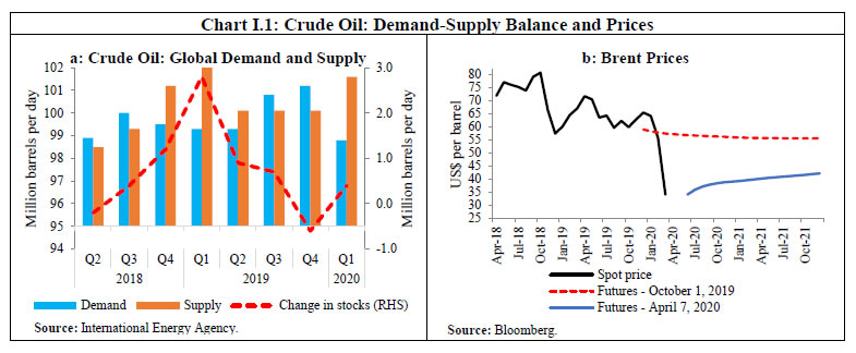 Second, the nominal exchange rate (the Indian rupee or INR vis-à-vis the US dollar) exhibited sizable two-way movements during October-December 2019. The INR came under intensified and sustained depreciation pressures beginning mid-January, reflecting a generalised weakening of emerging market currencies amidst flights to safety. Accordingly, the baseline assumes an average of INR 75 per US dollar to reflect these recent developments. Third, even though uncertainties relating to US-China trade relations and Brexit have receded, the COVID-19 pandemic has taken over. This has cast a shadow on the macroeconomic outlook, with global supply chains, trade, tourism, and the hotel industry being severely affected. The World Trade Organisation’s (WTO) goods and services trade barometers indicate that world trade volume growth weakened in early 2020; it is expected to be debilitated further by the adverse impact of COVID-19. The IMF expects that the contraction in global output in 2020 could be as bad as or worse than in 2009. The depth of the recession and the pace of recovery in 2021 would depend on the speed of containment of the pandemic and the efficacy of monetary and fiscal policy actions by various countries. The slowdown could be more protracted in dire scenarios in which the duration of COVID-19 extends longer. The Organisation for Economic Cooperation and Development (OECD) estimates suggest that annual global gross domestic product (GDP) growth could be lower by up to 2 percentage points for each month in which strict containment measures continue. If the shutdown continues for three months with no offsetting factors, annual GDP growth could be between 4-6 percentage points lower than it otherwise might have been. I.1 The Outlook for Inflation Headline consumer price index (CPI) inflation breached the upper tolerance band of the target in December 2019 and peaked in January 2020, before ebbing prices of vegetables, fruits and petroleum products produced a downward shift of 100 bps in February. The trajectory of inflation in the near-term is likely to be conditioned by the pace of reversal of the spike in vegetables prices, the dispersion of inflationary pressures across other food prices, the incidence of one-off cost-push effects on various elements of core inflation and especially, the evolution of the COVID-19 outbreak. Looking ahead, three months and one year ahead median inflation expectations of urban households softened by 10 bps and 20 bps, respectively, in the March 2020 round of the survey conducted by the RBI1. The proportion of respondents expecting the general price level to increase by more than the current rate also decreased for both three months and one year ahead horizons vis-à-vis the January 2020 round (Chart I.2). Although largely adaptive, inflation expectations of households and firms can shape future inflation through price and wage setting behaviour. According to the Reserve Bank’s consumer confidence survey for March 2020, inflation expectations moderated over the previous round2. 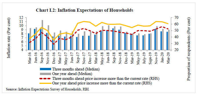 Manufacturing firms polled in the January-March 2020 round of the Reserve Bank’s industrial outlook survey expected an increase in selling prices as well as in the cost of raw materials in Q1:2020-21; nonetheless, pricing power of firms is expected to remain weak (Chart I.3)3. Purchasing managers’ surveys for manufacturing and services reported moderation in the rate of increase in input and output prices for March 2020. Professional forecasters surveyed by the Reserve Bank in March 2020 expected CPI inflation to ease from 6.6 per cent in February 2020 to 5.3 per cent in Q1:2020-21 and 3.2 per cent by Q4:2020-21 (Chart I.4)4. 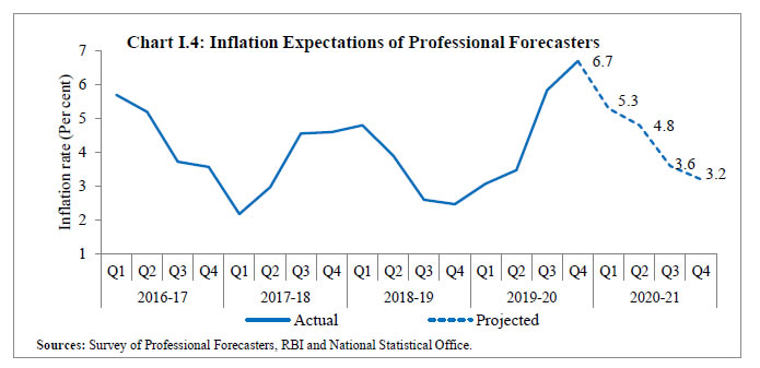 Thus, an array of forward-looking indicators is pointing to a much softer inflation trajectory. Looking ahead, the balance of inflation risks is slanted even further to the downside. First, food prices may soften under the beneficial effects of the record foodgrains and horticulture production, at least till the onset of the usual summer uptick. Second, the collapse in crude prices should work towards easing inflationary pressures, depending on the level of the pass-through to retail prices. All these signals are, however, heavily conditioned by the depth, spread and duration of COVID-19 and shifts in any of these characteristics of the pandemic can produce drastic changes in the outlook. In these conditions, forecasts are hazardous as they are subject to large revisions with every incoming data on the pandemic. The RBI Act, however, enjoins the Reserve Bank to publish and explain in the MPR, inter alia, the forecasts of inflation for 6-18 months from the date of its publication. Therefore, taking into account initial conditions, signals from forward-looking surveys and estimates from time series and structural models, CPI inflation is tentatively projected to ease from 4.8 per cent in Q1:2020-21 to 4.4 per cent in Q2, 2.7 per cent in Q3 and 2.4 per cent in Q4, with the caveat that in the prevailing high uncertainty, aggregate demand may weaken further than currently anticipated and ease core inflation further, while supply bottlenecks could exacerbate pressures more than expected. Per contra, a quick containment of COVID-19 could lead to faster recovery and, therefore, firmer inflation pressures. Given the lockdown, the compilation of the CPI for March and the following few months by the National Statistical Office could also become challenging. For 2021-22, assuming a normal monsoon and no major exogenous or policy shocks, structural model estimates indicate that inflation could move in a range of 3.6-3.8 per cent. I.2 The Outlook for Growth Prior to the outbreak of COVID-19, the outlook for growth for 2020-21 was looking up. First, the bumper rabi harvest and higher food prices during 2019-20 provided conducive conditions for the strengthening of rural demand. Second, the transmission of past reductions in the policy rate to bank lending rates has been improving, with favourable implications for both consumption and investment demand. Third, reductions in the goods and services tax (GST) rates, corporate tax rate cuts in September 2019 and measures to boost rural and infrastructure spending were directed at boosting domestic demand more generally. The COVID-19 pandemic has drastically altered this outlook. The global economy is expected to slump into recession in 2020, as post-COVID projections indicate. The sharp reduction in international crude oil prices, if sustained, could improve the country’s terms of trade, but the gain from this channel is not expected to offset the drag from the shutdown and loss of external demand. Turning to key messages from forward-looking surveys, the March 2020 round of the Reserve Bank’s survey showed that consumer confidence for the year ahead was expected to remain around its level recorded in the previous survey round in January 2020 (Chart I.5). However, an important caveat to the forward-looking surveys presented in this section is that they were completed before the nation-wide lockdown effective March 25. 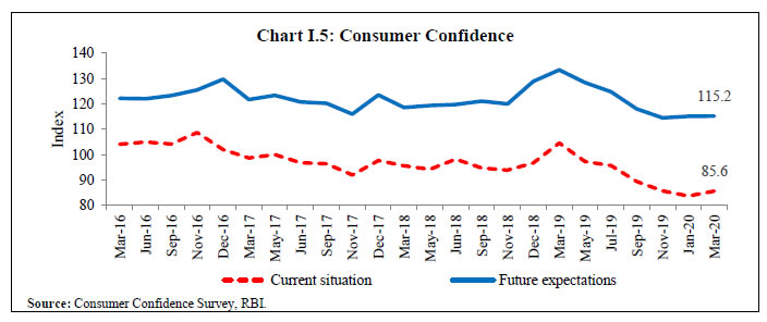 Optimism in the manufacturing sector for the quarter ahead had improved in the January-March 2020 round of the Reserve Bank’s industrial outlook survey, reflecting expectations of higher production, order books, capacity utilisation, employment conditions, exports and overall business situation (Chart I.6). In view of the intensification of COVID-19, a quick survey with select parameters was specially conducted during March 18-20 to capture business sentiments. From the limited responses received, a considerable worsening of the key demand indicators is seen in the outlook for Q1:2020-21. 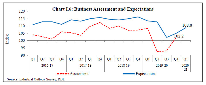 Surveys by other agencies (conducted prior to the intensification of COVID-19) indicated optimism on future business expectations (Table I.3). According to the purchasing managers’ surveys for March 2020, one year ahead business expectations of firms in manufacturing slumped to its weakest level, driven by fears of prolonged disruption from COVID-19. Business expectations of firms in the services sector also fell. | Table I.3: Business Expectations Surveys | | Item | NCAER Business Confidence Index
(February 2020) | FICCI Overall Business Confidence Index
(January 2020) | Dun and Bradstreet Composite Business Optimism Index
(March 2020) | CII Business Confidence Index
(March 2020) | | Current level of the index | 111.2 | 59.0 | 63.0 | 53.4 | | Index as per previous survey | 103.1 | 55.0 | 56.4 | 49.4 | | % change (q-o-q) sequential | 7.9 | 7.3 | 11.7 | 8.1 | | % change (y-o-y) | -12.4 | -2.2 | -14.6 | -18.1 | Notes:
1. NCAER: National Council of Applied Economic Research.
2. FICCI: Federation of Indian Chambers of Commerce & Industry.
3. CII: Confederation of Indian Industry. | Professional forecasters polled in the March 2020 round of the Reserve Bank’s survey (conducted during March 6-19 before the announcement of the nation-wide lockdown) expected real GDP growth to recover from 4.6 per cent in Q4:2019-20 to 6.1 per cent in Q4:2020-21 (Chart I.7 and Table I.4). 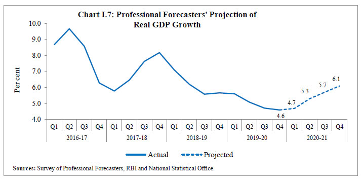
| Table I.4: Projections - Professional Forecasters | | (Per cent) | | Median Projections of Professional Forecasters | 2019-20 | 2020-21 | | Inflation, Q4 (y-o-y) | 6.7 | 3.2 | | Real GDP growth | 5.0 | 5.5 | | Gross domestic saving (per cent of GNDI) | 29.4 | 29.5 | | Gross capital formation (per cent of GDP) | 30.0 | 30.0 | | Credit growth of scheduled commercial banks | 7.2 | 9.3 | | Combined gross fiscal deficit (per cent of GDP) | 6.8 | 6.5 | | Central government gross fiscal deficit (per cent of GDP) | 3.8 | 3.6 | | Repo rate (end-period) | 5.15 | 4.65 | | Yield on 91-days treasury bills (end-period) | 4.9 | 4.7 | | Yield on 10-year central government securities (end-period) | 6.2 | 6.1 | | Overall balance of payments (US$ billion) | 49.8 | 40.0 | | Merchandise exports growth | -2.9 | -0.6 | | Merchandise imports growth | -7.2 | -2.9 | | Current account balance (per cent of GDP) | -1.0 | -0.7 | Note: GNDI: Gross National Disposable Income.
Source: Survey of Professional Forecasters (March 2020 round, conducted during March 6-19, 2020). | Overall, apart from the continuing resilience of agriculture and allied activities, other sectors of the economy will be adversely impacted by the pandemic, depending upon its intensity, spread and duration. Relatively modest upsides are expected to emanate from monetary, fiscal and other policy measures and the early containment of COVID-19, if that occurs. Such uncertainties make the forecasting of inflation and growth highly challenging (Box I.1). Box I.1: Forecasting Under Uncertainty in a Cyclical Downturn Monetary policy actions impact output and inflation with long and variable lags. Hence, timely and reliable forecasts of output and inflation are of critical importance. Domestic and global shocks to key conditioning variables such as global crude oil prices, global trade and growth, the exchange rate, the monsoon outturn and the rising frequency of their visitations make forecasting a challenging task, however, especially around the turning points. In an analysis of inflation and GDP growth forecasts of 17 select central banks for 2018 and 2019, most of them, including the RBI, were initially optimistic about economic activity (i.e., negative forecast errors)5. The standardised forecast errors (i.e., errors divided by the actual growth rate/inflation) were comparable (Chart I.1.1). 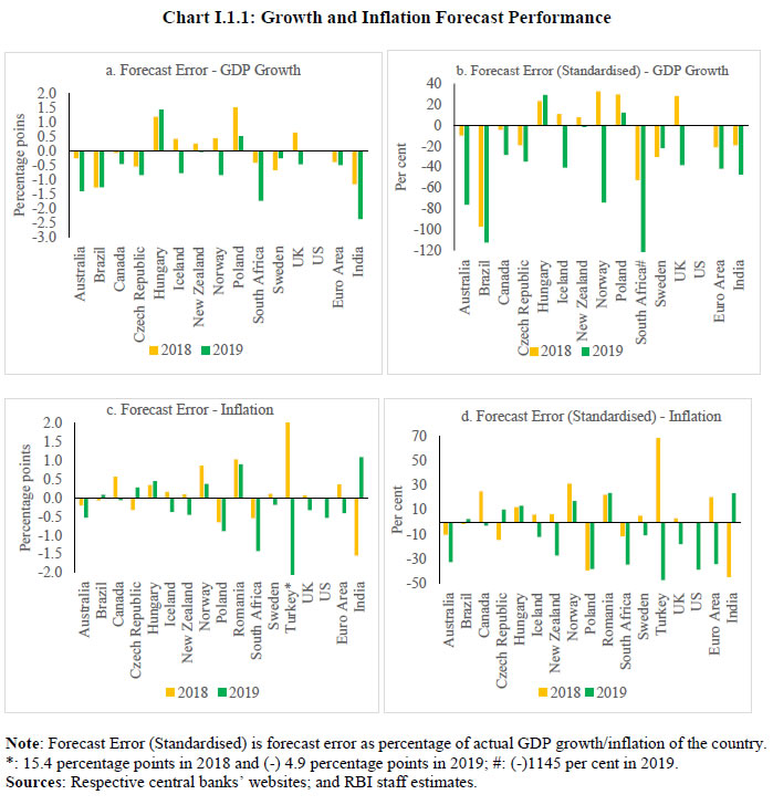 Panel regression results indicate that global growth surprises have been an important factor underlying domestic growth forecast errors; crude oil price surprises have a negative impact, although not significant (Equation 1). However, inflation forecast errors seem to be more due to country-specific idiosyncratic factors - domestic growth forecast errors as well as crude oil price surprises are not statistically significant (Equation 2). The constant term is statistically insignificant in both the regressions, suggesting that the forecast errors were unbiased, once the global growth and crude oil surprises were controlled for. Figures in parentheses are t-statistics; y_fe, π_fe, yw_s, doil are growth forecast errors, inflation forecast errors, global growth surprise and change in crude oil prices in local currency terms, respectively6. In India, the forecasting challenges are even more acute, given the high share (45.9 per cent) of the food basket in the CPI (Combined) (Chart I.1.2) as well as large revisions in past GDP growth rates. The Reserve Bank, like other central banks, provides fan charts around the baseline projections to convey future uncertainty. | Against this backdrop and especially, the highly fluid circumstances in which incoming data produce shifts in the outlook for growth on a daily basis, forecasts for real GDP growth in India are not provided here, awaiting a clear fix on the intensity, spread and duration of COVID-19. To illustrate, in early March, the OECD projected the decline in global growth for 2020 in the range of 0.5-1.5 percentage points. More recently, with COVID-19 having spread to more than 200 countries, the IMF’s latest assessment is that global growth during 2020 could be negative vis-à-vis growth of 2.9 per cent in 2019 (which itself was a decadal low). Thus, global growth could be lower by three percentage points or more in 2020 relative to 2019. The possible impact of the global slowdown on India’s growth and inflation can be assessed by using the Quarterly Projection Model (QPM)7 under alternative scenarios. Scenario 1 assumes global growth in 2020 to be 3 percentage points lower than in 2019. Scenario 2 assumes that the outbreak is contained faster and the loss of global output growth is only 1.5 percentage points relative to 2019. Lower global output and demand can impact the Indian economy through a variety of channels. First, it can affect exports adversely, leading to lower domestic demand, growth and inflation. Second, international crude oil and other commodity prices have already softened sharply amidst high volatility and India, being a net importer, can benefit from the lower commodity prices. Finally, heightened global financial market volatility can feed into domestic financial markets and impact both growth and inflation. The QPM captures all these channels. The model’s simulations suggest that, on account of global factors, domestic growth could be lower, at its peak, by 180 bps in Scenario 1 and by 80 bps in Scenario 2. Inflation could be lower by 40-100 bps at its peak under the two scenarios (Chart I.8). 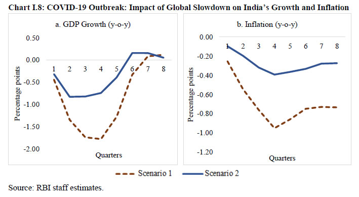 I.3 Balance of Risks The COVID-19 pandemic poses upside and downside risks to the baseline assumptions and outlook. (i) Exchange Rate The exchange rate of the Indian rupee vis-à-vis the US dollar has moved in both directions in recent months. Renewed bouts of global financial market volatility caused by the uncertainty of macroeconomic impact of the COVID-19, as in February-March 2020, could exert pressure on the Indian rupee. Should the INR depreciate by 5 per cent from the baseline, inflation could edge up by around 20 bps while GDP growth could be higher by around 15 bps through increased net exports. In contrast, should COVID-19 normalise quickly, strong capital flows could revive. An appreciation of the INR by 5 per cent could moderate inflation by around 20 bps and GDP growth by around 15 bps vis-à-vis the baseline. (ii) International Crude Oil Prices Global crude oil prices have declined sharply from their October 2019 levels mainly due to weakening of global demand following the outbreak of COVID-19, and Saudi Arabia’s decision to cut prices. However, the short and medium-term outlook of oil remains highly uncertain. A V-shaped global recovery due to an early containment of the COVID-19 or renewed geopolitical tensions or an agreement on production cuts could lead to a sharp reversal in international crude oil prices. Should the Indian basket of crude oil prices increase by 10 per cent above the baseline assumption, inflation could be higher by 20 bps and growth could be weaker by around 15 bps. If COVID-19 were to persist longer, global economic activity and demand for crude oil could fall further in an environment of sustained oversupply due to Saudi Arabia’s decision to enhance production. Should the Indian basket crude price fall by 10 per cent vis-à-vis the baseline, inflation could ease by up to 20 bps and growth higher by up to 15 bps, depending upon the extent of pass-through to domestic product prices. (iii) Food Prices After remaining subdued for a considerable period, food inflation in India increased sharply during October 2019-January 2020, driven by a spike in vegetable prices. The baseline path assumes vegetable prices to fall rapidly in response to arrivals of rabi harvests and a normal south-west monsoon during 2020, which is supported by early signals of likely ENSO (El Nino – Southern Oscillation) neutral conditions. Adequate buffer stocks in cereals and a good rabi harvest (2019 season) could soften food inflation more than anticipated and pull down headline inflation by 50 bps below the baseline. On the other hand, a deficient or spatially skewed south-west monsoon, and an unexpected hardening of prices of non-vegetable food items could push headline inflation above the baseline by around 50 bps in 2020-21. I.4 Conclusion COVID-19, the accompanying lockdowns and the expected contraction in global output in 2020 weigh heavily on the growth outlook. The actual outturn would depend upon the speed with which the outbreak is contained and economic activity returns to normalcy. Significant monetary and liquidity measures taken by the Reserve Bank and fiscal measures by the government would mitigate the adverse impact on domestic demand and help spur economic activity once normalcy is restored. Risks around the inflation projections appear balanced at this juncture and the tentative outlook is benign relative to recent history. But COVID-19 hangs over the future, like a spectre. _________________________________________________________
II. Prices and Costs Consumer price inflation surged between October 2019 and January 2020 propelled by a vegetable price spike, particularly of onions and breached the upper tolerance threshold in December before moderating in February. Fuel prices emerged out of deflation in December. After touching a historic low in October, inflation in CPI excluding food and fuel edged up due to cost-push factors. Costs of farm inputs, industrial raw materials, agricultural and non-agricultural labourers’ nominal wages and organised sector staff costs remained muted. Headline inflation, measured by the consumer price index (CPI),1 had been trailing below target for thirteen consecutive months till Q2:2019-20 when a ratcheting up of vegetables prices – mainly those of onions – dispelled this environment of price stability. In the event, headline inflation breached the upper tolerance ceiling of 6 per cent by December 2019 and peaked at 7.6 per cent in January 2020 before moderating to 6.6 per cent in February. An unusually prolonged south-west monsoon and unseasonal rains ravaged the later part of the kharif harvest and produced an unprecedented rise in prices of onions. In fact, excluding onions, headline inflation would have been 4.5 per cent in Q3 and 5.9 per cent in Q4 (till February), underscoring the severity of the onion price shock. Fuel prices too moved out of five months of deflation into positive territory in December 2019 and increased sharply thereafter. Inflation excluding food and fuel – or core inflation – hardened in a sustained manner from a historic low of 3.4 per cent in October 2019 to 4.3 per cent in January 2020, propelled by a series of cost pushes before registering some moderation in February (Chart II.1). 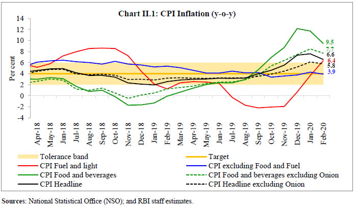 The Reserve Bank of India (RBI) Act, 1934 (amended in 2016) enjoins the RBI to set out deviations of actual inflation outcomes from projections, if any, and explain the underlying reasons thereof. The Monetary Policy Report (MPR) of October 2019 had projected CPI inflation to remain range-bound in H2: 2019-20, at 3.5 per cent in Q3:2019-20 and at 3.7 per cent for Q4:2019-20. Actual inflation outcomes have overshot projections by a considerable margin – 2.3 percentage points in Q3 and 3.4 percentage points in Q4 (Chart II.2). 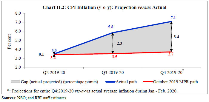 As stated earlier, the unanticipated and unparalleled spike in onion prices was the major source of deviation of headline inflation from projections. Unseasonal rains also delayed the seasonal winter moderation in prices of other vegetables, particularly those of potatoes. In addition, a larger than anticipated pick-up in cereals and milk prices due to kharif crop damage coming from the unseasonal rains, lower wheat imports and higher minimum support prices for wheat in the case of the former and an escalation in input costs in the case of the latter aggravated inflation pressures. CPI excluding food and fuel inflation also turned out to be a source of projection errors in Q4 due to a series of cost-push shocks – higher mobile phone tariffs; higher motor-vehicles prices due to the ongoing switchover to BS-VI2 compliant vehicles, higher gold prices reflecting international price movements; and higher services prices for sweepers, laundry, beauticians, bus fares – reflecting, inter alia, the spill over from higher food and fuel prices. In Q4:2019-20 (January-February), crude oil prices (Indian basket) softened from around US$ 63 per barrel at the time of the October MPR to US$ 55 per barrel by February, which helped temper these cost-push upsides. II.1 Consumer Prices A decomposition of year-on-year (y-o-y) inflation suggests that a sharp increase in price momentum as well as unfavourable base effects were at work in H2:2019-203. As against the normal seasonal decline in food prices during Q3, the measured food price momentum in Q3 was positive registering the highest increase during any third quarter in the history of the index. As a result, food inflation surged to double digits by the end of Q3. Adverse base effects also pushed up fuel inflation. In January, food prices started to decline, but the persisting firmness in the momentum of core inflation pushed headline inflation to a peak in January. In February, headline inflation moderated coming from a sharp decline in food prices and waning of core inflation momentum (Chart II.3). 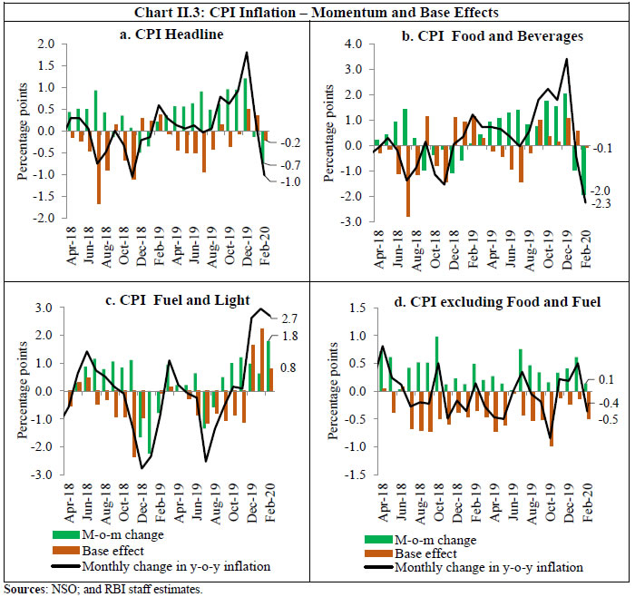 The distribution of inflation across CPI groups in 2019-20 has diverged considerably from the recent historical experience. Median inflation rate turned out to be lower compared with the last three-year average. However, 2019-20 exhibited high positive skew – as food sub-groups like vegetables exhibited very high inflation rates – compared to a negative skew for the historical average. As a result, the mean inflation rate for 2019-20 turned out to be considerably higher than the average of last 3 years (Chart II.4). Even as select food items swayed overall inflation rates in Q3:2019-20, a pick-up in the diffusion indices4 of price changes in CPI items, on a seasonally adjusted basis, also point to a broad-basing of price increases in the CPI basket – across goods and services – during this period. In Q4 so far, while almost all services have continued to register price increases, incidence of price increases in goods has seen some compression, largely on account of food items (Chart II.5). 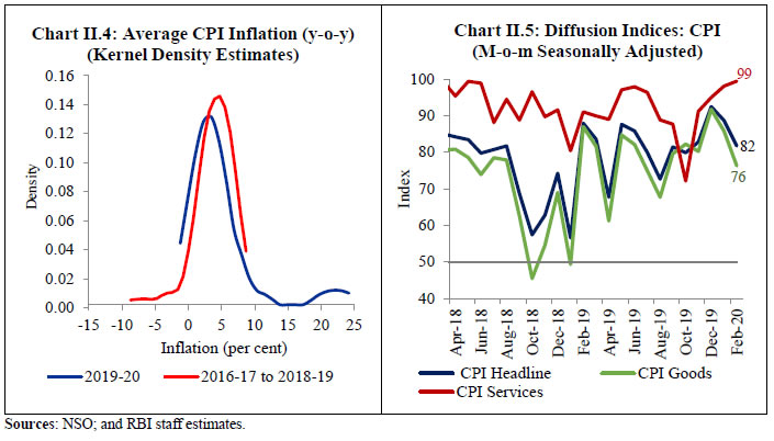 II.2 Drivers of Inflation A historical decomposition of inflation outcomes in H2:2019-20 reveals how adverse supply shocks overwhelmed the disinflationary impact of subdued domestic demand, both urban and rural (Chart II.6a).5 Perishable goods (non-durable goods with a 7-day recall6) – food items such as vegetables, milk and meat products – were the key drivers, contributing 1.3 percentage points to overall inflation in Q2, 3.7 percentage points in Q3 and 4.0 percentage points in Q4 so far (Chart II.6b). The contribution of less perishable goods (non-durable goods with a 30-day recall) also picked up from Q3:2019-20 due to cereals, pulses, sugar and petroleum products. Durable goods contribution to headline inflation, which remained largely steady during September-December – on an average at 36 bps – picked up to around 40 bps in January-February due to a rise in gold prices. Imported goods7 contributed negatively to overall inflation during September-November 2019, but their contribution turned positive during December 2019-February 2020 – on an average contributing around 60 bps to headline inflation, after a surge in energy and precious metals prices (Chart II.6c). The contribution of services to overall inflation remained sticky at around one percentage point as the sharp increase in mobile telecom charges during December 2019-January 2020 more than offset the moderation in inflation in house rentals, hospital services and tuition fees (Chart II.6b). 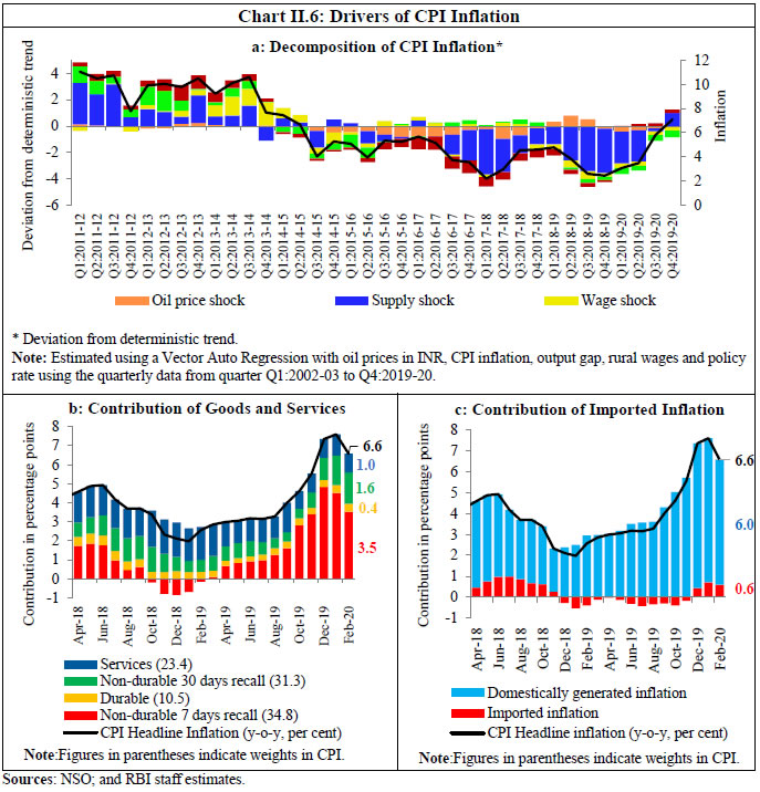 CPI Food Group Food and beverages (weight: 45.9 per cent in CPI) weighed heavily on changes in the overall CPI inflation during April 2019-February 2020, with the cumulative peak food price build-up in December turning out to be at a historical high (Chart II.7a & II.7b). As a result, food inflation, which had ranged between 0.7 per cent and 4.7 per cent during March-September 2019, accelerated thereafter to peak at 12.2 per cent in December (Chart II.8a). Most of this upsurge was propelled by a vegetables price spike as a consequence of unseasonal rains; however, broad-basing of price pressures across the food category was observed in H2:2019-20 encompassing pulses, meat and fish, spices, eggs, cereals and milk (Chart II.8b). Subsequently, food inflation moderated sequentially in January and February 2020, with the delayed seasonal easing in vegetables prices. Price increases in respect of cereals (weight of 9.7 per cent in the CPI and 21.1 per cent in the food and beverages group) were sharper in H2: 2019-20. Wheat prices were driven up by higher procurement at upwardly revised minimum support prices (MSPs) and significantly lower imports [(-)39 per cent lower during April 2019-January 2020]. Non-public distribution system (PDS) rice prices emerged out of 11 months of deflation in October 2019 and gained momentum thereafter in the wake of damage to kharif crops due to unseasonal rain in October and early November 2019. They started to moderate from February 2020 due to large carry forward stocks, better rabi harvest prospects and lower exports. 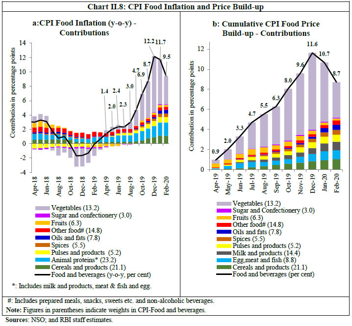 Inflation in prices of vegetables (weight of 6.0 per cent in the CPI and 13.2 per cent in the food and beverages group) rose to double digits from September 2019 and peaked at 60.5 per cent in December 2019, reflecting the impact of crop losses and supply disruptions due to excessive and unseasonal rains (Chart II.9a). With the arrival of the late kharif harvest, a delayed seasonal easing in vegetables prices started in January 2020. The year 2019-20 will likely be unique in vegetable price pressures, as the severe supply shock completely overshadowed the seasonal pattern of usual winter easing in prices of vegetables, particularly onions, tomatoes and potatoes which brings relief from the price build-up during the preceding months of the year (Chart II.9b). 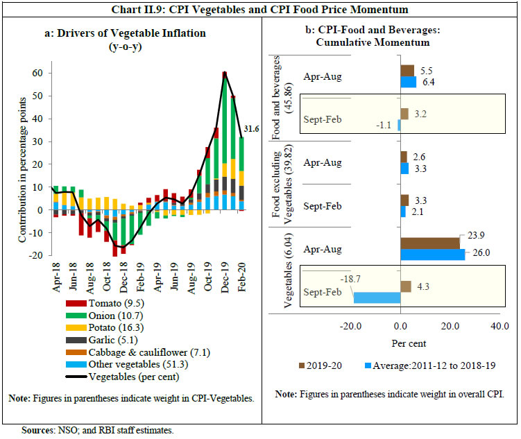 In India, a societal intolerance to inflation in double digits stands out starkly including in political discourse. This is best exemplified in social responses to inflation in onion prices. In 2019-20, onion prices surged from September 2019, with inflation in this category spiking to 327 per cent in December 2019 and contributing a staggering 4.7 percentage points to food inflation and 2.1 percentage points to headline inflation. This unpleasant inflation surprise exposed the time lags and lack of adequate band-width of supply-side measures such as imposing minimum export price (MEP) of US$ 850 per tonnes, banning export of onions, and imposing stock holding limits on wholesale traders and retailers in September 2019, as well as announcing import of 1.2 lakh tonnes of onions from Turkey, Afghanistan and Egypt during November-December 2019. It was only with the arrival of late kharif crop from January 2020 that onion prices began moderating. The ferocious pace of onion price escalation and the extent of spillovers highlight the urgent need for supply side reforms (Box II.1). Box II.1: Onion Price Shock – Issues in Supply Management The onion price shock of 2019 is the largest in recent times in terms of magnitude and duration (Chart II.1.1) In order to understand this, in many ways, unprecedented experience, the dynamics of the transmission of onion price shocks from various wholesale markets to all India average retail prices are evaluated with a vector autoregressive (VAR) model using daily data on price of onions from wholesale and retail markets with the following specification: where Yt represents the vector of daily prices of onion in the key wholesale markets, viz. Jodhpur, Kurnool, Nashik, Pune and Others (average of other markets), and the average all-India retail prices; et represents the vector of supply and demand shocks – shocks corresponding to wholesale market prices represent the supply shocks and the shock corresponding to average retail market price represents the demand shock. The estimates are based on daily wholesale and retail price data provided by Department of Consumer Affairs (DCA), Government of India from August 5, 2019 to February 28, 2020. The historical decomposition of average retail prices points to onion price shocks from the wholesale markets of Maharashtra in early-October and thereafter spreading to Karnataka by early-November and almost immediately getting transmitted to all-India retail prices, exacerbated by widening of price margins between wholesale and retail markets. By end-January, the onion price shocks completely reversed (Chart II.1.2). 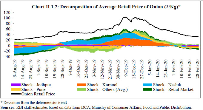 Given that onion production in India in any given year comfortably meets demand with additional produce available for exports, this analysis underscores the need for refining the supply management policies in managing the volatility in onion prices. The contours of more effective supply management for onions need to centre around the following: (1) making available better information systems to farmers on weather and the production outlook so as to enable them better plan onion production for the year ahead; (2) initiating reforms in the agricultural marketing systems to encourage direct sale of farm produce by farmers to consumers; (3) strengthening initiatives like e-NAM for better price discovery; (4) improving storage facilities for farmers so as to avoid distress sales; (5) creating an adequate buffer stock of rabi produce to help manage supply disruptions during leaner kharif and late-kharif seasons; and (6); encouraging food processing initiatives – dehydrating onions to convert into powder and paste forms that can be made available at a reasonable price. In fact, most of the onion price spikes in the past have occurred in kharif and late-kharif seasons, pointing to the key role of supply-side management policies in mitigating onion price spikes. | As regards other inflation-sensitive vegetables, potato prices remained in deflation from April 2019 to October 2019 despite a pick-up in prices during this period largely due to favourable base effects. The momentum of potato prices remained broadly positive during April 2019-January 2020, firmed up by crop loss and supply disruptions from excess/unseasonal rains during October-November 2019 in Punjab, Uttar Pradesh and West Bengal, which was reflected in lower mandi arrivals. Anecdotal evidence also suggests that cyclone bulbul resulted in delayed sowing in West Bengal by around 20 days. As a result, potato price inflation rose to 62.9 per cent in January 2020, before moderating to 47.0 per cent in February 2020 due to fresh arrivals on the back of production turning out to be higher by 3.5 per cent in 2019-20. On the other hand, inflation in tomato prices moderated from its peak of 70 per cent in May 2019 and remained in high double digits during October-December 2019, reflecting untimely rains and associated supply disruptions. Beginning January 2020, tomato price inflation started moderating in the usual seasonal downturn and turned into deflation in February 2020 at (-)4.3 per cent. Prices of fruits (weight of 2.9 per cent in the CPI and 6.3 per cent within the food and beverages group) emerged out of 9 months of deflation in September 2019 to reach a level of 5.8 per cent in January 2020, primarily due to unfavourable base effects. By February 2020, fruit price inflation eased to 4.0 per cent. Banana prices have seen a sustained decline since November 2019. On the other hand, apple prices started a decline from August 2019 itself on the back of higher market arrivals consequent on production being higher by 18.0 per cent during 2019-20, although prices recovered somewhat since January 2020. Prices of pulses (weight of 2.4 per cent in the CPI and 5.2 per cent in the food and beverages group) were another source of inflation pressures with inflation in this category picking up considerably to reach 16.6 per cent in February 2020 from (-) 0.8 per cent in April 2019. This reflected a decline in kharif pulses production – by 2.1 per cent as per second advance estimates (AE) for 2019-20 over final estimates for 2018-19 – and especially urad production (by 27.1 per cent) on account of lower kharif sowing and unseasonal rains-led crop damages (Chart II.10). Even though imports were higher by 25 per cent during April 2019-January 2020 y-o-y, they failed to mitigate the rising price pressures in pulses. 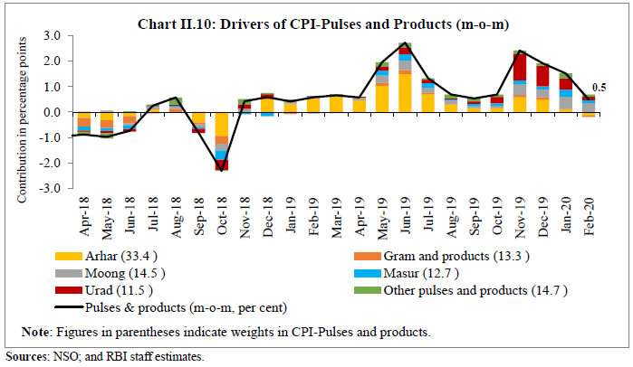 Besides vegetables and pulses, prices of animal-based protein-rich items were another pressure point, contributing 20.4 per cent to overall food inflation in 2019-20. Inflation in the case of meat and fish remained elevated during April 2019-January 2020 and reached 10.6 per cent in January 2020 (highest in last 72 months). The prices of meat and fish increased significantly during the year (except during the lean season of August-October 2019) reflecting higher feed prices (especially, maize and soybean) on account of unseasonal rains, which accentuated seasonal price pressures. Concomitantly, egg price inflation also inched up to 10.5 per cent in January 2020 from 1.9 per cent in April 2019, but softened to 7.3 per cent in February 2020. Prices of both chicken and egg contracted sharply in February 2020 on account of a fall in consumption due to COVID-19 scare. Prices of milk and milk products (weight of 6.6 per cent in the CPI and 14.4 per cent in the food and beverages group) also contributed to higher food inflation. Co-operatives like Amul and Mother Dairy raised retail milk prices for the second time (first round in May 2019) in December 2019 in the range of ₹ 2-3 per litre due to increased procurement prices. Many state milk co-operatives also announced increases in prices, which kept the momentum of milk and its products at an elevated level during the year. Procurement prices were raised in response to the increase in the cost of production. Additionally, higher global prices for skimmed milk products also impacted domestic milk prices positively. Milk inflation hardened to a 56-month high of 6.0 per cent in February 2020. Sugar and confectionery prices (weight of 1.4 per cent in the CPI and 3.0 per cent in the food and beverages group) emerged out of four months of continuous deflation in October 2019, partly due to adverse base effects. Despite domestic and global production shortfalls, higher than expected domestic availability due to last year’s carry forward stock has helped keep domestic price pressures under check. Inflation in prices of edible oils and fats also edged up during the year from 0.7 per cent in April 2019 to 7.6 per cent in February 2020. Higher edible oils inflation emerged from a combination of rising international prices, lower domestic production of rabi oilseeds and adverse base effects. Higher milk prices also impacted the prices of ghee and butter. Price pressures picked up considerably in spices leading to a gradual hardening of inflation in this group to 8.8 per cent in February 2020 from 0.8 per cent in April 2019 due to overall lower production. CPI Fuel Group Prices of the CPI fuel group, which sank into deflation in July at (-)0.3 per cent, continued in negative territory till November 2019 as prices of key fuel items such as liquefied petroleum gas (LPG), firewood and chips and dung cake moved into deep deflation. The fuel group moved out of deflation in December registering a sharp rise thereafter, taking inflation in this category to 6.4 per cent by February. A pick-up in prices of electricity, LPG and firewood and chips and strong adverse base effects contributed to this upsurge (Chart II.11a). International propane and butane prices, which were declining through H1:2019-20, registered sustained price increases during October 2019-January 2020, accentuated by supply disruptions due to geopolitical tensions. These pressures were also transmitted to domestic LPG prices with a lag in February 2020 (Chart II.11b). Administered kerosene price inflation remained sticky and elevated reflecting calibrated price increases by oil marketing companies (OMCs) to phase out the fuel subsidy. By early February, however, administered prices were above market rates, particularly due to the sudden plunge in international prices. This led to some reduction in kerosene prices in the PDS in March (Chart II.11c). 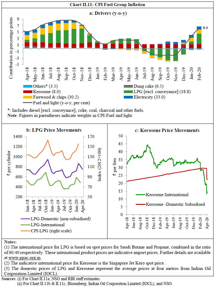 CPI excluding Food and Fuel CPI inflation excluding food and fuel or core inflation picked up sequentially from 3.4 per cent in October 2019 to 4.3 per cent in January 2020, before registering some moderation in February 2020 (Chart II.12). In terms of components, the price build-up during 2019-20 was much lower than historical averages, barring for the transport and communication, and personal care and effects sub-groups (Chart II.13). 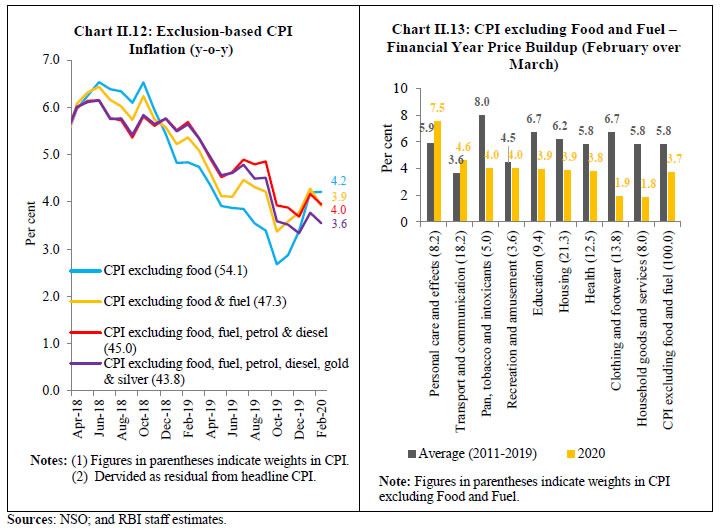 Volatile movements in international crude oil prices and the consequent increase in domestic pump prices mainly contributed to the upturn in CPI excluding food and fuel till January 2020 and the subsequent moderation in February. CPI petrol and diesel, which was in deflation for 11 months till November 2019, saw a sharp uptick in inflation during December 2019-January 2020 before moderating in February. Volatility in crude oil prices in H2:2019-20 emanated from a series of events starting with rising geo-political tensions in early September, followed by production cuts by the Organization of the Petroleum Exporting Countries (OPEC) in early December and renewed geo-political tensions in early January. Crude oil prices moderated sharply from mid-January on easing of geo-political tensions, price war between OPEC and Russia, and fears of a global recession due to COVID-19. While the pass-through of collapse in international crude oil prices to domestic pump prices is still unfolding, its extent has been tempered by increases in taxes on petrol and diesel (Chart II.14a). Excise duties for petrol and diesel were increased by ₹ 3 per litre each on March 14, 2020 as international crude oil prices tumbled below US$ 40 per barrel. With this increase, the total excise duty on petrol and diesel works out to ₹ 22.98 per litre and ₹ 18.83 per litre, respectively. The divergence between international and domestic pump prices has now widened to highest levels seen in the recent period (Chart II.14b). CPI inflation excluding food, fuel, petrol and diesel troughed in December, before registering a sharp increase in Q4 so far (January-February). CPI inflation excluding food, fuel, petrol, diesel, gold, silver – which further excludes the volatile gold and silver price effects – also saw similar movements (Chart II.12). A break-up of CPI excluding food, fuel, petrol and diesel into its good and services components, shows the impact of cost-push factors which reversed a sharp moderation in inflation in this category and hardened it during December 2019- January 2020 (Chart II.15). Core goods prices inflation moderated sequentially till December 2019, caused by a broad-based fall in inflation across goods items, particularly health inflation due to large and favourable base effects. Goods inflation has been ticking up since January due to firming up of prices of clothing, pan, tobacco, medicines in the health sub-group following an increase in administered prices of essential medicines and automobiles in the transport and communication sub-group due to a rise in input costs and a switch-over in emission norms to BS-VI (Chart II.15a). Core services inflation moderated sharply during October-November 2019 due to a fall in inflation in domestic maid/cook and other household services; tuition fees in education services; house rentals; transport fares and mobile telephone charges under transportation and communication services. Mobile telephone charges have, however, increased (by close to 12 per cent between November 2019 and February 2020), following the increase in tariffs by major private mobile operators in early December. Bus fares and administered railway fares also increased during this period. As a result, transport and communication services inflation registered significant increases, pushing up overall services inflation. Reflecting subdued demand conditions, housing inflation softened throughout H2:2019-20. Education services inflation also remained soft during December 2019-February 2020 (Chart II.15b). Other Measures of Inflation Inflation in sectoral CPIs, i.e., for industrial workers (CPI-IW), agricultural labourers (CPI-AL) and rural labourers (CPI-RL), increased sharply during August-December 2019, driven up primarily by the unseasonal rise in food prices. The pace of increase, however, softened in January-February 2020, on the back of cooling of prices in the food group. Inflation in food and fuel components of CPI-AL and CPI-RL was higher than that in headline CPI. A larger share of food nudged overall inflation measured by these indices to double digit levels during December 2019-February 2020. In the case of CPI-IW, with the complete waning of the house rent allowance impact of the seventh central pay commission (CPC) after December 2019, inflation registered a sharp fall, closing the gap with headline CPI. Notwithstanding this ebbing, the latest increase in momentum in housing index in CPI-IW – which is revised once in six months, in January and July every year – contributed the largest upward push to CPI-IW in January 2020 (with a m-o-m increase of 3.7 percentage points). CPI-IW inflation decreased further in February 2020 due to sharp correction in food prices by 1.7 percentage points. Inflation in terms of the wholesale price index (WPI) fell during August-October 2019 in sharp contrast to the sectoral CPIs, due to a decline in prices of non-food manufactured products on account of the softening of global commodity prices. Subsequently, WPI inflation edged up in line with sectoral CPIs as wholesale food prices rose in December 2019-January 2020 before moderating again in February with easing of food prices. Gross Domestic Product (GDP) and Gross Value Added (GVA) deflators picked up in Q3:2019-20 after reaching a record low in Q2:2019-20, indicating a clear divergence with CPI and a broad alignment with WPI (Chart II.16a). Trimmed mean measures of inflation, obtained by statistically removing outliers and eliminating positive and negative skew, provide a measure of underlying inflation movements. Exclusion based measures of CPI also capture persistent trends in inflation by removing components that are considered idiosyncratic. Over the last six months, both trimmed means and exclusion-based measures, have firmed up (Charts II.12 and II.16b). II.3 Costs Underlying cost conditions have largely been in sync with inflation in terms of the WPI (Chart II.17). Inflation in terms of farm inputs and industrial raw material prices (extracted from WPI) moderated significantly after April 2019 and remained in negative territory during September-November 2019, before registering a pick up during December 2019-February 2020. The pick-up during December 2019-January 2020 partly reflected recovery in prices of global crude oil and petrochemicals as well as adverse base effects. In addition, cost of minerals and non-food articles also influenced the recent price dynamics of non-farm input costs. Among other industrial raw materials, domestic coal inflation picked up to 2.4 per cent during October 2019-February 2020 from 0.4 per cent in April 2019 in line with the increase in international coal prices. Prices of paper and paper products remained in deflation during July 2019-February 2020 due to lower raw material cost, including that of pulp. In the case of fibres, deflation persisted during August 2019-February 2020, following easing in prices of raw cotton and coir fibre, which also reflected in the contraction in cotton yarn prices during the same period. As regards farm sector inputs, inflation hardened in the case of fodder due to unseasonal rains, while some easing was observed in the case of fertilisers and pesticides reflecting generally subdued momentum in international fertiliser prices. Prices of electricity, which carry a high weight in both industrial and farm inputs, recorded a modest increase during the year, reflecting weak demand conditions. Inflation in terms of agricultural machinery and implements costs has also softened gradually during the current financial year. 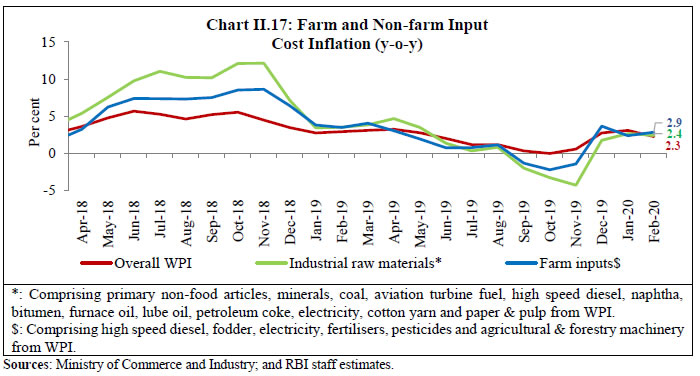 Growth in nominal rural wages, both for agricultural and non-agricultural labourers, remained subdued averaging around 3.4 per cent and 3.3 per cent, respectively, during 2019-20 so far (up to January 2020) mainly reflecting continued slowdown in the construction sector (Chart II.18). With a sharp rise in rural retail inflation, however, real rural wage growth has been negative as derived from CPI-AL and CPI-RL measures since March 2019 and CPI-rural inflation since September 2019. 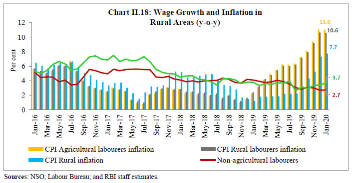 Growth in organised sector staff costs showed divergent movements for services and manufacturing firms. While staff cost growth of services firms increased in Q3:2019-20 over the previous quarter, it declined for manufacturing firms. Unit labour costs (ratio of staff cost to value of production in percentage terms) for companies in the manufacturing sector increased sequentially from 5.9 per cent in Q4:2018-19 to 6.3 per cent in Q1:2019-20 and further to 6.8 per cent in Q2 due to sequential decline in the value of production, alongside an increase in staff cost. In Q3:2019-20, unit labour cost for manufacturing moderated marginally. On the other hand, higher quarterly growth in value of production for firms in the services sector led to a fall of 220 basis points in unit labour cost from 30.1 per cent in Q2:2019-20 to 27.9 per cent in Q3 even as staff cost increased somewhat (Chart II.19). 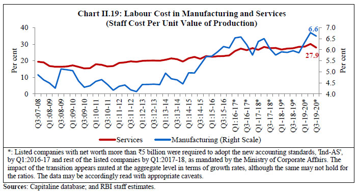 Manufacturing firms participating in the Reserve Bank’s industrial outlook survey reported muted cost pressures in Q3:2019-20 and Q4. This reflected softening of inflation in farm and industrial raw materials in Q3 and weak metal and other commodity price pressures in Q4. A decline in cost of finance was also reported by the companies polled in Q3 and Q4. Cost pressures on account of salary outgoes also fell in Q3 and are expected to have remained weak in Q4. Weak demand conditions and muted input price pressures kept selling prices soft, with expectations showing only a muted uptick in Q4. While producers’ price expectations were subdued, inflation expectations of households, as measured in the Reserve Bank survey, softened. Manufacturing firms polled for the purchasing managers’ index (PMI) reported modest increases in input prices and stable output prices in Q4. Input prices, however, firmed up markedly in case of the PMI services firms in Q4 (up to February) driven by higher food, labour and material costs before slowing sharply in March 2020 amid lower food and fuel prices, and reduced demand. Prices charged by services firms remained broadly range bound in Q3 and Q4 but softened in March 2020 with some firms reducing their fees due to weak demand conditions. II.4 Conclusion The inflation landscape changed dramatically during H2:2019-20 primarily on account of wide swings in onion prices. In Q4:2019-20, before the intensification of COVID-19, forward looking surveys were already indicating weak consumer confidence and low pricing power of firms. Since March 2020 the inflation outlook has become highly uncertain due to the COVID-19 outbreak turning into a pandemic. Crude oil prices have collapsed to lows not seen since early 2000s. With several major economies in lockdown mode, demand conditions may weaken sharply. Accordingly, countries across the world are bracing up for deflationary forces to take hold. India may not be immune to these extreme downside pressures imparted by the pandemic. With the entire country in lockdown, the NSO would face considerable challenges in compilation and measurement of consumer prices. ________________________________________________________________
III. Demand and Output The deterioration in aggregate demand conditions in 2019-20, was exacerbated by contraction in investment, and moderation in government expenditure in H2. On the supply side, agriculture and allied activities accelerated, buoyed by the late surge in south-west monsoon rainfall and bountiful north-east monsoon precipitation. However, industrial growth decelerated, led by a slowdown in manufacturing activity. Services sector activity moderated, pulled down by a slowdown in construction; trade, hotels, transport and communication; and public administration, defence and other services. The February 2020 data release by the National Statistical Office (NSO) reveals that a sequential slowdown set in upon the Indian economy from Q1:2018-19. Over H2:2018-19 and H1:2019-20, real GDP growth lost momentum further, averaging 5.5 per cent. The sub-5 per cent reading for Q3:2019-20 (4.7 per cent) has caused heightened uncertainty about the outlook. The oppressive force of the novel coronavirus (COVID-19) on weak or moderating high frequency indicators of activity, barring agriculture, indicates that the implicit real GDP growth for Q4:2019-20 in the NSO’s data release could be undershot by a fair margin. In fact, the widening incidence of COVID-19 in March 2020 may produce downward pulls to Q4 GDP. Underlying this marked downturn relative to recent experience is the contraction in gross fixed capital formation (GFCF) from Q2:2019-20. Consumption demand accelerated and sustained overall demand, driven mainly by a sharp pick up in government final consumption expenditure (GFCE). Net exports also contributed positively to aggregate demand, but essentially because the contraction in imports outpaced the decline in exports. On the supply side, agriculture and allied activities imparted momentum to gross value added (GVA) in Q2 and Q3, buoyed by increases in kharif and horticulture production. The industrial sector remained moribund, bound down by weak demand conditions, and hence weak pricing power. In the services sector, activity has been weakening through H2:2019-20 with high frequency indicators for January and February 2020 either moderating or declining, barring PMI, cement production and railway freight traffic. Public administration, defence and other services (PADO) remained robust in Q2 and Q3. However, during January-February 2020, centre’s revenue expenditure excluding interest payments and subsidies grew marginally. Beginning March, the lockdown in the wake of the outbreak of COVID-19 has choked manufacturing activities. Anecdotal evidence suggests that in the manufacturing sector, dislocations of labour adversely impacted automobiles, electronic goods and appliances, and apparel. Services such as trade, tourism, airlines, the hospitality sector and construction have been hit hard. III.1 Aggregate Demand The deterioration in aggregate demand conditions in 2019-20, was exacerbated by contraction (1.3 per cent) in gross fixed capital formation, and moderation in government expenditure in H2. Although private consumption held up in sequential terms, it was slower in H2:2019-20 on a y-o-y basis (Chart III.1a and Table III.1). Overall, the drag on GDP growth in H2:2019-20 can be decoded to unfavourable base effects, since momentum – measured by the q-o-q seasonally adjusted annualised growth rate (SAAR) - accelerated in H2 (Chart III.1b). With COVID-19 having taken a grievous toll in February and particularly in March, it is unlikely that this momentum was sustained as the year closed. Accordingly, the NSO’s estimate of real GDP growth for the year as a whole at 5.0 per cent in 2019-20, which itself was down from 6.1 per cent in 2018-19, may be at risk. 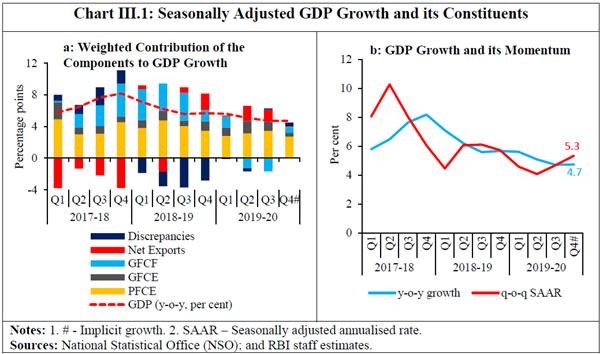 In the absence of hard data on underlying activity from traditional sources, availability of high frequency information in large volumes, either structured or unstructured, varying in form and content, has opened up avenues for extracting meaningful signals on the state of the economy. A sentiment index (SI), prepared on the basis of daily news feed in print media is able to track economic activity relatively well in the Indian context. The SI indicates weak activity in Q4:2019-20 (Box III.1). | Table III.1: Real GDP Growth | | (y-o-y, per cent) | | Item | 2018-19
(FRE) | 2019-20
(SAE) | Weighted Contribution* | 2018-19 (FRE) | 2019-20 (SAE) | | 2018-19 | 2019-20 | Q1 | Q2 | Q3 | Q4 | Q1 | Q2 | Q3 | Q4# | | Private final consumption expenditure | 7.2 | 5.3 | 4.0 | 3.0 | 6.7 | 8.8 | 7.0 | 6.2 | 5.0 | 5.6 | 5.9 | 4.9 | | Government final consumption expenditure | 10.1 | 9.8 | 1.0 | 1.0 | 8.5 | 10.8 | 7.0 | 14.4 | 8.8 | 13.2 | 11.8 | 4.9 | | Gross fixed capital formation | 9.8 | -0.6 | 3.0 | -0.2 | 12.9 | 11.5 | 11.4 | 4.4 | 4.3 | -4.1 | -5.2 | 2.5 | | Exports | 12.3 | -1.9 | 2.4 | -0.4 | 9.5 | 12.5 | 15.8 | 11.6 | 3.2 | -2.1 | -5.5 | -2.8 | | Imports | 8.6 | -5.5 | 2.0 | -1.3 | 5.9 | 18.7 | 10.0 | 0.8 | 2.1 | -9.3 | -11.2 | -3.0 | | GDP at market prices | 6.1 | 5.0 | 6.1 | 5.0 | 7.1 | 6.2 | 5.6 | 5.7 | 5.6 | 5.1 | 4.7 | 4.7 | FRE: First Revised Estimates; SAE: Second Advance Estimates; #: Implicit growth.
*: Component-wise contributions to growth do not add up to GDP growth in the table because change in stocks, valuables and discrepancies are not included.
Source: NSO. |
Box: III.1: Media Sentiments on Economic Growth
– A Machine Learning Approach Big data tools and machine learning (ML) techniques such as natural language processing (NLP) and text mining have facilitated extraction and construction of numerical indicators out of news text (Shapiro et. al. 2018). The broad approach is to extract sentiment from daily news items pertaining to variables of interest (Godbole et. al. 2007). Each news item is classified into one of three sentiment classes, viz., positive, negative and neutral, based on the words present in the news. News items with no sentiments or those that are unrelated are discarded. A sentiment class explicitly represents words with similar semantic orientation as illustrated below (Chart III.1.1). Relevant news items under positive/ negative/ neutral sentiment class are consolidated and summarised into a Sentiment Index (SI)1, as defined below: SI = news items with “positive” sentiment (%) – news items with “negative” sentiment (%) For this analysis, daily news feeds for the period April 2015 to March 2020 have been sourced from media intelligence firm (Meltwater) and aggregated to derive a quarterly Sentiment Index to track upturns and downturns in year-on-year (y-o-y) growth in real GDP and GVA (Chart III.1.2). The association between sentiment index and economic activity (GDP or GVA growth) is measured in terms of correlation. Directional precision is measured in terms of a Sign Success Ratio (SSR)2 which is the proportion of time periods when the direction indicated by SI matches the directional change in GDP/GVA growth and is defined as follows:
The Sentiment index is found to be strongly correlated with both GDP and GVA growth and it is able to gauge the directional change satisfactorily (Table III.1.1). Sentiment index reveals subdued economic activities for the fourth quarter of 2019-20. | Table III.1.1: Statistical Association between SI and GDP/GVA Growth | | | GDP growth (Y-o-Y) | GVA growth (Y-o-Y) | | Correlation with SI | 0.62* | 0.71* | | SSR of SI (%) | 58 | 74 | *Statistically significant at 5 per cent level of significance
Sources: NSO; and RBI staff estimates. | Unconventional big data sources, such as news in online print media that are available on a high frequency basis complement survey-based gauges of the pulse of the economy. However, machine learning techniques are usually difficult to comprehend with macroeconomic interlinkages and are generally treated as additional monitoring techniques. References: Buono, D., Kapetanios, G., Marcellino, M., Mazzi, G., and Papailias, F. (2018), “Big Data Econometrics: Now Casting and Early Estimates”, Milan, Bocconi University, Baffi-Carefin Centre working paper 82. Godbole, N., Srinvasaiah, M., and Skiena, S. (2007), “Large-Scale Sentiment Analysis for News and Blogs”, Conference Proceedings of the International Conference on Weblogs and Social Media, January. Kumari, Shweta and Giddi, Geetha (2020), “Inflation Decoded through Power of Words”, Mimeo. Shapiro, Adam Hale, Moritz Sudhof, Daniel Wilson (2018), “Measuring News Sentiment”, Federal Reserve Bank of San Francisco Working Paper 2017-01. | GDP Projections versus Actual Outcomes The October 2019 Monetary Policy Report (MPR) projected GDP growth at 5.3 per cent for Q2:2019-20, 6.6 per cent for Q3 and 7.2 per cent for Q4, with risks evenly balanced around this baseline path (Chart III.2). Actual outcomes in terms of the NSO’s second advance estimates (SAE) undershot these projections by 20 and 190 basis points in Q2 and Q3, respectively. The downward surprise in Q2 stemmed from a stronger than anticipated drag from gross fixed capital formation and marginal weakness in private final consumption expenditure. In Q3, projection errors emanated mainly from a steep unanticipated contraction in gross fixed capital formation, which was the deepest in the new series of GDP. III.1.1 Private Final Consumption Expenditure Private final consumption expenditure (PFCE) remains the mainstay of aggregate demand, with its share at 57.6 per cent in H2:2019-20. The slowdown in PFCE in H2:2019-20 was caused by a combination of factors — weak rural demand due to depressed food prices/inflation in the previous two years; deceleration in rural wages; and downturn in labour-intensive exports which impacted rural consumption; and slowdown in urban consumption due to decelerating incomes (Chart III.3). 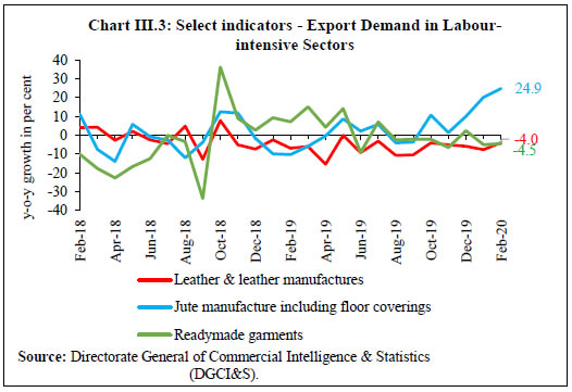 High frequency indicators of urban consumption demand present a subdued picture for Q4:2019-20 (Chart III.4a). Sales of passenger vehicles continued to contract in February 2020. Domestic air passenger traffic growth slowed in January 2020. Consumer durables growth contracted in January 2020. Even though there has been some uptick in vehicle loan growth for households and growth in credit card outstanding in February 2020, overall, urban consumption appears to have lost steam in Q4 with the outbreak of COVID-19 having accentuated the moderation (Chart III.4b). 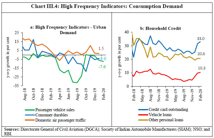 Among the indicators of rural consumption, motorcycle sales remained in contraction in February 2020 (Chart III.5). This sector faces some uncertainty following the change in emission norms, which was to be effective from April. Tractor sales, however, improved in January and steadied further in February 2020, reflecting improved rabi sowing. The consumer non-durable segment remained in contraction, reflecting weak rural demand (Box III.2). 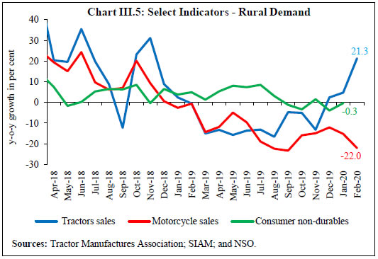 Box III.2: What Ails Rural Demand? The performance of agriculture is key to the state of rural demand. In recent years, the terms of trade (ToT) have moved against the farm economy, with back-to-back bumper harvests during 2016, 2017 and 2018 causing a decline in some food prices/inflation (Chart III.2.1). In the face of a global food supply glut, India’s exports of agricultural products were affected and consequently, they could not fulfil their usual vent for surplus role (Chart III.2.2). The excess supply resulting in an accumulation of stocks depressed agriculture commodities prices/inflation even further (Chart III.2.3). The index of inter-sectoral ToT, i.e., the ratio of agriculture GVA deflator to non-agriculture GVA deflator declined between 2016-17 and 2018-19 (Chart III.2.4). An alternative measure – the ratio of the wholesale price index (WPI) between agriculture and non-agriculture (excluding services) – corroborates this loss of ToT.
Alongside these developments, growth in rural wages has remained subdued, particularly for agricultural labour in both nominal and real terms, partly due to the slowdown in the construction sector (Chart III.2.5). Moreover, in recent years, the Mahatma Gandhi National Rural Employment Guarantee Act (MGNREGA) scheme does not seem to support rural income much due to delayed wage payments, lower wages and insufficient budgetary allocations. The Periodic Labour Force Survey (PLFS) report released by the NSO in May 2019 shows that wages under MGNREGA work are lower than the market wage rate for non-public work by 74 per cent for rural men and 21 per cent for rural women. The recent outbreak of COVID-19 and the subsequent lockdown enforced in the country are expected to bring down the aggregate demand drastically, both in rural and urban areas. The Government has announced a slew of measures like direct cash transfer to farmers, hiking wages under the MGNREGA scheme, and utilisation of welfare funds for construction workers to offset the adverse impact on rural demand. However, given the severity of the pandemic, rural demand is expected to go down further at least in the near future. In conclusion, unusually lower agriculture prices, slowdown in the construction sector and below average performance of the flagship MGNREGA programme have contributed to lower farm incomes, deceleration in rural wages and loss of employment opportunities in the rural sector and, more so, in the wake of COVID-19. | III.1.2 Gross Fixed Capital Formation Gross fixed capital formation (GFCF) growth turned negative in Q2 and Q3:2019-20. Consequently, the share of GFCF in GDP dropped to 30.2 per cent in 2019-20 from 31.9 per cent a year ago. Two key indicators of investment demand, viz., production and imports of capital goods have remained in contraction in January/February 2020 as well (Chart III.6a). As regards construction activity, finished steel consumption contracted in February, while cement production grew significantly. The performance of software firms – a proxy for investment in intellectual property products – has remained resilient, as evident from the latest financial results. Seasonally adjusted capacity utilisation (CU-SA) in the manufacturing sector declined below the long-term average in Q3:2019-20, corroborating that the need for fresh investment is depressed as also reflected in a slowdown in adjusted non-food bank credit (ANFC) (Chart III.6b). 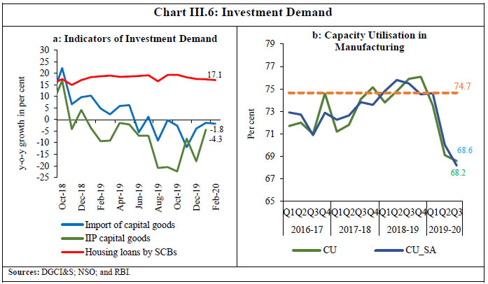 Half-yearly unaudited financial statements of listed non-government non-financial (NGNF) companies suggest a rise in the capex ratio3 in H1:2019-20 from H2:2018-19 across major industries such as motor vehicles, cement, petroleum, telecommunications and construction (Chart III.7). Funds mobilised by these corporates during H1:2019-20 were mainly used for fixed assets formation and deleveraging (reduced borrowing). The total cost of projects sanctioned/contracted by major financing channels also increased in H1:2019-20 over H1:2018-19. 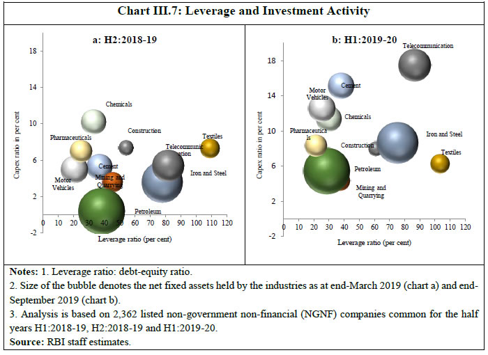 As per the first revised estimates, gross domestic saving (GDS) rate decreased to 30.1 per cent of GDP in 2018-19 from 32.4 per cent in 2017-18. The saving rate of the household sector, which is a net supplier of funds to the economy, declined from 23.6 per cent of GDP in 2011-12 to 18.2 per cent in 2018-19. While the private corporate sector finances its investment predominantly through its own savings, the public sector continues to rely heavily on households for financing its deficit (Chart III.8). During April-December 2019, household financial savings appeared to have improved as households’ liabilities declined more than the increase in household deposits with scheduled commercial banks whereas their investment in insurance and mutual funds remained at the same level as in the previous year. III.1.3 Government Expenditure Growth in government final consumption expenditure (GFCE) moderated in H2:2019-20 due to a sharp slowdown in Q4 as implicit in the SAE released by the NSO. During January-February 2020, revenue expenditure of the Centre grew by 3.9 per cent. In 2020-21, revenue expenditure is budgeted higher than in 2019-20 revised estimates (RE) (Table III.2). | Table III.2: Key Fiscal Indicators – Central Government Finances | | Indicator | Per cent to GDP | | 2019-20 (BE) | 2019-20 (RE) | 2020-21 (BE) | | 1. Revenue Receipts | 9.3 | 9.1 | 9.0 | | a. Tax Revenue (Net) | 7.8 | 7.4 | 7.3 | | b. Non-Tax Revenue | 1.5 | 1.7 | 1.7 | | 2. Non-Debt Capital Receipts | 0.6 | 0.4 | 1.0 | | 3. Revenue Expenditure | 11.6 | 11.5 | 11.7 | | 4. Capital Expenditure | 1.6 | 1.7 | 1.8 | | 5. Total Expenditure | 13.2 | 13.2 | 13.5 | | 6. Gross Fiscal Deficit | 3.3 | 3.8 | 3.5 | | 7. Revenue Deficit | 2.3 | 2.4 | 2.7 | | 8. Primary Deficit | 0.2 | 0.7 | 0.4 | Note: BE: Budget Estimates. RE: Revised Estimates.
Source: Union Budget, 2020-21. | During 2019-20 (April-February), the fiscal position of the central government deteriorated mainly due to a decline in gross revenue under corporation tax, reflecting mid-year cut in tax rates. GST collections at ₹5.5 lakh crore were 89.5 per cent of RE and 4.5 per cent higher than a year ago. On the whole, direct taxes contracted by 3.3 per cent, while indirect taxes grew barely by 1.6 per cent in the first 11 months of the year, lower than the budget estimates (BE) (Chart III.9 a & b). Revenue expenditure growth also stood lower than the RE mainly due to lower interest payments. Outgoes on account of major subsidies moderated from the BE of 1.4 per cent of GDP to 1.1 per cent in RE due to curtailment of on-budget food subsidy. Nonetheless, food subsidy continues to dominate the overall subsidy bill. Capital expenditure growth was also lower than in the RE. Under the provisions of section 4(3) of the revised FRBM Act, which can be invoked under specific conditions4, the Centre’s GFD was revised up to 3.8 per cent of GDP in 2019-20 (RE) from the budgeted 3.3 per cent, due to a shortfall in tax revenue and disinvestment proceeds. The implications of these evolving dynamics can be examined in a general equilibrium framework (Box III.3). The GFD is budgeted to moderate to 3.5 per cent of GDP in 2020-21 and in a glide path it will return to 3.1 per cent by 2022-23. Based on the latest available data, the gross fiscal deficit of 22 states increased to 2.9 per cent of their gross state domestic product (GSDP) in 2019-20 (RE) from the budgeted 2.5 per cent (Table III.3). The deviation was mainly caused by lower revenue – both own and central transfer – due to the slowdown in economic activity, which, in turn, induced states to cut both revenue and capital expenditure in an adverse feedback loop that further weakened aggregate demand. For 2020-21, states have budgeted a consolidated GFD of 2.4 per cent of GSDP, anticipating higher revenue and lower expenditure than a year ago. | Table III.3: State Government Finances - Key Deficit Indicators | | (per cent to GSDP) | | Item | 2018-19 | 2019-20 (BE) | 2019-20 (RE) | 2020-21 (BE) | | Revenue Deficit | 0.1 | 0.1 | 0.7 | 0 | | Gross Fiscal deficit | 2.4 | 2.5 | 2.9 | 2.4 | Notes: 1. Negative (-) sign indicates surplus.
2. Data pertain to 22 out of 28 States.
3. GSDP is the sum of GSDP of respective 22 states.
Sources: Budget Documents of State Governments. | Under the centre’s market borrowing programme during 2019-20, that is managed by the Reserve Bank, gross borrowings were ₹2,68,000 crore during H2:2019-20, as compared to ₹2,83,000 crore during H2:2018-19, i.e., lower by 5.3 per cent than their level a year ago. Net market borrowings during H2:2019-20 at ₹1,33,000 crore were also 43.2 per cent lower. As part of active debt consolidation, seven tranches of switch operations worth ₹1,24,694 crore were carried out during H2:2019-20 with the objective of managing redemption and enhancing liquidity of government securities. Furthermore, cash management bills worth ₹2,50,000 crore were issued on seven occasions during H2:2019-20 to tide over frequent recourse to ways and means advances/overdrafts in the face of negative cash balances with the Reserve Bank. States completed their gross borrowings of ₹6,34,521 crore for the year (Table III.4). | Table III.4: Government Market Borrowings | | (₹ crore) | | Item | 2017-18 | 2018-19 | 2019-20 | | Centre | States | Total | Centre | States | Total | Centre | States | Total | | Net Borrowings | 4,48,410 | 3,40,281 | 7,88,691 | 4,22,737 | 3,48,643 | 7,71,380 | 4,73,972 | 4,87,454 | 9,61,426 | | Gross Borrowings | 5,88,000 | 4,19,100 | 10,07,100 | 5,71,000 | 4,78,323 | 10,49,323 | 7,10,000 | 6,34,521 | 13,44,521 | | Sources: Government of India; and RBI staff estimates. |
Box III.3 Augmenting Quarterly Projection Model (QPM): Fiscal Block Fiscal policy measures can impact output, inflation and monetary policy decisions and vice versa (Government of India, 2017). However, all fiscal measures need not affect the macroeconomic variables in a similar way. The various conduits of fiscal-monetary interface and their impact on growth and inflation are assessed by incorporating a fiscal block in RBI’s Quarterly Projection Model (QPM)5. Salient features of the fiscal block in the QPM are the following: (a) headline fiscal deficit is decomposed into structural and cyclical primary deficits and interest payments; (b) the cyclical component of the primary deficit depends on the state of the economy and recognises that government tax revenue will be lower and expenditure will be higher leading to higher fiscal deficit when the overall economy slows down and vice versa; (c) deviation of the fiscal deficit from the announced fiscal path on account of cyclically-adjusted (i.e., structural – the part of fiscal deficit which is not related to the state of the economy) component of the primary deficit is a fiscal impulse and contributes to aggregate demand; (d) link between debt dynamics and fiscal deficit is identified for stock-flow consistency (Escolano, 2010); (e) the fiscal deficit and debt has implications for the country risk premium and the exchange rate; and (f) monetary policy’s interaction with the fiscal deficit is captured through interest payments (Chart III.3.1). 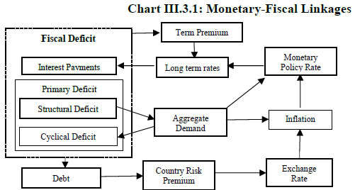 The model’s dynamics indicate that a shock to the cyclically-adjusted (structural) fiscal deficit impacts aggregate demand. The higher level of debt to finance higher fiscal deficit leads to increase in country risk premium and exchange rate depreciation. Thus, inflation gets impacted through both the aggregate demand and exchange rate channels. However, if the deviation of the headline fiscal position from the announced path is on account of cyclical factors, the impact on inflation and output would be muted (Chart III.3.2). 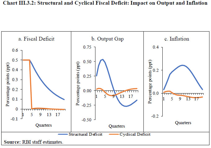 In 2019-20, the GDP growth has slowed down, which contributed to an increase in the fiscal deficit mainly on account of (a) lower aggregate demand (denominator), (b) lower fiscal revenue due to lower economic activity, and (c) higher fiscal expenditure on account of the measures to address the economic slowdown. Thus, a considerable portion of the fiscal deficit deviation in 2019-20 could be attributed to cyclical factors. In such scenario, the inflationary impact of this deviation was largely subdued. References: Escolano, M. J. (2010), “A Practical Guide to Public Debt Dynamics, Fiscal Sustainability, and Cyclical Adjustment of Budgetary Aggregates”, Technical Notes and Manuals 10/02, International Monetary Fund. Government of India (2017), “Fiscal Responsibility and Budget Management Review Committee” (Chairman: N.K Singh). | III.1.4 External Demand Net exports contributed positively to aggregate demand in H2:2019-20, with imports contracting more sharply than exports (Chart 10). According to data released by the Directorate General of Commercial Intelligence and Statistics (DGCI&S), the contraction in merchandise exports, which started in Q1:2019-20, accentuated in Q2, as the slump in shipment of engineering goods, gems and jewellery, cotton and handloom products, and rice became pronounced in the face of a prolonged slowdown in world trade and demand. The pace of overall export contraction moderated during Q3:2019-20, and eventually there was a turnaround in February, supported by petroleum, oil and lubricants (POL), engineering goods, electronic goods and chemicals (Chart III.11a). Overall, exports shrank by 1.5 per cent during April-February 2019-20, though the adverse impact of COVID-19 on global supply chains and global economic activity more generally may dent export performance in March. 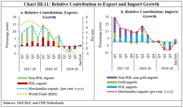 Imports contracted in Q2:2019-20, pulled down by gold, POL and non-POL non-gold imports (Chart III.11b). Within the latter, the decline was broad-based and covered sectors such as transport equipment, pearls and precious stones, coal and chemicals. Imports also contracted in Q3 and in January 2020, but expanded in February, driven by POL, pearls and precious stones and machinery. Overall, imports contracted by 7.3 per cent during April-February 2019-20. With imports declining more than exports, the trade deficit narrowed from US$ 173.0 billion in April-February 2018-19 to US$ 143.1 billion in April-February 2019-20. India’s oil import bill is expected to decline in March with a steep fall in crude oil prices and this may compress the trade deficit further for the full year. The current account deficit (CAD) narrowed to 0.2 per cent of GDP in Q3:2019-20 from 0.9 per cent in Q2:2019-20 and from 2.7 per cent in Q3 a year ago. The contraction in the CAD was primarily on account of a lower trade deficit and a rise in net services receipts. Services exports grew on the back of a rise in net earnings from software, travel and financial services (Chart 10.b). Remittances from overseas Indians were strong in Q3:2019-20, while the net outgo of payments due to investment income and compensation of employees together, remained broadly unchanged from the previous year. Net capital inflows exceeded the CAD in Q3:2019-20. Net foreign direct investment (FDI) flows at US$ 37.8 billion in April-January 2019-20 were higher than those a year ago, flowing mainly to manufacturing, communication, retail and wholesale trade, financial and computer services. Amidst growing risk aversion on fears of global recession in the wake of COVID-19 pandemic, foreign portfolio investors (FPIs) turned net sellers beginning February 18, 2020. Foreign portfolio investment (FPI) outflows accentuated further from March 6, 2020 as the oil price war between Saudi Arabia and Russia caused fresh turbulence in global financial markets. Overall, FPI outflows were of the order of US$ 7.1 billion in 2019-20 (up to March 31, 2020). Under the voluntary retention route, however, net investment by FPIs amounted to US$ 8.7 billion up to March 31, 2020. Net disbursals under external commercial borrowings (ECBs) by Indian entities at US$ 3.2 billion in Q3:2019-20 were higher than those of US$ 2.0 billion a year ago. Net International Investment Position (IIP), i.e., the difference between a country’s external financial assets and liabilities, improved during Q3:2019-20 over Q2. India’s foreign exchange reserves were placed at US$ 475.6 billion, equivalent to 11.8 months of import, as on March 27, 2020 – an increase of US$ 62.7 billion over the level at end-March 2019. III.2 Aggregate Supply Gross value added (GVA) growth at basic prices – the metric for aggregate supply – decelerated to 4.7 per cent in H2:2019-20 from 5.1 per cent in H1 and 5.6 per cent in H2:2018-19 (Table III.5). This deceleration can be attributed to base effects to a large extent since its momentum measured in terms of q-o-q SAAR accelerated to 5.6 per cent in H2 from 4.2 per cent in H1 (Chart III.12a). With COVID-19 impacting the GVA in the last phase of Q4 strongly, it is unlikely that this momentum would be maintained as the year closed. The slowdown in y-o-y GVA growth reflected the deceleration in industrial and services activities. On the other hand, GVA growth in agriculture and allied activities accelerated in H2:2019-20 in comparison with both H1:2019-20 and H2:2018-19, buoyed by the late surge in south-west monsoon rainfall and bountiful north-east monsoon precipitation. Based on the Ministry of Agriculture & Farmers Welfare’s second advance estimates, production of all major food grains, except urad and moong, in 2019-20 was higher than the final estimates of the preceding year. Public administration, defence and other services (PADO) continued to provide support to overall supply conditions (Chart 12b). | Table III.5: Sector-wise Growth in GVA | | (y-o-y, per cent) | | Sector | 2018-19
(FRE) | 2019-20
(SAE) | Weighted | 2018-19 (FRE) | 2019-20 (SAE) | | 2019-20 | Q1 | Q2 | Q3 | Q4 | Q1 | Q2 | Q3 | Q4# | | Agriculture, forestry and fishing | 2.4 | 3.7 | 0.5 | 3.8 | 2.5 | 2.0 | 1.6 | 2.8 | 3.1 | 3.5 | 5.0 | | Industry | 4.5 | 1.5 | 0.3 | 7.8 | 4.7 | 4.4 | 1.4 | 3.2 | 0.1 | 0.1 | 2.3 | | Mining and quarrying | -5.8 | 2.8 | 0.1 | -7.3 | -7.0 | -4.4 | -4.8 | 4.7 | 0.2 | 3.2 | 2.6 | | Manufacturing | 5.7 | 0.9 | 0.2 | 10.7 | 5.6 | 5.2 | 2.1 | 2.2 | -0.4 | -0.2 | 1.8 | | Electricity, gas, water supply and other utilities | 8.2 | 4.6 | 0.1 | 7.9 | 9.9 | 9.5 | 5.5 | 8.8 | 3.9 | -0.7 | 6.5 | | Services | 7.5 | 6.5 | 4.1 | 7.3 | 7.2 | 7.3 | 8.3 | 6.7 | 6.8 | 6.4 | 6.1 | | Construction | 6.1 | 3.0 | 0.2 | 6.4 | 5.2 | 6.6 | 6.0 | 5.5 | 2.9 | 0.3 | 3.2 | | Trade, hotels, transport, communication | 7.7 | 5.6 | 1.1 | 8.5 | 7.8 | 7.8 | 6.9 | 5.7 | 5.8 | 5.9 | 5.1 | | Financial, real estate and professional services | 6.8 | 7.3 | 1.6 | 6.0 | 6.5 | 6.5 | 8.7 | 6.9 | 7.1 | 7.3 | 8.0 | | Public administration, defence and other services | 9.4 | 8.8 | 1.1 | 8.8 | 8.9 | 8.1 | 11.6 | 8.7 | 10.1 | 9.7 | 6.7 | | GVA at Basic Prices | 6.0 | 4.9 | 4.9 | 6.9 | 6.1 | 5.6 | 5.6 | 5.4 | 4.8 | 4.5 | 5.0 | FRE: First Revised Estimates; SAE: Second Advance Estimates. #: Implicit growth.
Source: NSO. |
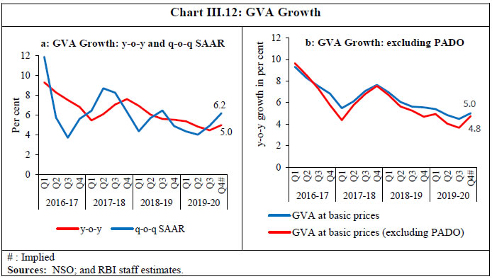 III.2.1 Agriculture GVA growth at basic prices in agriculture and allied activities accelerated in H2:2019-20 to 4.2 per cent from 3.0 per cent in H1:2019-20. Acreage of rabi crops increased by 9.5 per cent, underpinned by the favourable northeast monsoon, sufficient reservoir levels, improved soil moisture and an increase in prices for agricultural commodities. The second advance estimates of crop production for 2019-20 placed kharif and rabi foodgrain production higher by 0.6 and 4.1 per cent, respectively (Table III.6). Horticultural production was placed at a record level of 3,133.5 lakh tonnes during 2019-20, 0.8 per cent higher than the final estimates for 2018-19 and driven largely by production of vegetables. | Table III.6: Agricultural Production in 2019-20 (Second Advance Estimates) | | (in Lakh Tonnes) | | Crop | 2018-19 | 2019-20 | 2019-20 Variation (Per cent) | | 2nd AE | Final | Target | 2nd AE | Over 2nd AE 2018-19 | Over Final 2018-19 | Over Target | | Foodgrains | 2814 | 2852 | 2911 | 2920 | 3.8 | 2.4 | 0.3 | | Rice | 1156 | 1165 | 1160 | 1175 | 1.6 | 0.8 | 1.3 | | Wheat | 991 | 1036 | 1005 | 1062 | 7.2 | 2.5 | 5.7 | | Pulses | 240 | 221 | 263 | 230 | -4.2 | 4.3 | -12.5 | | Oilseeds | 315 | 315 | 361 | 342 | 8.5 | 8.5 | -5.3 | | Sugarcane | 3808 | 4054 | 3855 | 3538 | -7.1 | -12.7 | -8.2 | | Cotton # | 301 | 280 | 358 | 349 | 16 | 24.4 | -2.4 | | Jute & Mesta ## | 101 | 98 | 112 | 98 | -2.6 | -0.1 | -12.4 | #: Lakh bales of 170 kgs. each.
##: Lakh bales of 180 kgs. each.
Source: Ministry of Agriculture and Farmers’ Welfare, Government of India. | Allied activities, including livestock, forestry and fishing, constitute about 40 per cent of the GVA in agriculture and allied sector and contributed four-fifths of overall agricultural GVA growth during 2012-19 (Chart III.13). According to the US National Oceanic and Atmospheric Administration (NOAA), near- to above-average sea surface temperatures (SSTs) prevailed across the equatorial Pacific Ocean during March 2020. There is 65 per cent chance of ENSO6-neutral prevailing in the spring and 55 per cent chance in the summer of 2020. The Australian Bureau of Meteorology (BoM) has indicated that the ENSO Outlook is neutral, suggesting low or no possibility of El Niño or La Niña developing in the coming months. Skymet expects neutral conditions to prevail during monsoon months with more than 50 per cent probability. The India Meteorological Department also expects ENSO-neutral conditions to prevail during April-June 2020. III.2.2 Industrial Sector In the industrial sector, GVA growth at basic prices decelerated to 1.3 per cent in H2:2019-20 from 1.7 per cent in the preceding half, and 2.8 per cent a year ago (Chart III.14). It was the deceleration in the manufacturing sector – the dominant component of industry – that deepened this slowdown, due to weak domestic and external demand. The mining sector growth picked up, but electricity generation weakened. Among the high frequency indicators, the index of industrial production (IIP) emerged out of contraction in November 2019 and remained in positive territory in the following two months. The truncated IIP, by taking 96 per cent of IIP, i.e., excluding top 2 per cent and bottom 2 per cent of volatile items, improved marginally in January 2020 (Chart III.15a). Manufacturing IIP contracted in Q3:2019-20, pulled down by a decline in the production of motor vehicles, machinery and equipment, computer, electronic and optical products, fabricated metal products, rubber and plastics products. Of the 23 industry groups constituting the IIP, 17 contracted during Q3 as against 15 during Q2. In terms of the use-based classification, the intermediate goods sector grew by double digits in Q3:2019-20 led by growth in mild steel (MS) slabs. On the other hand, consumer non-durables slipped into contraction (Chart III.15b). Primary goods, infrastructure and consumer durables remained in contraction in Q3. The consumer durables segment contracted in Q3:2019-20 due to the decline in production of two wheelers, TV sets and auto components. The capital goods sector also remained in contraction in Q3 mainly due to weak investment demand pertaining especially to commercial vehicles and power generation. In January 2020, while the IIP growth was positive at 2.0 per cent, this was also broad-based. However, its sustainability in the near term seems to be uncertain in view of supply chain disruptions caused by COVID-19 and weak automobile sales. Intermediate goods continued to register robust growth emanating mostly from mild steel slabs, which contributed 197 basis points to headline IIP growth in January. Capital goods production continued to contract, taking the sequential decline to its thirteenth consecutive month. 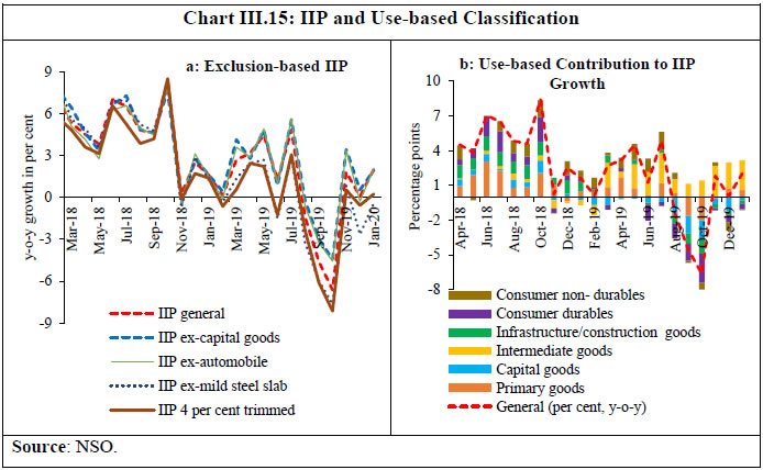 Electricity generation decelerated in H2 in comparison with H1, reflective of low demand from the organised manufacturing sector amidst extended monsoon season. This subdued performance was mainly on account of thermal power generation, the source of two-thirds of energy supply. Electricity generation increased in December-January 2020, after six months of contraction (Chart III.16). In the mining sector, production picked up marginally in H2 but remained weak. Recent announcements by the Government such as doing away with end-use restrictions in coal mining, extending the validity of clearances for mining leases and opening up of this sector to new participants may spur activity in this sector. 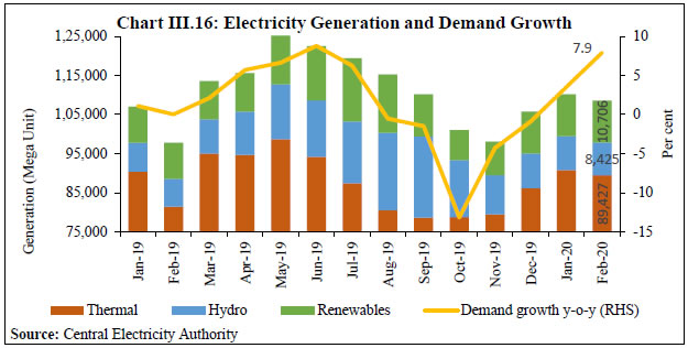 The Reserve Bank’s business assessment of the industrial outlook survey (IOS)7 showed improvement in Q4:2019-20, with the sentiment on employment conditions slightly improved. In view of the intensification of COVID-19, a quick survey with select parameters was specially conducted during March 18-20 to capture the updated sentiments of the enterprises. The limited responses received indicate a considerable worsening of the key demand indicators in Q4:2019-20 and the pessimism was more pronounced in the outlook for the next quarter. Manufacturing PMI softened to 51.8 in March from 54.5 in February due to the marked decline in new business order (export); the COVID-19 negatively impacted the supply-side of the sector, with suppliers' delivery times lengthening for the first time in five months. Services PMI moved to contraction zone: 49.3 in March from a seven-year high of 57.5 in February due to deterioration in new export business as well as business expectations. III.2.3 Services Service sector activity moderated in H2:2019-20, pulled down by a slowdown in construction and trade, hotels, transport and communication and PADO (Chart III.17a). The slowdown in the construction sector was reflected in a decline in one of its key indicators, viz., cement production (Chart III.17b). Growth in trade, hotels, transport, communication and services related to broadcasting was muted in H2:2019-20. Commercial vehicle sales – a lead indicator for road transport – continued to contract in H2:2019-20 as the impact of the upward revision in axle norms8 in July 2018 lingered (Chart III.18a). Other constituents of the transport segment like freight traffic by rail, water and air improved marginally in December-February 2019-20 (Chart III.18b). The growth of financial, real estate and professional services accelerated in H2:2019-20, reflecting the robust performance of information technology companies in the professional services segment. However, the growth of aggregate deposits and bank credit remained muted (Chart III.19). The growth of public administration, defence and other services (PADO) moderated in Q3:2019-20, reflecting subdued revenue expenditure (net of interest payments and subsidies) of the Union and the state governments. This has likely got accentuated in Q4 in view of the tight financial position of the Centre and States: the Union finance ministry has directed all government departments and ministries to restrict their expenditures within the budgeted level. The residential real estate sector has continued to suffer from low demand and large inventory overhang. As a result, new launches declined in Q3:2019-20 (Chart III.20a). Reflecting the large volume of inventory overhang, all-India level housing prices have moderated somewhat (Chart III.20b). III.3 Output Gap The output gap – the deviation of actual output from its potential level and expressed as a proportion to potential output – is a summary measure of demand-supply conditions in the economy and an important input for monetary policy formulation, since it provides a ‘fix’ about the position of the economy vis-à-vis the underlying business cycle. As potential output is unobservable, it has to be empirically estimated and hence, it is sensitive to the choice of methodology, time period and revisions in data. A variety of measures - univariate filters such as the Hodrick-Prescott (HP) filter, the Baxter-King (BK) filter and the Christiano-Fitzgerald (CF) filter and the multivariate Kalman filter (MVKF) taking into account inflation developments – are used to assess the state of business cycle. The composite estimate, by combining all these measures, suggests that the output gap was negative in Q3:2019-20 (Chart III.21). III.4 Conclusion In Q3:2019-20, the economy hit a multi-quarter low and going forward, the risks are tilted largely to the downside. Private consumption, in particular, is at serious risk from the COVID-19 pandemic, notwithstanding improved rabi prospects and the recent rise in food prices, and the rationalisation of personal income tax rates in the Union Budget 2020-21 along with measures to boost rural and infrastructure spending. Aggregate demand is expected to be impacted adversely by likely recession in the global economy, caused by disruptions in global supply chains, travel and tourism, and lockdowns in many economies. Domestic production will also be impacted by the nation-wide lockdown. In the near-term, the challenge is to mitigate the adverse impact of COVID-19. _____________________________________________________________________________
IV. Financial Markets and Liquidity Conditions Domestic financial markets were overwhelmingly influenced by evolving domestic and global developments and the outbreak of COVID-19 in India in end-January 2020. Markets witnessed heightened volatility beginning February, culminating into a state of seizure in March with a sharp shrinkage in trading activity. Search for safe haven assets and flight to safety resulted in large scale capital outflows which sent equity markets into a tailspin and exerted sharp depreciation pressure on the Indian Rupee. The risk premium in the bond markets increased sharply amidst increasing fears of illiquidity. Global financial markets turned volatile during the latter part of H2:2019-20 against the backdrop of geo-political tensions between Iran and the US and outbreak of the coronavirus (COVID-19) pandemic, the latter overwhelming the positive impact of de-escalation of trade tensions between the US and China and the UK election outcome being conducive to an amicable resolution of Brexit. Towards end-February and early-March, global markets experienced episodic meltdowns as COVID-19 spread out of China to many countries rapidly. The severity of the crisis prompted emergency rate cuts by the US Federal Reserve on March 3 and March 15, 2020. Similar moves by the central banks in Canada, the UK, Australia, New Zealand and several others were backed up by measures, both conventional and unconventional to unfreeze markets, ensure adequate liquidity and ease financial conditions. Amidst heightened uncertainty, equity markets in many advanced economies (AEs) and emerging market economies (EMEs) suffered their worst week after the global financial crisis (GFC) during March 9-16, 2020. Bond yields fell sharply, most noticeably in the US where the 10- year benchmark yield fell below 1 per cent on the days of the Fed rate cut on March 03 and March 15. In currency markets, the US dollar appreciated in December as trade tensions receded and gained further on safe haven demand after the COVID-19 outbreak. Most EME currencies weakened sharply with flight to safety intensifying in late February and early March. IV.1 Domestic Financial Markets During H2:2019-20, domestic financial markets exhibited divergent movements. A policy rate cut in October 2019 and liquidity management operations undertaken by the Reserve Bank of India (RBI) enthused market sentiment but growing concerns about the domestic economic slowdown, fiscal slippages, geo-political tensions and heightened uncertainties caused by the rapid spread of COVID-19 posed significant challenges, particularly towards the close of Q4. An unscheduled meeting of the Monetary Policy Committee (MPC) of the RBI on March 24, 26 and 27 delivered an unprecedented reduction in the policy repo rate and the announcement of several liquidity-augmenting measures briefly assuaged market fears (see Box IV.3). In the credit market, monetary policy transmission was facilitated by large surplus liquidity, long term repo operations (LTROs) targeted to reduce banks’ cost of funds, simultaneous purchase and sale of securities under open market operations (special OMOs)1 and exemption from cash reserve ratio (CRR) requirements to incentivise lending to specific sectors. Equity markets scaled a new high on January 14, 2020, but turned highly volatile thereafter in sync with global markets. The Indian Rupee (INR) came under pressure due to fears sparked by the spread of pandemic and flight to safety. In the event, however, the depreciation of INR was significantly lower than currencies of many EME peers. IV.1.1 Money Market Money markets have remained broadly resilient reflecting the RBI’s proactive liquidity management operations. During H2, the weighted average call rate (WACR) in the unsecured overnight money market has remained within the policy corridor with a downward bias (13 bps below the repo rate on an average basis) reflecting sustained surplus liquidity (Chart IV.1). The WACR spiked in the typical financial year-end phenomenon, compounded by reduced market participation because of the COVID-19 induced nation-wide lockdown. In the overnight call money segment, the weighted average rate of traded deals continued to be higher than that of reported deals.2 The share of traded deals (in terms of volume) was also higher vis-a-vis reported deals, though the latter picked up in H2 vis-à-vis H1 on: (i) increased lending by co-operative banks; and (ii) higher levels of surplus liquidity in the second half of the year (Chart IV.2). The share of the collateralised money market (triparty repo and market repo) in the overnight money market volume increased in H2:2019-20 (Chart IV.3). The dependency of banks on the call money market, however, has increased (the share of call money in total overnight transactions increased to 6 per cent during February-March 2020 from 4 per cent in January), partly reflecting the discontinuation of the daily fixed rate repo operations since February 14, 2020 as part of the revised liquidity management framework announced on February 06, 2020 (see Box IV.2). 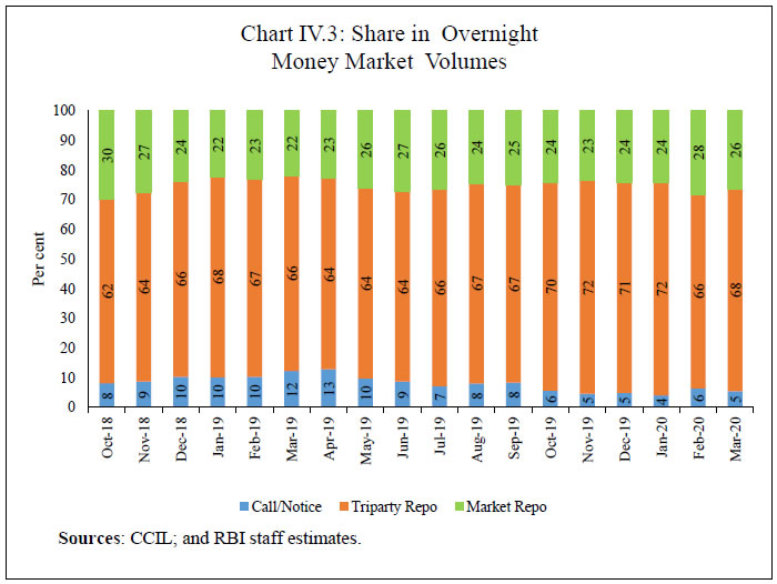 In particular, the share of triparty repo in overnight money market volumes improved due to increased lending by mutual funds (MFs) from October 2019. The change in the cut-off timing3 for applicability of net asset value (NAV) on purchase of units in liquid and overnight funds has given more leeway to asset management companies (AMCs) to deploy funds in the triparty repo segment. Accordingly, the share of lending by MFs in triparty repo increased from 60.5 per cent in September 2019 to 64.7 per cent in October and peaked at 72.1 per cent in March. Concomitantly, borrowings by MFs reduced sharply from 9.8 per cent in September 2019 to 2.4 per cent in October, averaging only 2.2 per cent in the succeeding months. During H2:2019-20, interest rates in the collateralised overnight money market segments softened in tandem with the WACR, though the moderation was more pronounced around the time of the conduct of the third auction of the special OMOs on January 06, 2020. Overnight rates in the triparty repo and market repo segments declined sharply towards end-March 2020, with the former trading close to zero as liquidity surplus increased in the wake of extreme risk-aversion gripping investors, including corporates and non-banks. The triparty repo and market repo traded below the WACR (on an average) by 36 bps and 37 bps, respectively, in H2. Interest rates on longer-term money market instruments such as certificates of deposit (CDs), commercial paper (CPs) and treasury bills (T-Bills) of 3-month maturity moved divergently, responding to the policy rate cut in October and the build-up of surplus liquidity (Chart IV.4). CP rates experienced intermittent bouts of volatility before hardening in late-February and early-March 2020.  In view of the persistent liquidity surplus, banks reduced their recourse to CDs as fresh issuances declined to ₹1,86,954 crore during H2:2019-20 from ₹2,01,302 crore during H1. CP issuances also declined to ₹10,02,667 crore in H2 from ₹12,38,324 crore in H2:2018-19, mainly reflecting risk aversion. The weighted average discount rate (WADR) of CPs in the primary market generally eased up to February (i) in sync with the build-up of surplus liquidity; and (ii) with the predominance of issuances by top rated issuers backed by relatively stronger parent companies. The WADR, which had firmed up by 24 bps in December 2019 reflecting credit rating concerns, increased sharply by 229 bps in March on account of contagion fears arising out of (i) COVID-19 induced financial stress; and (ii) interconnectedness in the banking system with distress in a private sector bank (Chart IV.5a). The share of non-banking financial companies (NBFCs) in primary issuances of CPs, which had declined immediately after the IL&FS crisis, increased in October subsequently peaking at around 35 per cent in March 2020 (Chart IV.5b). 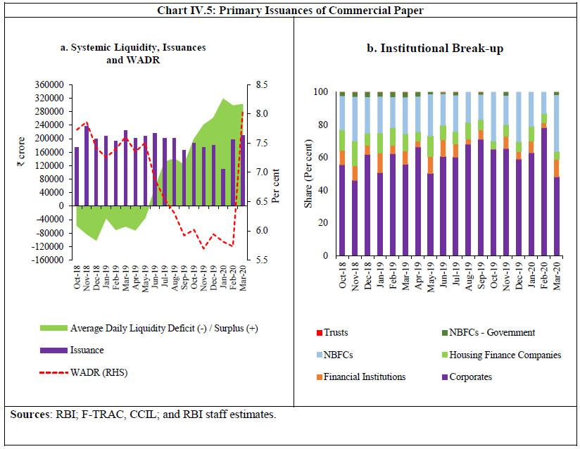 Monetary policy transmission was more than proportionate in the triparty repo and market repo segments, facilitated by large surplus liquidity conditions in H2:2019-20 and partly due to the year-end phenomenon as discussed earlier (Table IV.1). The risk premium (on an average) in the money market (3-month CPs over 91-day T-Bills), however, firmed up to 97 bps in H2 from 87 bps in H1, driven by fears of illiquidity and market seizure post COVID-19 induced turbulence in global and domestic financial markets. | Table IV.1: Policy Transmission in the Money Market | | (basis points) | | Changes in rate | | 2019-20 | Repo | Call/Notice (WACR) | Triparty Repo | Market Repo | 3-Month CD | 91-Day T-Bill | 3-Month CP | | H1: (April 02 – Sep 30) | -85 | -162 | -111 | -178 | -132 | -90 | -59 | | H2: (Oct 01 – Mar 31) | -100 | -111 | -477 | -416 | -94 | -100 | -100 | Note: easing (-) / hardening (+).
Sources: RBI; CCIL; F-TRAC, CCIL; FBIL; and RBI staff estimates. | IV.1.2 Government Securities (G-sec) Market At the beginning of H2:2019-20, the benchmark G-sec yield softened by 4 bps on (i) market expectations of monetary policy easing; (ii) the Centre’s decision to announce the auction of a new 10-year paper; and (iii) a benign inflation trajectory. Yields, however, firmed up by 8 bps after the policy announcement on October 4, 2019 as the rate cut of 25 bps fell short of market expectations. Yields continued to harden thereafter due to persistent worries about the Centre's finances, expectation of a rise in inflation prints and subdued appetite for government paper. They moderated towards end-October, however, taking cues from (i) a decline in the overnight index swap (OIS) rates; (ii) a fall in global crude oil prices; and (iii) softening of US treasury yields. Overall, the benchmark yield declined by 5 bps during October 2019. Yields firmed up by 7 bps on both the new benchmark (6.45% GS 2029) and the old benchmark (7.26% GS 2029) as on November 5, 2019 reflecting concerns about fiscal slippages, and the hardening of US treasury yields. At the beginning of December, both benchmark yields increased due to market sentiment turning jittery about the Centre’s fiscal position. On the day of the monetary policy announcement on December 5, yields hardened by 14 bps on the new benchmark and by 18 bps on the old benchmark in the wake of (i) the MPC’s decision to keep the policy rate unchanged in the face of upside risks to inflation; and (ii) foreign portfolio investors (FPIs) selling heavily on a pessimistic growth outlook. Market participants, however, welcomed the Reserve Bank’s decision to conduct special OMOs on December 19, which resulted in new and old benchmark yields shedding 15 bps and 13 bps, respectively.4 Yields softened at the long end, while firming up at the short-end, thereby reducing the term premium (Box IV.1). On the whole, the new and the old benchmark yields increased by 9 bps and 15 bps, respectively, in December. Box IV.1: Estimating Term Premium and its Determinants The term premium is the difference in yield of a long-term bond vis-a-vis a short-term bond and reflects the excess return investors demand for holding bonds of longer maturity (Swanson, 2007). The long-term interest rates at any maturity can be decomposed into two components: (i) risk-neutral rate that reflects expectations of future short-term rates; and (ii) term premium, which is indicative of investors’ expectations relating to future central bank policy, inflation and growth outlook, given the expected future path of short-term interest rates. The Adrian, Crump and Moench (ACM) approach, which allows for the decomposition of yield into risk-neutral component and term premium, belongs to the regular class of dynamic term structure models (Adrian et al., 2013). These models are premised on the no-arbitrage condition5. The ACM approach uses principal components of bond yields as pricing factors. The risk-neutral rate is modelled as a linear function of these pricing factors. The longer-term yields are also obtained as linear functions of the pricing factors, with appropriate restrictions on parameters to incorporate the assumptions of the no-arbitrage, affine term-structure models. The time-varying term premium is the difference between the model-fitted yield and the risk- neutral yield. Decomposition Empirical analysis in the Indian context involves decomposition of 10-year government bond yield into expectation and term premium components following the ACM methodology (Dilip, 2019), based on monthly data on 10-year G-sec yields spanning April 2009 to February 2020. This shows that the 10-year yield has broadly tracked movements in the term premium (Chart IV.1.1).
| Table IV.1.1: Share of Term Premium in Bond Yield Variations | | (per cent) | | Tenor | India | US | | 1-years | 26.7 | 41.4 | | 2-years | 38.8 | 45.0 | | 3-years | 50.4 | 49.8 | | 4-years | 58.5 | 53.3 | | 5-years | 64.1 | 55.9 | | 6-years | 70.2 | 58.1 | | 7-years | 74.7 | 60.1 | | 8-years | 78.1 | 61.9 | | 9 years | 81.6 | 63.7 | | 10 years | 84.4 | 65.4 | | Source: RBI staff estimates. | In order to identify the determinants of the term premium in India, the 10-year term premium is regressed on its own lag, G-Sec market depth proxied by daily average turnover as proportion of GDP, international oil prices, the INR-USD spot exchange rate, systemic liquidity measured by outstanding balances under the liquidity adjustment facility as proportion of GDP , and both global and India-specific policy uncertainty represented by Global Economic Policy Uncertainty Index (GEPU) and Economic Policy Uncertainty (EPU) for India, respectively. The differenced series of all the explanatory variables is found to be stationary and the equation is estimated in an ordinary least squares (OLS) framework. Most of the estimated coefficients are statistically significant with expected signs (Table IV.1.2). The high coefficient of the lagged term indicates persistence of the term premium. The significance of the turnover and systemic liquidity variables is indicative of the important role of liquidity in higher demand for bonds and a consequent reduction in term premium. Movements in oil prices and the exchange rate of Indian Rupee (INR) also impact yields significantly – a spike in oil prices and a depreciation of the INR leads to search for safe haven assets among investors, resulting in flight to safety (panic selling) and increase in term premium. Global uncertainty (lagged) and Indian policy uncertainty, although having a positive impact, are not statistically significant. | Table IV.1.2: Determinants of Term Premium | | Variable | Coefficient | | Term_Premium (-1) | 0.83 *** (9.60) | | ΔAverage_Turnover | -5.35*** (-5.57) | | Δ(Crude_Oil_Price) | 0.02***(6.65) | | Δ(INR/USD) | 0.08*** (3.33) | | Δ(Systemic_Liquidity) | -0.89**(-2.14) | | Δ (Global_ Uncertainty)(-1) | 0.003(0.77) | | Δ(Policy_Uncertainty) | 0.001(0.81) | | c | 0.29* (1.76) | | R-bar2 | 0.82 | | Durbin Watson | 1.64 | | LB-Q (p-value) | 0.59 | ***, **, * represent significance at 1%, 5% and 10% levels, respectively
Note: Figures in parentheses are t-statistics based on heteroscedasticity and autocorrelation consistent (HAC)-corrected standard errors; LB-Q is p-value of Box-Pierce-Ljung Q-statistic for the null hypothesis of no correlation up to 4 lags; and Δ is the difference operator.
Average_Turnover = Daily average turnover (% of GDP), Crude_Oil_Price = Price of Brent Crude Oil in USD/barrel, INR/USD= Spot Rupee-US Dollar exchange rate, Systemic_Liquidity = Outstanding LAF balance (% of GDP), Global_ Uncertainty = Global Economic Policy Uncertainty Index (GEPU), Policy_Uncertainty = Economic Policy Uncertainty (EPU) for India.
Source: RBI staff estimates. | References: Adrian, T., Crump, R. K., & Moench, E. (2013), “Pricing the term structure with linear regressions”, Journal of Financial Economics, 110(1), 110-138. Dilip, A. (2019), “Term premium spillover from the US to Indian markets”, RBI Working Paper Series, WPS (DEPR): 05 / 2019, December. Swanson, E. T. (2007), “What we do and don't know about the term premium”, FRBSF Economic Letter, Number 2007-21, July. | At the beginning of January, most government papers in the 10-14-year maturity segment gained on expectations of open market purchases of long-term bonds by the Reserve Bank. Bond prices, however, fell subsequently because of lower than expected cut-off in the special OMOs. The escalation in yields continued due to rising tensions between the US and Iran and a higher than expected inflation print in January 2020. Overall, the new and the old benchmark rose by 4 bps and 7 bps, respectively, during January 2020. After the Union Budget, the market was pleasantly surprised as the government refrained from additional market borrowing for 2019-20, despite an upward revision in the projected fiscal deficit. Consequently, new and old benchmark yields fell by 10 bps and 14 bps, respectively, at the beginning of February. Yields moderated significantly on announcement of long term repo operations (LTROs) to infuse additional liquidity at the policy rate (Chart IV.6).6 Overall, the new and the old benchmark fell by 23 bps and 26 bps, respectively, during February 2020. 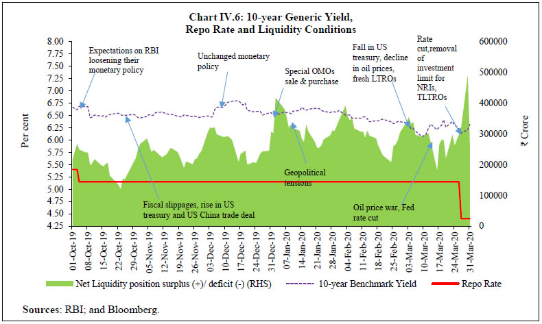 In early-March, yields started with a softening bias of 19 bps and 13 bps in the new and old benchmarks, respectively, due to (i) unscheduled reduction of 150 bps (in two phases) by the Fed in its policy rate; and (ii) fall in crude oil prices due to Saudi Arabia increasing its supply. Yields, however, hardened thereafter due to (i) crude prices firming up in the wake of the US pledging fiscal stimulus to arrest the pandemic; (ii) a sharp depreciation of the INR triggered by COVID-19 driven panic sales by FPIs; and (iii) fears of global recession triggering a shortfall in global dollar liquidity. Yield on the new benchmark, however, fell by 15 bps with announcement of OMO purchases on March 20. The fall in yields was, however, transient as (i) the rupee depreciated to a new record low; and (ii) shrinking G-sec volumes exacerbated the fall in prices. In the backdrop of COVID-19 related stress, the RBI announced several measures on March 27, 2020. In this milieu, while the market frowned over the prospect of larger than expected government borrowings, it welcomed the Reserve Bank’s policy announcement to remove investment limit for non-residents in select dated securities. Overall, the new benchmark fell by 23 bps in March. The yield curve underwent episodic shifts in H2:2019-20, characterised by its level and slope (Chart IV.7a).7 Since the October monetary policy announcement, the average level of the yield softened by 33 bps, while the slope became steeper by 66 bps. Since the February policy announcement (up to March 31, 2020), the average level of the yield softened by 24 bps even as the slope steepened by 58 bps (Chart IV.7b). FPI Investments in G-sec With inflation remaining range bound in October 2019, foreign portfolio investors (FPIs) remained net buyers in the debt market. They turned net sellers, however, till January 2020 on concerns about government finances along with Moody’s downgrading of India's credit rating (to ';negative'; from ';stable”) and fears of sovereign rating downgrade by S&P Global ratings. The lower fiscal deficit projected for 2020-21 in the Union Budget buoyed sentiment and FPIs turned net buyers in February. With heightened turbulence in domestic markets following worldwide financial market meltdown, FPIs again turned net sellers in March (Chart IV.8). Treasury Bills At the shorter end of the primary segment, yields on T-Bills softened during H2:2019-20, tracking the benchmark paper and even traded lower than the reverse repo rate in certain maturities due to surplus liquidity in the banking system (Chart IV.9). The weighted average spread of state development loans (SDLs) cut-off over the corresponding G-sec yield increased to 55 bps in H2 from 52 bps in H1:2019-20 (Chart IV.10). The average inter-state spread on securities of 10-year tenor at 7.2 bps in H2 was higher by 3.2 bps than in H1. Switching of Securities During H2:2019-20, the Reserve Bank conducted seven switch operations amounting to ₹1,24,694 crore for active debt consolidation. This partly contributed to the weighted average maturity (WAM) of outstanding stock of G-secs increasing to 10.54 years as on March 31, 2020 from 10.02 years as on September 30, 2019. As on March 31, 2020, the weighted average coupon (WAC) at 7.69 per cent was lower than 7.77 per cent at end-September 2019. Cash Balance of the Central Government At the beginning of H2:2019-20, the Government started with a negative cash balance and continued to avail ways and means advances/overdraft (WMA/OD) intermittently up to end- March. Cash management bills (CMBs) were issued seven times during H2:2019-20 with maturities between 42-84 days8 for a cumulative amount of ₹2,50,000 crore or 104.2 per cent of the revised estimate of ₹2,40,000 crore of CMBs for 2019-20. IV.1.3 Corporate Bond Market Corporate bond yields eased during H2:2019-20, largely tracking G-sec yields and reflecting surplus systemic liquidity conditions (Chart IV.11a). The AAA 5-year corporate bond yields softened by 42 bps – from 7.44 per cent at end-September 2019 to 7.02 per cent at end-March 2020. Overall, AAA 5-year yields moderated by 108 bps during 2019-20, reflecting the transmission of monetary policy actions to the corporate bond market and the impact of special OMOs and LTRO auctions during December 2019 - March 2020. The risk premia on bonds (5-year AAA corporate bonds over 5-year G-sec) issued by public sector undertakings (PSUs), financial institutions (FIs) and banks reduced by 26 bps while those issued by NBFCs reduced by 14 bps. In contrast, the risk premia on bonds issued by corporates increased by 5 bps. Reflecting the stress in the banking sector from a major private sector bank and declaration of the pandemic, State Bank of India’s and ICICI Bank’s 5-year credit default swap (CDS) spreads increased by 174 bps and 163 bps, respectively, during H2: 2019-20. Resource mobilisation through issuances of corporate bonds in the primary market at ₹3.1 lakh crore during October 2019-February 2020 was higher by 3.0 per cent than ₹3.0 lakh crore during the corresponding period of the previous year (Chart IV.11b). Almost the entire resource mobilisation in the corporate bond market (97.9 per cent) was through the private placement route. In order to provide an alternative source of financing for public sector entities at lower cost and help deepen bond markets by diversifying the investor base with increased retail participation, the Government of India (GoI) launched the Bharat Bond Exchange Traded Fund (ETF) in December 2019 – the first ETF for corporate bonds in India – which mobilised ₹12,395 crore. Investments by FPIs in corporate bonds declined by 14.8 per cent – from ₹2.03 lakh crore at end-September 2019 to ₹1.73 lakh crore at end-March 2020. Consequently, FPIs’ utilisation of the approved limit for investment in corporate bonds declined to 54.5 per cent at end-March 2020 from 66.9 per cent at end-September 2019. The average daily turnover in the corporate bond market increased to ₹8,460 crore during H2:2019-20 (up to March 6, 2020) from ₹7,097 crore during the corresponding period of H2:2018-19. 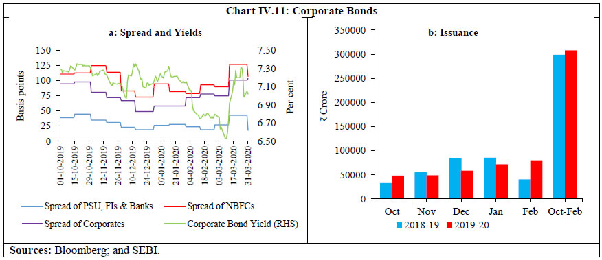 Following the declaration of COVID-19 as a pandemic on March 11, global financial markets were gripped by bearish sentiments. Heightened global turbulence resulted in a significant tightening of financial conditions in India since March 11, 2020 (Chart IV.12). While the spread of secondary market 3-month CP rates of NBFCs over the policy repo rate increased by 108 bps during the period March 11-31, that of AAA corporate bonds of 1-year, 3-year and 5- year maturity increased by 77, 99 and 119 bps, respectively. The spread of the benchmark 10- year G-sec over the policy repo rate also firmed up by 76 bps during the same period. The worsening of financial conditions is attributed to both external and domestic factors. While the upheaval in global markets sparked off panic sales by FPIs in search of safe haven assets, MFs liquidated their positions to create a liquidity buffer in anticipation of redemption pressures from investors. IV.1.4 Equity Market The Indian equity market, which made sizable gains till mid-January 2020, recorded a sharp decline in the remaining part of H2:2019-20 tracking the deterioration in global equity market sentiment due to COVID-19. The BSE Sensex touched the 40,000 level during Q3:2019-20 but it came under intense pressure during Q4: 2019-20. Overall, the Sensex declined by 23.8 per cent during H2:2019-20 (Chart IV.13a). The BSE Sensex reclaimed the 40,000 level on October 30, 2019 taking positive cues from global markets amidst fresh optimism over the US-China trade negotiations and agreement on Brexit deal between the UK and the European Union (EU). The uptrend continued in November and December on the back of growth boosting measures by the Government of India (GoI), support to the Insolvency and Bankruptcy Code amendment and approval for a partial credit guarantee scheme for public sector banks to purchase pooled assets from NBFCs. Furthermore, positive global signals emanating from the US Fed’s dovish outlook, the US-China phase one trade deal and Brexit favouring UK election outcome also brightened market sentiment. 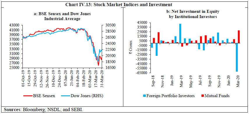 The buoyancy in the equity market continued till mid-January 2020 against the backdrop of a fall in global crude prices, recovery in industrial output in November, higher GST collection and expansion in manufacturing Purchasing Managers’ Index (PMI) in December which pushed the Sensex to a record close of 41953 on January 14, 2020. Markets wilted, however, following the escalation of geo-political tensions between the US and Iran, a subdued domestic GDP growth outlook along with downward revision of India’s growth forecast for 2019-20 by the International Monetary Fund (IMF). The decline got accentuated on February 1, 2020 with the Sensex plunging by 988 points (2.4 per cent) as proposals in the Union Budget 2020-21 fell short of market expectations. A V-shaped recovery, however, was witnessed on the back of a sharp fall in crude oil prices, release of robust PMI data for January 2020 and announcement of credit and liquidity enhancing measures on February 6, 2020. Subsequently, Indian equity markets retracted in line with global markets reacting to COVID-19. Growing risk aversion across the world triggered heavy sell-offs in equity markets, including in India, during March 2020. The BSE Sensex fell by 2919 points (8.2 per cent) on March 12, 2020. Market sentiment worsened the following day as market fell over 10 per cent during early hours of trading, attracting circuit breakers and suspension of trading for 45 minutes. This was followed by a statement from SEBI indicating that the fall in the Indian stock indices had been significantly lower than in many other countries and assuring market participants of suitable and appropriate actions, if required. Market rebounded, ending the day with a net gain of 1325 points (4.0 per cent), the largest ever recovery in a single day. Subsequently, however, bearish momentum returned due to (i) sharp moderation in global crude prices; (ii) reports of a spike in COVID-19 cases in India; (iii) strain on the banking sector caused by the distress of a private sector bank; and (iv) growing worries about global recession. Consequently, the Indian equity market breached the lower circuit for the second time during March 2020 with the BSE Sensex recording its biggest fall of 3,935 points (13.2 per cent) on March 23, 2020. Markets recovered thereafter amid expectations of fiscal measures by the government after the announcement of extension of regulatory deadlines and relaxation of norms for corporates and taxpayers. Subsequently, expectations of more fiscal stimulus buoyed market sentiment. Notwithstanding the announcement of comprehensive liquidity measures by the Reserve Bank including sizeable reduction in policy rates, the BSE Sensex fell marginally on March 27. Overall, the BSE Sensex registered a sharp decline of 23.0 per cent during March 2020. During H2, while MFs were net buyers to the tune of ₹ 38,989 crore (up to March 30), FPIs were net sellers at ₹5,599 crore in the Indian equity market (Chart IV.13b). FPIs, in particular, sold heavily with net sales amounting to ₹62,433 crore in March 2020. In the primary segment of the equity market, resource mobilisation through public issues of equity (initial public offers and right issues) remained muted at ₹6,176 crore during October 2019-February 2020 (although higher than ₹3,429 crore in the corresponding period of the previous year). IV.1.5 Foreign Exchange Market The INR remained volatile during H2:2019-20 due to multiple factors referred to in preceding sections and the high volatility in equity markets. Portfolio investment was severely impacted. Consequently, EME currencies, including the INR, weakened sharply in March, with the latter depreciating to a low of ₹76.15 on March 24, 2020. While the INR depreciated by 6.2 per cent vis-à-vis the US dollar during H2:2019-20 (end-March 2020 over end-September 2019), the decline was modest in comparison with many EME peers such as the Thai baht, the Argentine peso, the Indonesian rupiah, the Turkish lira, the South African rand, the Mexican peso, the Russian rubble, and the Brazilian real (Chart IV.14a). In terms of the 36-currency nominal effective exchange rate (NEER), the INR depreciated by 2.9 per cent (as at end-March 2020 over average of September 2019). The INR also depreciated by 1.3 per cent in terms of the 36-currency real effective exchange rate (REER) during the same period (Table IV.2). Table IV.2: Nominal and Real Effective Exchange Rates – Trade-based Weights
(Base: 2004-05 = 100) | | Item | Index: end-March 2020 (P) | Appreciation (+) / Depreciation (-) (Per cent) | | end-March 2020 over September (average) 2019 | | 36-currency REER | 114.6 | -1.3 | | 36-currency NEER | 71.1 | -2.9 | | 6-currency REER | 120.3 | -4.5 | | 6-currency NEER | 60.3 | -5.5 | | ₹/ US$ | 75.4 | -5.4 | P: Provisional.
Sources: RBI; and FBIL. | Between September 2019 and February 2020, the appreciation of the INR in terms of the REER was modest as compared with those of the Russian ruble, the Indonesian rupiah, the Philippine peso, the Chinese yuan, the Mexican peso, and the Argentine peso (Chart IV.14b). IV.1.6 Credit Market Credit offtake during 2019-20 (up to March 13, 2020) was muted with non-food credit growth at 6.1 per cent being less than half the growth of 14.4 per cent in the corresponding period of the previous year. Both low momentum and unfavourable base effects were at work (Chart IV.15). The seasonal decline in Q3 credit growth in 2019-20 was more pronounced than a year ago, while the offtake during Q4:2019-20 (up to March 13) has been subdued as compared with the corresponding quarters of previous two years. 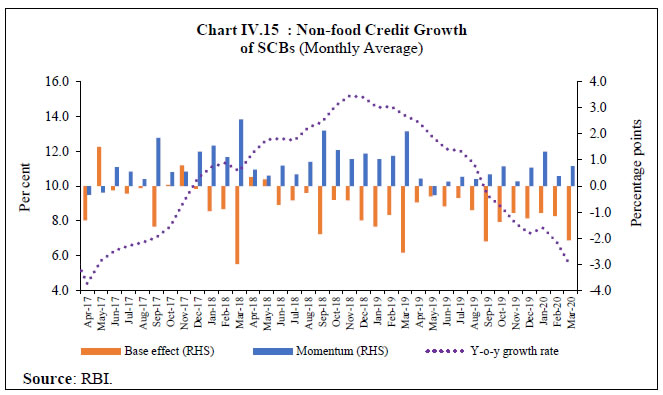 The slowdown in credit growth was spread across all bank groups, especially private sector banks. Credit growth of public sector and foreign banks remained modest, even as there has been some uptick in credit by public sector banks in the recent period (Chart IV.16). Of the incremental credit extended by scheduled commercial banks (SCBs) during the year (March 15, 2019 to March 13, 2020), 62.6 per cent was provided by private sector banks, 36.6 per cent by public sector banks and 0.8 per cent by foreign banks. 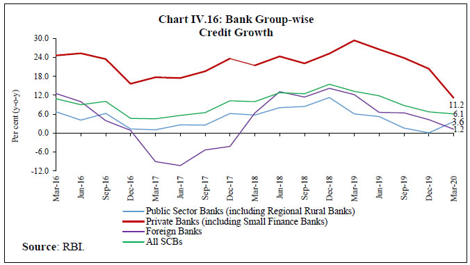 While growth (y-o-y) of personal loans accelerated marginally to 17.0 per cent in February 2020 from 16.7 per cent in February 2019, credit growth to both agriculture and industry moderated over the last five months. Although credit growth to the services sector showed an uptick in January 2020, it again weakened in February 2020 (Chart IV.17a). Credit offtake in personal loans segment accounted for the largest share (Chart IV.17b). Within the personal loan segment, credit offtake has been mainly concentrated in housing and credit card outstandings. Within industry, credit growth to beverage and tobacco accelerated, but credit flows to chemical and chemical products, cement and cement products, construction and infrastructure decelerated. Credit to basic metal and metal products, textiles, food processing and all engineering contracted in February 2020. 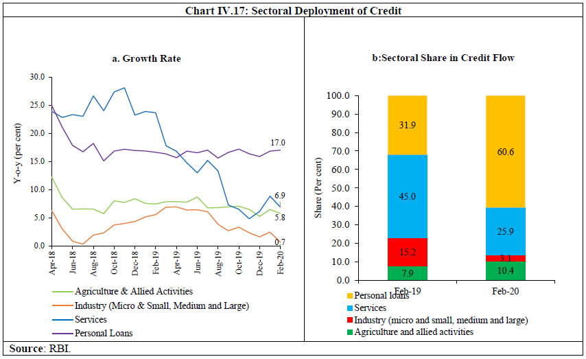 Even as the overall non-performing assets (NPA) ratio of SCBs remained unchanged in December 2019 from end-March 2019 (Chart IV.18a), the NPA ratio in respect of industry dipped (Chart IV.18b). Banks’ investments in CPs, bonds, debentures and shares of public and private corporates – reflected in non-SLR investment – were lower during H2:2019-20 (up to March 13) than a year ago mainly due to lower investment in bonds/shares and debentures (Chart IV.19a). As a result, adjusted non-food credit growth was lower in Q4:2019-20 (up to March 13) than in Q3 (Chart IV.19b). With credit offtake remaining muted and non-SLR investments declining, banks augmented their SLR portfolios. Banks held excess SLR of 8.4 per cent of net demand and time liabilities (NDTL) on Feb 28, 2020 as compared with 6.3 per cent of NDTL at end-March 2019 (Chart IV.20). IV.2 Monetary Policy Transmission Since the October 2019 Monetary Policy Report, monetary policy transmission to banks’ term deposit and lending interest rates has improved (Table IV.3). The pass-through of the policy rate cut to the weighted average domestic term deposit rate (WADTDR) on outstanding rupee deposits improved to 39 bps during October 2019-February 2020 from a mere 7 bps during the previous eight months (February-September 2019), resulting in an overall reduction of 46 bps. The weighted average lending rate (WALR) on outstanding rupee loans has also declined by 18 bps since October 2019 in contrast to a rise of 2 bps during February-September 2019. The WALR on fresh rupee loans declined by 71 bps (February 2019-February 2020). Of this, a decline of 31 bps occurred during October 2019-February 2020. | Table IV.3: Transmission to Deposit and Lending Rates | | (Basis points) | | Period | Repo Rate | Term Deposit Rates | Lending Rates | | Median Term Deposit Rate | WADTDR | 1-year Median MCLR | WALR - Outstanding Rupee Loans | WALR - Fresh Rupee Loans | | February- September 2019 | -110 | -9 | -7 | -30 | 2 | -40 | | October 2019- March 2020* | -100 | -29 | -39 | -30 | -18 | -31 | | February 2019- March 2020* | -210 | -48 | -46 | -60 | -16 | -71 | *: Latest data on WALR and WADTDR pertain to February 2020.
WADTDR: Weighted Average Domestic Term Deposit Rate. WALR: Weighted Average Lending Rate.
MCLR: Marginal Cost of Funds-based Lending Rate.
Source: RBI. | The improvement in transmission during H2:2019-20 to banks’ deposit and lending interest rates reflected the lagged impact of the previous rate cuts (110 bps during February–September 2019) as also the introduction of the external benchmark system from October 1, 2019 for the pricing of new floating rate loans to select sectors, viz., retail loans and loans to micro and small enterprises (MSEs). 9 During February 2019 - February 2020, the WALR on fresh rupee loans declined across bank groups, with the largest decline observed in the case of foreign banks, followed by public sector banks (Chart IV.21). The median spread10 [WALR on fresh rupee loans over 1-year median marginal cost of funds-based lending rate (MCLR)] charged by private sector banks was higher than that of public sector banks, reflecting, inter alia, differences in the lending portfolio (Chart IV.22). Sector-specific WALRs in respect of sectors such as micro, small and medium enterprises (MSMEs), credit card and other personal loans were higher than the overall WALR for both public and private sector banks. The share of loans to each of these sectors in total loans sanctioned by private sector banks was higher than that of public sector banks. 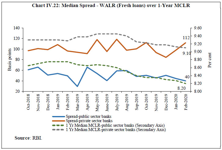 The share of public sector banks in fresh rupee loans sanctioned by scheduled commercial banks was comparable to that of private sector banks during April-August 2019, even though public sector banks account for a significantly larger share in outstanding credit. In comparison with private sector banks, non-performing assets of public sector banks have been higher and the capital to risk weighted assets ratio (CRAR) lower. Despite this, the share of public sector banks in total fresh rupee loans sanctioned by scheduled commercial banks increased to 52.8 per cent from a low of 39.7 per cent in August 2019 (Chart IV.23). 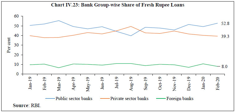 Spreads, i.e., WALR on outstanding rupee loans over 1-year MCLR charged by scheduled commercial banks, were lowest in respect of housing loans, reflecting lower probability of default and availability of collateral, as also competition from NBFCs (Chart IV.24). Personal loans – other than housing, vehicles and education – are mostly unsecured and involve higher credit risk; hence, the spread charged was the highest for ‘other personal loans’. The spreads between lending rates in the credit market and corporate bond yields have risen sharply since January 2019, implying faster transmission of policy rate cuts to the corporate bond market as against relatively muted transmission to the credit market (Chart IV.25). Following the introduction of the external benchmark system in the banking sector on October 1, 2019, 36 banks – out of 62 banks from whom information was collected – adopted the policy repo rate as the external benchmark for floating rate loans to the retail and MSE sectors (Table IV.4). Six banks have linked their loans to various other benchmarks published by Financial Benchmarks India Private Ltd (FBIL) such as CD rate, overnight index swap (OIS) rate, Mumbai Interbank Outright Rate (MIBOR) and 3-month T-Bill rate. Eleven banks have linked different sectors to different benchmarks. | Table IV.4: External Benchmarks of Commercial Banks: February 2020 | | Bank Group | Policy Repo Rate | CD Rate | OIS Rate | MIBOR | 3-Month T-Bill Rate | Sector-specific Benchmark | | Public Sector Banks (15) | 14 | - | - | - | - | 1 | | Private Banks (20) | 15 | 1 | | - | - | 4 | | Foreign Banks (27) @ | 7 | - | 1 | 1 | 3 | 6 | | Commercial banks (62) @ | 36 | 1 | 1 | 1 | 3 | 11 | @ 9 banks do not have any exposure to retail loans and MSE loans segments.
Note: Figures in parentheses refer to the number of banks.
Source: RBI. | The median spread in respect of fresh rupee loans linked to the policy repo rate (i.e., median WALR over the repo rate) was the highest for ‘other personal loans’ (Table IV.5). Among the bank-groups, the median spread charged by public sector banks for different categories of loans was lower than that charged by private sector banks. | Table IV.5: Loans Linked to the Policy Repo Rate - Median Spread (February 2020) | | (Percentage points) | | Bank Group | Personal Loan | Micro and Small Enterprises | | Housing | Vehicle | Education | Other Personal Loans | | Public Sector Banks (15) | 3.3 | 4.6 | 4.2 | 6.7 | 5.8 | | Private Sector Banks (20) | 5.3 | 6.2 | 6.8 | 7.1 | 6.4 | | Domestic Banks (35) | 4.0 | 4.9 | 4.6 | 6.8 | 6.1 | | Source: RBI. | There are early indications of an improvement in transmission to fresh rupee loans sanctioned in respect of sectors where new floating rate loans have been linked to the external benchmark. During October 2019 - February 2020, the WALRs of domestic (public and private sector) banks declined in respect of fresh rupee loans sanctioned for housing loans by 34 bps, vehicle loans by 73 bps, education loans by 21 bps and micro, small and medium enterprises (MSMEs) by 6 bps (Chart IV.26). 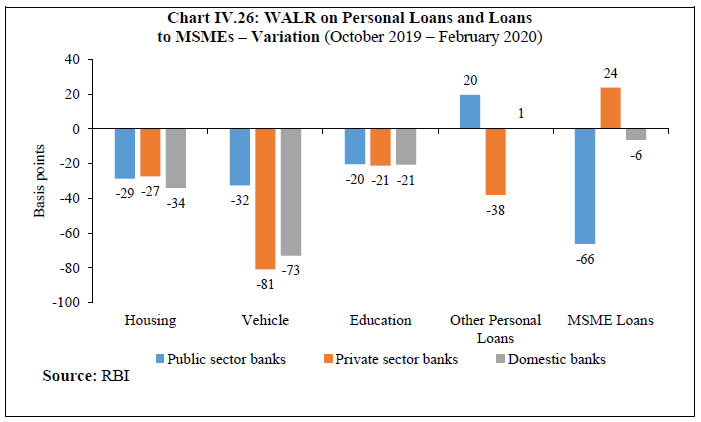 Administered interest rates on small saving schemes set by the Government of India have implications for monetary transmission. These administered interest rates are linked to market yields on G-secs with a lag and are fixed on a quarterly basis at a spread ranging from 0-100 bps over and above G-sec yields of comparable maturities. On March 31, 2020, the Government of India sharply reduced rates of interest on all small saving schemes (except saving deposit) in the range of 70-140 bps for Q1:2020-21. Following the revision, interest rates on small saving schemes for Q1:2020-21 are broadly aligned with the prescribed formula based administered interest rates on small savings (Table IV.6). This augurs well for monetary transmission, going forward. | Table IV.6: Interest Rates on Small Saving Instruments - Q1:2020-21 | | Small Savings Scheme | Maturity (years) | Spread (Percentage point) $ | Average G-sec yield (%) of Corresponding Maturity (December 2019 to February 2020) | Formula based Rate of Interest (%) (Applicable for Q1: 2020-21) | Government Announced Rate of Interest (%) (Q1:2020-21) | Difference between Government Announced Rate and the Formula- based Rate (basis points) | | (1) | (2) | (3) | (4) | (5) = (3) + (4) | (6) | (7) = (6)-(5) | | Savings Deposit | - | - | - | - | 4.00 | - | | Public Provident Fund | 15 | 0.25 | 6.88 | 7.13 | 7.10 | -3 | | Term Deposits | | | | | | | | 1 Year | 1 | 0 | 5.15 | 5.15 | 5.50 | 35 | | 2 Year | 2 | 0 | 5.47 | 5.47 | 5.50 | 3 | | 3 Year | 3 | 0 | 5.78 | 5.78 | 5.50 | -28 | | 5 Year | 5 | 0.25 | 6.41 | 6.66 | 6.70 | 4 | | Post Office Recurring Deposit Account | 5 | 0 | 5.78 | 5.78 | 5.80 | 2 | | Post Office Monthly Income Scheme | 5 | 0.25 | 6.38 | 6.63 | 6.60 | -3 | | Kisan Vikas Patra | 124 Months | 0 | 6.88 | 6.88 | 6.90 | 2 | | NSC VIII issue | 5 | 0.25 | 6.57 | 6.82 | 6.80 | -2 | | Senior Citizens Saving Scheme | 5 | 1.00 | 6.41 | 7.41 | 7.40 | -1 | | Sukanya Samriddhi Account Scheme | 21 | 0.75 | 6.88 | 7.63 | 7.60 | -3 | $: Spreads for fixing small saving rates as per Government of India Press Release of February 16, 2016.
Note: Compounding frequency varies across instruments.
Sources: Government of India; and RBI staff estimates. | IV.3. Liquidity Management and the Operating Procedure of Monetary Policy The RBI Act, 1934 amended in 2016 requires the RBI to place the operating procedure relating to the implementation of monetary policy and changes thereto from time to time, if any, in the public domain. During H2:2019-20, liquidity management operations by the RBI were conducted in line with the revised liquidity management framework announced on February 6, 2020 and guided by the need to ease liquidity constraints in the banking system and financial markets on account of COVID-19 related stress (Box IV.2). During H1 and a major part of H2:2019-20, systemic liquidity increased mainly on account of (i) the Reserve Bank’s forex operations; and (ii) higher spending by the government, including recourse to WMA and OD. In order to mop up the increasing surplus liquidity, the Reserve Bank conducted variable rate reverse repo auctions of various tenors (ranging from overnight to 63 days including the main 14-day term reverse repo auction conducted on reporting Fridays since February 14, 2020) amounting to ₹1,96,02,726 crore in H2. Moreover, five LTROs were conducted during February and March with a view to ensuring monetary transmission. Furthermore, one targeted long term repo operation (TLTRO) was conducted in March to address the COVID-19 induced pressure on financial conditions. Box IV.2: Revised Liquidity Management Framework As announced in the Statement on Developmental and Regulatory Policies of June 6, 2019, an Internal Working Group was set up to review the liquidity management framework with a view to simplifying it and suggesting measures to clearly communicate the objectives and the toolkit for liquidity management. The Group’s report was placed on the Reserve Bank’s website on September 26, 2019 for comments from stakeholders and members of the public (RBI, 2019). Based on the feedback received, it was decided to fine-tune the erstwhile liquidity management framework. The key elements of the revised framework are set out below: -
Liquidity management remains the operating procedure of monetary policy; the weighted average call rate (WACR) continues to be its operating target. -
The liquidity management corridor is retained, with the marginal standing facility (MSF) rate as its upper bound (ceiling) and the fixed rate reverse repo rate as the lower bound (floor), with the policy repo rate in the middle of the corridor. -
The width of the corridor is retained at 50 basis points – the reverse repo rate being 25 basis points below the repo rate and the MSF rate 25 basis points above the repo rate.11 -
The daily fixed rate repo and four 14-day term repos conducted every fortnight earlier, have been withdrawn. The Reserve Bank, however, would ensure adequate provision/absorption of liquidity as warranted by underlying and evolving market conditions – unrestricted by quantitative ceilings – at or around the policy rate. -
Instruments of liquidity management continue to include fixed and variable rate repo/reverse repo auctions, outright open market operations (OMOs), forex swaps and other instruments as may be deployed from time to time to ensure that the system has adequate liquidity at all times. -
A 14-day term repo/reverse repo operation at a variable rate and conducted to coincide with the cash reserve ratio (CRR) maintenance cycle is the main liquidity management tool for managing frictional liquidity requirements. -
The main liquidity operation would be supported by fine-tuning operations, overnight and/or longer tenor, to tide over any unanticipated liquidity changes during the reserve maintenance period. -
In addition, the RBI will conduct, if needed, longer-term variable rate repo/reverse repo operations of more than 14 days. -
The current requirement of maintaining a minimum of 90 per cent of the prescribed CRR on a daily basis will continue.12 -
Standalone Primary Dealers (SPDs) were allowed to participate directly in all overnight liquidity management operations. -
The margin requirements under the Liquidity Adjustment Facility (LAF) would be reviewed on a periodic basis; the margin requirement for reverse repo transactions, however, would continue to be ‘Nil’. -
In order to improve communication on the RBI’s liquidity management framework and procedures, the following measures were introduced: (a) the Press Release detailing Money Market Operations (MMO) was modified suitably to show both the daily flow impact as well as the stock impact of the RBI’s liquidity operations; (b) the Reserve Bank started publishing a quantitative assessment of durable liquidity conditions of the banking system on a fortnightly basis with a lag of one fortnight; and (c) periodic consultations will be conducted with market participants and other stakeholders. Reference: Reserve Bank of India (2019), “Report of the Internal Working Group to Review the Liquidity Management Framework”, September 26. | In view of the COVID-19 pandemic and its adverse impact on global and domestic financial markets, the MPC advanced its meeting in an unprecedented move, after a careful evaluation of the current and evolving macroeconomic and financial conditions, and the outlook. The MPC voted for an unprecedented 75 bps reduction in the policy repo rate and for continuing with the accommodative stance as long as necessary to revive growth and mitigate the impact of COVID-19 on the economy, while ensuring that inflation remains within the target. Alongside, several measures were also announced on March 27, 2020 to address the stress in financial conditions and ease COVID-19 related liquidity constraints (Box IV.3). Box IV.3: Liquidity Measures to Combat Adverse Impact of COVID-19 (I) Targeted Long-Term Repo Operations (TLTROs) Reserve Bank to conduct auctions of targeted long-term repos of up to three years tenor of appropriate sizes for a total amount of up to ₹1,00,000 crore at a floating rate linked to the policy repo rate. Liquidity availed by banks under TLTROs should be deployed in investment grade corporate bonds, commercial paper, and non-convertible debentures over and above the outstanding level of their investments in these bonds as on March 27, 2020. (II) Cash Reserve Ratio (CRR) (i) CRR requirement of banks was reduced by 100 bps from 4.0 per cent of NDTL to 3.0 per cent effective fortnight beginning March 28, 2020, which would augment primary liquidity in the banking system by about ₹1,37,000 crore. This dispensation will be available for a period of one year ending March 26, 2021. (ii) The minimum daily CRR balance requirement was reduced from 90 per cent to 80 per cent effective from the first day of the fortnight beginning March 28, 2020. This dispensation will be available up to June 26, 2020. (III) Marginal Standing Facility (MSF) In view of the exceptionally high volatility in domestic financial markets and to provide comfort to the banking system, banks’ limit for borrowing overnight under the MSF by dipping into their Statutory Liquidity Ratio (SLR) were raised to 3 per cent of NDTL from 2 per cent. This measure will allow the banking system to avail an additional ₹1,37,000 crore of liquidity under the liquidity adjustment facility (LAF) window at the reduced MSF rate of 4.65 per cent and will be applicable up to June 30, 2020. (IV) Reduction in Policy Rate and Widening of the Policy Corridor (i) The policy repo rate under the LAF was reduced by 75 basis points to 4.40 per cent from 5.15 per cent with immediate effect. Accordingly, the MSF rate and the Bank Rate were reduced to 4.65 per cent from 5.40 per cent. (ii) In view of persistent excess liquidity, the existing LAF corridor was widened asymmetrically to 65 bps from 50 bps. Accordingly, the reverse repo rate was reduced by 90 bps from 4.90 per cent to 4.00 per cent. The purpose of this measure was to make it relatively unattractive for banks to passively deposit funds with the RBI; instead, these funds should be deployed for on-lending to productive sectors of the economy. (iii) Thus, the reverse repo rate is now 40 bps lower than the policy repo rate while the MSF rate continues to be 25 bps above the policy repo rate. Reference: Reserve Bank of India (2020), “Statement on Developmental and Regulatory Policies”, March 27. | Drivers and Management of Liquidity The leakage of currency from the system during H2:2019-20 was more than offset by Reserve Bank’s forex operations and drawdown of government cash balances, thereby augmenting liquidity in the banking system (Chart IV.27). The surplus liquidity was absorbed through reverse repo operations under the LAF. The increase in currency in circulation (CiC) of ₹2.61 lakh crore in H2 was more than five-fold than that of ₹49,378 crore in H1:2019-20 and higher than ₹2.11 lakh crore in H2:2018-19. As a result, growth in CiC at 11.9 per cent during H2:2019-20 was higher than 11.0 per cent during the corresponding period of 2018-19. 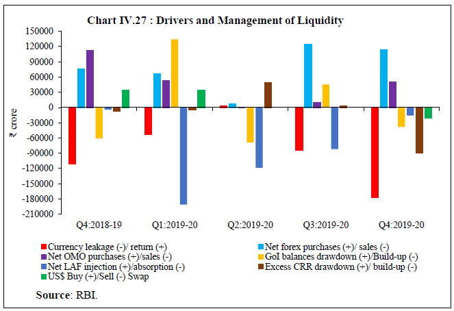 Surplus liquidity conditions persisted in Q3:2019-20 as daily net liquidity absorption under the LAF progressively increased from ₹1.99 lakh crore in October to ₹2.41 lakh crore in November and further to ₹2.61 lakh crore in December 2019. Expecting the continuance of surplus liquidity, the Reserve Bank conducted four longer term reverse repos auctions in November – two of 21-days and one each of 42-days and 35-days tenor – thereby absorbing ₹78,934 crore. During Q3, the Reserve Bank’s forex operations (₹1.25 lakh crore) and drawdown of GoI cash balances (₹45,184 crore) augmented systemic liquidity. The Reserve Bank also conducted four special OMOs during December and January (December 23 and 30, 2019 and January 6 and 23, 2020), which augmented net banking system liquidity by ₹11,724 crore.13 In Q4, average daily surplus liquidity further increased to ₹3.18 lakh crore in January as the Government continued to avail WMA/OD for the entire month, but moderated to ₹2.98 lakh crore in February as GoI’s cash balance turned positive in the second half of the month, due to issuance of CMBs as discussed earlier (see IV.1.2 for details). In March, average daily net absorption under the LAF amounted to ₹3.02 lakh crore. Taking into consideration the increased demand for US dollars amidst flight to safety triggered by extremely volatile global financial markets, the Reserve Bank conducted two 6-month US Dollar/INR sell/buy swap auction on March 16 and March 23, 2020, which cumulatively provided dollar liquidity of USD 2.71 billion (Chart IV.28). Furthermore, in view of hardening yields and widening spreads in certain market segments symptomatic of stressed financial conditions (see Chart IV.12), three open market purchase operations were conducted on March 20, 24 and 26, 2020, thereby injecting ₹40,000 crore cumulatively. 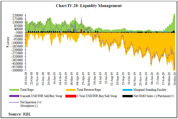 With a view to reinforcing monetary transmission and augmenting credit flows to productive sectors, the Reserve Bank conducted five long term repo operations (LTRO) at fixed repo rate (one of one-year and four of three-year tenors) between February 17 and March 18, 2020, which infused durable liquidity amounting to ₹1.25 lakh crore into the system with additional ₹75,000 crore in the pipeline. The LTROs provided banks with durable liquidity at reasonable cost (fixed repo rate) relative to prevailing market rates. Moreover, a TLTRO auction of 3-year maturity held on March 27, 2020 also augmented durable liquidity by ₹25,009 crore.14 Thus, total durable liquidity (including forex purchases, OMOs, LTROs and TLTRO) amounting to ₹4,49,326 crore was injected in H2:2019-20 as compared with ₹1,26,514 crore in H1 (Chart IV.29). 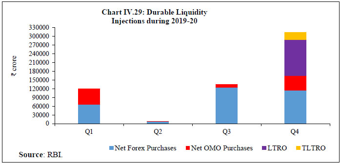 Summing up, currency expansion, Reserve Bank’s forex operations and government spending were the key liquidity drivers in the banking system during H2:2019-20 (Chart IV.30). 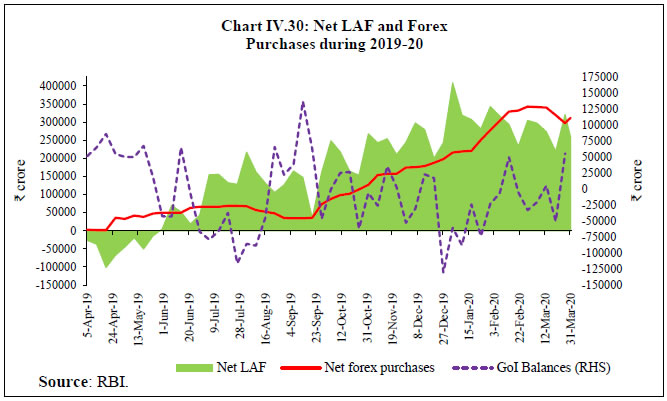 Given surplus liquidity conditions, fine-tuning operations through variable rate reverse repo auctions with maturity ranging from overnight to 3 days were extensively used for absorbing liquidity till February 14, 2020. As a pre-emptive measure to tide over any frictional liquidity requirements caused by dislocations due to COVID-19, two fine-tuning variable rate repo auctions of 16-day maturity were conducted on March 23 and March 24, 2020 injecting ₹77,745 crore cumulatively (Table IV.7). To address any additional demand for liquidity and provide flexibility to the banking system in its liquidity management towards the year-end, one fine-tuning variable rate repo auction of 12-days maturity was conducted on March 26 injecting ₹11,772 crore.15 As a special case, SPDs were allowed to participate in these auctions along with other eligible participants. | Table IV.7: Fine-tuning Operations Through Variable Rate Auctions in H2:2019-20 | | Repo | Reverse Repo | | Maturity in Days | 12, 16 | 1-3 | 4 | 21 | 28-29 | 31 | 35 | 42 | 63 | | Number of Operations | 3 | 90 | 2 | 2 | 3 | 1 | 1 | 2 | 3 | | Total Volume (₹ crore) | 89,517 | 1,85,67,948 | 3,21,328 | 28,923 | 47,165 | 12,790 | 25,004 | 30,507 | 65,033 | | Average Volume (₹ crore) | 29,839 | 2,06,311 | 1,60,664 | 14,462 | 15,722 | 12,790 | 25,004 | 15,254 | 21,678 | | Source: RBI. | IV.4 Conclusion Domestic financial markets remain vulnerable to global developments, deepening of the growth slowdown in India and rising concerns about COVID-19. Despite the weak domestic growth outlook, Indian equity markets scaled new highs, before turning highly volatile in early- March in tandem with global equity markets. The outlook is characterised by heightened uncertainty with capital outflows continuing and exerting pressures on the INR. This outlook is uncertain and is increasingly getting reflected in bond market yields. Credit growth is likely to remain modest, reflecting weak demand and risk aversion. Going forward, liquidity conditions would be managed under the revised liquidity management framework, consistent with the accommodative stance of monetary policy as long as necessary to revive growth and mitigate the impact of COVID-19, while ensuring that inflation remains within the target. Better transmission of monetary policy impulses to the credit market would remain a priority. __________________________________________________________________
V. External Environment Economic activity remained subdued across major advanced economies (AEs) and emerging market economies (EMEs). Though some transitory signs of stabilisation were evident in early 2020, the outbreak of COVID-19 and its rapid spread over a large number of countries has clouded the near-term outlook. Monetary policy has remained highly accommodative as most central banks across the world resorted to massive easing through both conventional and unconventional measures. Global financial markets, which remained buoyant on risk-on sentiments in Q4:2019, slumped on sell-off pressures triggered by intensifying COVID-19 disruptions. Global economic activity remained subdued during the major part of H2:2019. In January 2020, the IMF estimated global GDP growth at 2.9 per cent for 2019, the lowest since the global financial crisis (GFC). Early into 2020, signs of stabilisation seemed to appear in the form of de-escalating trade tensions between the US and China and receding possibility of a hard Brexit. A pneumonia of unknown cause detected in Wuhan, China first reported to the World Health Organization (WHO) on December 31, 2019 delivered a cataclysmic shock to these green shoots and changed the world. The WHO declared a Public Health Emergency of International Concern on January 30, 2020 and christened the novel coronavirus as COVID-19 on February 11, 2020. On March 11, 2020, the WHO declared it a pandemic – “the first pandemic caused by a corona virus”1. At the time of going to press, more than 12 lakh people were infected around the world with more than 67,000 deaths2. In the G-20 Ministerial Call on the Coronavirus Emergency on March 23, 2020 the Managing Director, IMF formally informed that the global economy had entered into recession in 2020. Amongst the early incoming data, GDP of Singapore shrank by 10.6 per cent in Q1:2020. In the US, jobless claims surged to a peak as the number of people filling for unemployment insurance claims jumped to 6.6 million in the week ended March 28, 2020, the highest since the series began in 1967. Crude oil prices plummeted in March due to price war between Saudi Arabia and Russia over disagreement on production cuts. Prices of other global commodities ebbed on fears of weakening global demand. Prices of precious metals initially rallied on safe haven demand as investors resorted to flight to safety, but they declined in the second week of March as investors preferred to hold cash. Central banks across major advanced economies (AEs) and emerging market economies (EMEs) switched to highly accommodative mode, with most of them resorting to rate cuts in unscheduled meetings. Central banks also announced several liquidity measures and regulatory relaxations in the face of tightening financial conditions. Fiscal authorities across the world have launched stimuli in the range of 0.8-16.0 per cent of their GDP. Besides direct support, measures also include tax deferment and credit guarantee. V.1 Global Economic Conditions In the US, GDP grew by 2.1 per cent in Q4:2019 – the same pace as in the previous quarter. Overall GDP growth for 2019 decelerated to its slowest pace in three years amidst continuing weakness in business investment and exports (Table V.1). In Q1:2020, industrial production growth stalled in March after contracting for the fifth consecutive month in January and the manufacturing purchasing managers’ index (PMI) of the Institute for Supply Management (ISM) contracted in March after improving marginally in January-February. Retail sales have also softened since January. Although labour market remained strong in February as reflected in better than expected US jobs report, number of people filling jobless claims in the US for the week ended March 28 rose to a record level of 6.6 million – the highest since the series began in 1967. Economic activity in the Euro area decelerated markedly in Q4:2019 as a pronounced downturn in industrial activity and subdued consumer demand weighed on overall economic performance. GDP growth contracted in France and Italy in Q4:2019 on waning consumer confidence, and stagnated in Germany on muted private and government spending. In Q1:2020, the rapid spread of COVID-19 infections in Italy, Spain and other European countries is likely to impact manufacturing and services sectors. The ECB has projected GDP growth to decline to 0.8 per cent for 2020 under its baseline scenario assumption that the impact of virus would get contained in next few months and growth would normalise in H2:2020. | Table V.1: Real GDP Growth (q-o-q, annualised) | | (Per cent) | | Country | Q4-2018 | Q1-2019 | Q2-2019 | Q3-2019 | Q4-2019 | 2020 (P) | 2021 (P) | | Advanced Economies | | Canada | 1.0 | 1.0 | 3.4 | 1.1 | 0.3 | 1.8 | 1.8 | | Euro area | 1.2 | 1.6 | 0.8 | 1.2 | 0.4 | 1.3 | 1.4 | | Japan | 2.4 | 2.2 | 2.3 | 0.1 | -7.1 | 0.7 | 0.5 | | South Korea | 3.6 | -1.6 | 4.0 | 1.6 | 5.2 | 2.2 | 2.7 | | UK | 0.8 | 2.4 | -0.4 | 2.0 | 0.0 | 1.4 | 1.5 | | US | 1.1 | 3.1 | 2.0 | 2.1 | 2.1 | 2.0 | 1.7 | | Emerging Market Economies | | Brazil | 0.0 | 0.0 | 2.0 | 2.4 | 2.0 | 2.2 | 2.3 | | China* | 6.5 | 6.4 | 6.2 | 6.0 | 6.0 | 6.0 | 5.8 | | Indonesia* | 5.2 | 5.1 | 5.1 | 5.0 | 5.0 | 5.0 | 5.1 | | Russia* | 2.7 | 0.5 | 0.9 | 1.7 | 2.1 | 1.9 | 2.0 | | South Africa | 1.4 | -3.2 | 3.3 | -0.8 | -1.4 | 0.8 | 1.0 | | Thailand | 5.2 | 3.2 | 1.4 | 0.6 | 1.0 | 3.0 | 3.5 | | Memo: | 2019 (E) | 2020 (P) | 2021 (P) | | World Output | 2.9 | 3.3 | 3.4 | | World Trade Volume | 1.0 | 2.9 | 3.7 | E: Estimate P: Projection *: y-o-y growth
Sources: Bloomberg; and International Monetary Fund. | The Japanese economy contracted sharply in Q4 as private consumption slumped in the wake of October’s sales tax hike. The slowdown in factory activity due to a string of typhoons and sluggish external demand added further pressure on domestic activity. In Q1:2020, the increased number of infections, including across the East Asian regions, threaten to disrupt economic activity severely. In the UK, GDP growth stagnated in Q4, after rebounding in Q3. Positive contributions from the services and construction sectors were offset by a decline in manufacturing output. Political uncertainty due to the Brexit deadline in October and general election in December appeared to have slowed activity in the final quarter. In Q1:2020, industrial production contracted and retail sales remained subdued. Risks emanating from COVID-19 may undermine the outlook for Q1. Sluggish growth across major EMEs in Q4:2019 was overwhelmed by the outbreak of COVID-19; suddenly, the downside risks to growth became acute (Box V.1). Box V.1: Impact of COVID-19 on Global Growth In the initial weeks of February, most forecasts of global output loss due to COVID-19 were in terms of the outbreak being confined to China and being brought under control by March/June. It was, however, acknowledged that even in the limited scenario, the economic impact would be significant as China is a much larger player – both in terms of economic size and its role in global value chains – now than in 2003, the period of the SARS epidemic (Chart V.1.1). Owing to extended lunar new year holidays as also government-imposed factory shutdowns and travel restrictions in a number of regions, China’s manufacturing/services activity declined sharply in February. In the latter part of February, a rapid surge of infections and fatalities around the world began to surface, even as the spread of the virus in China began to plateau. Lockdowns were/have been imposed in most countries. Travel bans have created distress for airlines, tourism and hospitality industries. In the commodity and financial markets, crude oil prices have been on a downward spiral; with West Texas intermediate (WTI) crude prices crashing below US$ 20 per barrel on March 30, 2020. Equity markets have suffered major losses, while gold, fixed income assets – mainly government debt, and the US dollar gained ground due to safe haven demand, but later corrected significantly on profit-booking and flight to cash (refer to Chart V.4, and Charts V.6-8). With the pandemic still looming, the estimates of the downward drag on global growth are being continuously revised. The consensus, however, is that there will be a recession in 2020 (Chart V.1.2). Multilateral institutions, governments and central banks are taking swift action to tackle the pandemic and its consequences (Table V.1.1.) | Table V.1.1: Key Measures3 by Select Central Banks in Response to COVID-19 Outbreak | | Central Bank | Measures | | People’s Bank of China | -
1.7 trillion yuan of liquidity injected on February 3 and 4 -
Rate on 200 billion yuan worth of one-year medium-term lending facility loans to financial institutions lowered by 10 bps to 3.15 per cent on February 17 -
1-year Loan Prime Rate lowered by 10 bps to 4.05 per cent effective February 20, 2020; 5-year LPR lowered by 5 bps to 4.75 per cent -
Reduction in reserve requirement ratio for select banks -
7-day reverse repo rate lowered by 20 bps to 2.2 per cent on March 30 | | Federal Reserve | -
Target range of the federal funds rate lowered by 50 bps on March 3 and a further 100 bps on March 16 to 0-0.25 per cent -
Unlimited asset purchases, commercial mortgage-backed securities included in the asset purchase programme -
Lowering of primary credit rate to 0.25 per cent -
Banks allowed to use capital and liquidity buffers for lending -
Reserve requirement reduced to 0 per cent from March 26 -
Additional repo operations -
Primary Dealer Credit Facility established -
Commercial Paper Funding Facility established -
Money Market Mutual Fund Liquidity Facility established -
Term Asset-Backed Securities Loan Facility established -
Primary Market Corporate Credit Facility and the Secondary Market Corporate Credit Facility established to support credit to large employers -
The existing dollar liquidity swap line arrangements with five central banks (EU, UK, Japan, Canada and Switzerland) made lower cost, with more frequent and longer-term operations -
Temporary swap lines with central banks of Australia, Brazil, Denmark, South Korea, Mexico, Norway, New Zealand, Singapore and Sweden established -
Temporary repurchase agreement facility for foreign and international monetary authorities (FIMA Repo Facility) established to help support the smooth functioning of financial markets, including the US Treasury market | | European Central Bank | -
Additional longer-term refinancing operations (LTROs) to provide immediate liquidity support to the euro area financial system till June 2020 -
More favourable terms under TLTRO III from June 2020 to June 2021, to support bank lending to those affected most by the spread of COVID-19 -
Additional net asset purchases of €120 billion until end 2020 -
Banks allowed to use capital and liquidity buffers, including Pillar 2 Guidance -
€750 billion Pandemic Emergency Purchase Programme (PEPP) to be conducted until end-2020 in a flexible manner, to include purchase of Greek government debt -
Non-financial commercial paper included in asset purchases -
Collateral standards eased for ECB’s refinancing operations | | Bank of England | -
Bank Rate reduced in two steps of 50 bps and 15 bps to all-time low of 0.1 per cent on March 19 -
Additional purchases of £200 billion to be done in 2020 -
A new Term Funding Scheme with additional incentives for Small and Medium-sized Enterprises introduced -
Counter-cyclical capital buffer rate reduced to 0 per cent of banks’ exposures to UK borrowers effective March 11. -
Supervisory guidance on dividends and other distributions issued -
Other supervisory and prudential policy measures including cancellation of annual stress test of banks in 2020 -
Covid Corporate Financing Facility launched, in association with the Government -
Contingent Term Repo Facility activated | | Bank of Japan | -
Provide loans against corporate debt as collateral at 0 per cent with maturity up to one year -
Additional 2 trillion yen purchases of commercial paper and corporate bonds -
Double the annual pace of purchases of exchange traded funds and J-REITs | | Bank of Korea | -
Base Rate lowered by 50 bps to 0.75 per cent on March 17 -
Interest rate on the Bank Intermediated Lending Support Facility reduced to 0.25 per cent and the ceiling on the facility increased by 5 trillion won -
Collateral for open market operations broadened -
Unlimited liquidity through weekly 91-day repo auctions -
Forex market stability rules eased | | Bank Indonesia | -
Policy rate lowered by 25 bps each in February and March to 4.5 per cent effective March 19, 2020 -
Daily repo auctions of 12-month tenor introduced -
Frequency of forex swap auctions increased -
Triple intervention policy intensified to minimize the risk of increasing rupiah exchange rate volatility -
Forex reserve requirement for commercial banks halved to 4 per cent effective March 16, 2020 -
Rupiah reserve requirement lowered by 50 bps for banks financing export-import activity, MSMEs and other priority sectors effective April 1, 2020 -
Range of underlying transactions available to foreign investors expanded to provide alternative hedging instruments against rupiah holdings | | Reserve Bank of Australia | -
Cash rate target reduced in two steps of 25 bps each to a further all-time low of 0.25 per cent with effect from March 20 -
Target set for the yield on 3-year government bonds of around 0.25 per cent, to be achieved through secondary market purchases -
Term funding facility for the banking system, with particular support for credit to small and medium-sized businesses instituted -
Exchange settlement balances to be remunerated at 10 bps | | Bank of Canada | -
Reduced key rate in three steps of 50 bps each to 0.25 per cent in March -
Announced purchase of government securities, minimum purchase of $5 billion per week -
Bankers’ Acceptance Purchase Facility launched -
Provincial Money Market Purchase announced -
Standing Term Liquidity Facility established -
Commercial Paper Purchase Program launched | | Sources: Websites of central banks; and www.centralbanking.com | The key existential question is: Will the worldwide effort contain the mortality and morbidity as also the macroeconomic consequences of COVID-19? References: Asian Development Bank (2020), Asian Development Outlook 2020, April. IMF (2020), https://www.imf.org/en/News/Articles/2020/03/23/pr2098-imf-managing-directorstatement-following-a-g20-ministerial-call-on-the-coronavirus-emergency. OECD (2020), “Coronavirus: The World Economy at Risk”, Interim Economic Assessment, March 2. World Bank (2020), “East Asia and Pacific in the Time of COVID-19”, East Asia and Pacific Economic Update, April. | The Chinese economy had managed to maintain the pace of GDP growth in Q4:2019 at the momentum secured in Q3 only to be overtaken in Q1:2020 by COVID-19. Caixin’s manufacturing PMI plunged to 40.3 in February – the lowest since the survey began in April 2004 – with new orders and employment falling the most on enforced shutdowns in many regions. However, it rebounded in March to 50.1 suggesting slight expansion in manufacturing activity as output improved marginally relative to February’s disruptions. Industrial production contracted sharply to its lowest level in 30 years and retail sales registered its first ever decline in January-February 2020. The imposition of shipping restrictions and order cancellations as part of virus containment measures weighed heavily on exports and supply chains. Wide-ranging policy support – both fiscal and monetary and health services – is expected to mitigate the slowdown in the second half of 2020. Among the other BRICS countries, economic activity in Russia was sustained in H2:2019 as reflected in improved retail sales, tight labour markets and falling inflation. Increased government spending on national projects and lower interest rates appeared to have supported activity in Q4:2019. Incoming data for Q1:2020 suggest that the economy has maintained the pace so far as retail sales have been increasing since January, while industrial production improved in February after a moderation in January. However, a sharp fall in crude oil prices due to the tensions with Saudi Arabia poses a large downside risk. The Brazilian economy ended the year on a relatively weak note due to a fall in construction and mining activity and private consumption. During Q1:2020, incoming data point to a slowdown in both industrial production and retail sales, while deteriorating external sector dynamics on increasing COVID-19 uncertainty is further expected to pull down the growth, going ahead. The South African economy entered a technical recession in Q4 – second time in two years – as agriculture, transport and construction activities declined sharply amidst frequent power outages. Moreover, falling export growth due to supply constraints, and weak fixed investment and government spending added further downward pressures. In Indonesia, economic activity maintained momentum: GDP growth in Q4:2019 was at the same pace as in Q3. Positive contribution from the external sector due to falling imports was offset by weak fixed investment and household consumption. While strong infrastructure spending and accommodative monetary policy are expected to provide a boost to economic activity, downside risks emerging from the pandemic may impact the momentum, going ahead. In Thailand, GDP growth in Q4 registered a five-year low in y-o-y terms, pulled down by weak domestic and external demand, delay in the government budget and drought. The growth outlook for Q1 remains bleak as tourism is adversely impacted by COVID-19. The global composite PMI plunged in February-March, reversing the uptrend that occurred between October 2019 and January 2020. The index reached a ten-month high in January as output, new orders and employment rose faster on the back of strong business optimism. However, it fell sharply since February, even falling to 133-month low level of 39.4 in March, as both manufacturing and services activity declined considerably amidst disruptions caused by COVID-19 (Chart V.1a). Among the major OECD economies, composite leading indicators (CLIs) – available till December – suggested a firming up of growth momentum across major AEs and EMEs in the final months of 2019 (Chart V.1b). The slowdown in global trade got entrenched in H2:2019 as the mild recovery in trade volume of AEs during Q3:2019 turned out to be short-lived, with contraction setting in again in Q4:2019. EMEs dragged down global trade in all four quarters of 2019 (Chart V.2a). Forward-looking indicators suggest that world trade growth is likely to remain weak in Q1:2020 due to supply and demand disruptions caused by COVID-19. The WTO’s Goods Trade Barometer remained below trend, pulled down by contraction in constituent indices pertaining to agricultural raw materials and container shipping. The Baltic Dry Index, which measures the shipping costs for a wide variety of bulk commodities such as coal, iron ore and grain, continues to show weakness (Chart V.2b). V.2 Commodity Prices and Inflation Global commodity prices remained largely supported in Q4:2019 as uncertainty related to trade eased and the US dollar weakened. However, global headwinds relating to US-Iran conflict in early January followed by the outbreak of COVID-19 exerted downward pressures. The Bloomberg commodity price index declined by 20.5 per cent between October 2019 and March 2020. On the contrary, the food price index of the Food and Agriculture Organisation (FAO) increased by 1.8 per cent between October 2019 and March 2020. Global food prices firmed up beginning October 2019 to a five-year high in December and continued to firm up in January 2020 on the back of rising vegetable oil, sugar and dairy products prices amidst robust demand and expectations of tightening world supplies. The food price index slid in February on a sharp fall in the price of vegetable oil, which subsequently softened on excess supply from Malaysia and fear of global demand slowdown. Sugar and dairy prices have risen on tightening of export supplies from major producers and robust demand. In March, the index fell further, primarily on sharp fall in vegetable oil and sugar prices, led by demand contractions amidst COVID-19 pandemic (Chart V.3a). Crude oil prices remained largely supported in Q4:2019 on extended production cuts by OPEC plus before tumbling towards the end of January. A spike to US$ 69 per barrel on January 6, 2020 followed escalation of US-Iran tensions, but a correction ensued as tensions eased. From end-January, oil prices came under intense downward pressure on fears of demand slowdown caused by COVID-19, plummeting by almost 30 per cent on March 9, 2020. Increased supplies by Saudi Arabia following failure to strike an agreement on production cuts with Russia, sparked fears of price war (Chart V.3b). On March 30, 2020, WTI crude prices slid below US$ 20 per barrel as COVID-19 widened its vice-like grip on the world. 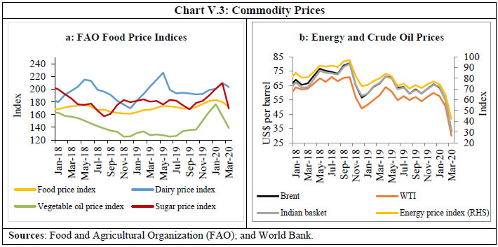 Base metal prices, measured by Bloomberg’s base metal index, fell by 17.9 per cent between October 2019 and March 2020 largely due to a demand slowdown. The firming of these prices during October-December on optimism over signing of the phase one trade deal between the US and China gave way to bearish sentiments from mid-January 2020. The spiralling of infected cases beyond Chinese borders and concerns about the global downturn intensified deflationary pressures pushing metal prices down (Chart V.4). Gold prices remained elevated in January-February, with prices rallying on safe haven demand amidst increased concerns over the global growth outlook (Box V.2). From mid-March, however, gold prices declined, falling below the US$ 1500 per troy ounce mark, on large sell-offs as investors fled to cash to compensate losses in other markets amidst heightened volatility. Box V.2: What Drives Gold Prices? As a financial asset, gold’s appeal typically rises in times of financial turmoil. Recently, growing concerns about a deep global slowdown due to COVID-19 boosted its safe haven demand. On year to date basis, gold prices shot up by 11 per cent (till March 09, 2020) on top of an 18 per cent increase in 2019 (Chart V.2.1a). Gold futures also traded higher (Chart V.2.1b). Through 2019, risk-off sentiments kept the overall appetite for gold strong as also evident in high exchange traded fund inflows, large purchases by central banks and increased COMEX net long positions. This upside to gold prices extended into 2020 up to mid-March as extreme risk aversion caused by COVID-19 sparked off sustained gold sales as it too lost allure amid heightened volatility, and gave way to an overriding preference to hold cash. This pulled down gold prices by 12 per cent between March 9 and 19, 2020. However, with subsequent recovery towards the end of March 2020, gold prices increased by 3.9 per cent on year to date basis (up to March 31, 2020). 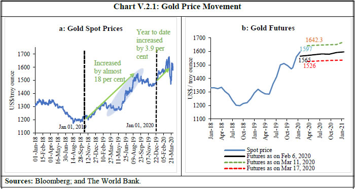 The empirical literature identifies a host of factors, viz., oil prices, global liquidity conditions, exchange rate, inflation, bond yields, stock prices and economic policy uncertainty as major drivers of gold prices. Investors consider gold as a tool for portfolio diversification, as it enables hedges against price risks of other financial instruments, and as a safe haven in times of economic and financial turmoil (Levin et al., 2006; Buar and Lucey, 2010; Emmrich and McGroarty, 2013; and Bilgin et al., 2018). The dynamics of gold prices are examined on a Johansen’s cointegration framework to estimate the long-run relationship. Gold prices (LGOLD), the US general price index (LCPIUS) and the US real exchange rate (LREERUS) are of one order of integration or I(1) and hence a long-run relationship between them could exist, as borne out by tests for cointegration. The estimated long-run equation is as follows: Equation (1) is augmented with the error correction term to capture the short-run dynamics of gold prices, while controlling for exogenous factors, viz., global economic policy uncertainty (EPU) index4, flight to safety proxied by changes in the Standard and Poor’s Index of US equity markets (ΔLS&P) and changes in Brent spot prices (ΔLOIL). The empirical analysis used monthly data for the period spanning January 2005 to December 2019. All the data, barring LCPIUS, were sourced from Bloomberg. LCPIUS was sourced from the website of the Federal Reserve of St. Louis. The short-run equation was estimated by adjusting for ARCH effects, since the errors were found to be heteroscedastic. Time dummies (October 2008 and May 2006) representing the periods of excessive intra-month volatility in gold prices were included (Table V.1.1). The error correction term turned out to be statistically significant with the correct negative sign. This indicates the return of the gold price to its long-run relationship and that the estimated model is stable. Δ LREERUS was found to be significant at one lag with a negative sign. This suggests that a depreciation in the US dollar would make gold cheaper outside the US dollar area leading to higher demand for gold and increase in gold prices in US dollar terms. Δ LCPIUS has negative relationship with gold prices in the short-run, which implies that a higher inflation in the US could dampen the demand for gold and reduce its price. This could be attributed to a host of factors, viz., central bank policies, investors’ preference to hold cash ahead of a recession and uncertainty perturbing the long-run relationship. The other variables, viz., economic and political uncertainty, stock index and crude oil prices had their expected signs and were statistically significant. 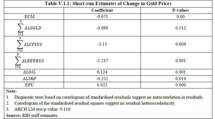 In sum, the empirical findings suggest that a rise in crude oil prices and a depreciation of the US dollar in the short-run lead to increase in gold prices. On the other hand, gold prices fall with a rise in equity prices. Gold prices also move in tandem with heightened economic policy uncertainty, thereby indicating the safe haven feature of the asset. References: Baur, D. G. and B. M. Lucey (2010), “Is Gold a Hedge or a Safe Haven? An Analysis of Stocks, Bonds and Gold”, The Financial Review, 45, 2, pp. 217–229. Bilgin, M. H., G. Gozgor, C. K. Lau and X. Sheng (2018), “The Effects of Uncertainty Measures on the Price of Gold”, International Review of Financial Analysis, 58, pp.1-7.
https://doi.org/10.1016/j.irfa.2018.03.009 Emmrich, O. and F. McGroarty (2013), “Should Gold be Included in Institutional Investment Portfolios? Applied Financial Economics, 23, pp. 1553–1565. Levin, E. J., A. Montagnoli and R. E. Wright (2006), “Short-run and Long-run Determinants of the Price of Gold”, World Gold Council, Research Study No 32.
http://strathprints.strath.ac.uk/7215/1/strathprints007215.pdf. | Inflation remained broadly contained in major AEs, but picked up in key EMEs on firming food prices. In the US, CPI inflation picked up modestly beginning October on rising prices of health services and food, though eased marginally in February on falling travel and fuel prices amidst COVID-19 disruptions. In terms of changes in the core personal consumption expenditure (PCE) deflator – the Fed’s preferred measure – inflation remained below the Fed’s 2 per cent target. In the Euro area too, inflation remained below target. Although energy and food inflation firmed up, measures of underlying inflation remained generally muted. Moreover, CPI inflation eased further in March on sharp decline in energy prices. In Japan, CPI inflation remained at a low level and edged down further in February on soft food prices and declining fuel prices (Chart V.5a). Inflation edged up across major EMEs, except Russia. China experienced persisting inflationary pressures on account of surging pork prices, which got accentuated in January due to seasonal demand during the lunar new-year holiday. However, inflation moderated slightly in February on easing non-food prices. In Brazil, CPI inflation has been rising since November on the back of strong gains in food prices, especially meat and transport prices, although falling food and beverages prices provided some relief in February. In South Africa, inflation increased for the third consecutive month in February, primarily driven by a rise in prices of food, non-alcoholic beverages and health services. CPI inflation eased in Russia, falling below the 4 per cent target from October 2019. Subdued external demand, falling food prices amidst excess supply and strong base effect related to the VAT rate hike a year ago exacerbated the downtrend. However, it increased marginally in March on firming services and non-food prices (Chart V.5b). 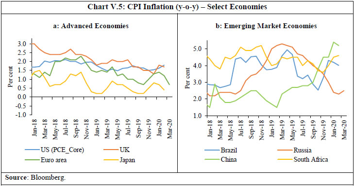 V.3 Monetary Policy Stance In 2019, monetary policy was said5 to have been the most accommodative across the world since the GFC. Most AEs as also some EMEs, kept their policy rate on hold in Q4:2019, but resorted to massive easing through both conventional and unconventional measures with the outbreak and rapid spread of COVID-19 in Q1:2020. The US Fed, which had paused in two consecutive FOMC meetings in December 2019 and January 2020, resorted to emergency rate cuts – 50 bps on March 3 and 100 bps on March 15 (Chart V.6a). With these sharp reductions, the Fed brought down the target range for the Federal Funds rate to the same level as during the GFC. The Fed has also announced several other measures such as asset purchases needed to support smooth market functioning and effective transmission of monetary policy, including commercial mortgage-backed securities in its purchase programme, lowering of the interest rate on primary credit to the same level as the top of the target range of the Federal Funds rate, allowing banks to use capital and liquidity buffers for lending, and reducing the reserve requirement to zero. The Fed has also launched dedicated facilities for financing support to commercial paper, primary dealers and money market mutual funds, while reviving the Term Asset-Backed Securities Loan Facility from the crisis time. The Fed would also be supporting credit to large employers, under new programmes. Besides, the Fed has also expanded dollar liquidity swap lines with other central banks and set up a temporary repo facility for foreign and international monetary authorities. The European Central Bank (ECB), has not changed key rates since a 10 bps reduction in deposit rate announced in its September 2019 meeting. In its March 2020 meeting, however, the ECB announced an additional €120 billion of net asset purchases, temporary longer-term refinancing operations and more favourable terms and quantum for the targeted longer-term refinancing operations (TLTRO) III for one year from June 2020. The ECB also announced a new €750 billion Pandemic Emergency Purchase Programme (PEPP) under which private and public sector securities would be purchased until end-2020 with flexibility on purchase flows over time, and across asset classes and jurisdictions, including Greek government bonds. The ECB also included non-financial commercial paper as eligible assets for its corporate sector purchase programme, and eased collateral requirements for its refinancing operations. The Bank of England (BoE), which was on a pause after raising the Bank rate in August 2018, undertook two out-of-turn rate cuts in March – of 50 bps and 15 bps – thereby reducing the Bank rate to an all-time low of 0.1 per cent. The BoE also announced additional asset purchases of £200 billion to be completed quickly in 2020. The BoE also announced macro-prudential relaxations and other incentives in order to support the economy with funds to tackle COVID-19 repercussions. The Bank of Canada (BoC), which was on a pause after October 2018, cut its policy rate by a cumulative 150 bps in March 2020, in three steps of 50 bps each to 0.25 per cent, to provide support to the Canadian financial system and the economy during the COVID-19 pandemic. The BoC has also introduced new liquidity support measures, including launching a quantitative easing programme. The Bank of Japan announced an enhancement of monetary easing in March 2020. The Reserve Bank of Australia (RBA), which was on a pause from November 2019 after having reduced the cash rate to an all-time low in October, reduced the cash rate by 25 bps each on two occasions in March to a new low of 0.25 per cent. The RBA also undertook additional measures such as yield curve control to be achieved through bond purchases, term funding facility and remuneration of exchange settlement balances of banks. The Reserve Bank of New Zealand undertook an emergency rate cut of 75 bps in March, pushing the policy rate to a new low of 0.25 per cent, besides announcing purchases under open market operations and other measures to support smooth functioning of the market. The Bank of Korea, on a pause since November 2019, undertook an emergency rate cut of 50 bps in March 2020 and announced other measures to stabilise economic and financial conditions. Riksbank was one of the few central banks that raised policy rates in 2019 with a hike of 25 bps in December 2019, thereby moving out of negative policy rate territory. In an emergency monetary policy meeting in March, however, the Riksbank announced additional asset purchases of SEK 300 billion, besides offering increased funding to banks on favourable terms and other measures. 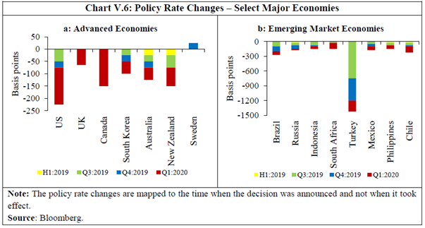 EMEs have also undertaken monetary easing and announced other liquidity support measures. The People’s Bank of China (PBoC) had effected a 5 bps cut in the one-year Loan Prime Rate (LPR) in November and followed it up with another 10 bps reduction in February 2020. The PBoC also injected about 1.2 trillion Chinese yuan of liquidity when markets opened on February 3 after an extended lunar new year break. It also announced a low-cost refinancing facility aimed at small and medium sized enterprises. In March, the PBoC lowered the reserve ratios for certain categories of banks and lowered the 7-day reverse repo rate by 20 bps. Other BRICS central banks remained in accommodative mode. The central bank of Brazil, which has been following ‘stimulative monetary policy’ and reducing the Selic rate since August 2019, cut this rate further by 50 bps each on two occasions in Q4:2019, and followed up with a 25 bps cut in February and a 50 bps cut in March. The Bank has also offered regulatory relaxations and other liquidity support facilities. The Bank of Russia, which had been reducing its policy rate in every policy meeting since June 2019, cut it by 25 bps each in its October, December and February meetings, but maintained a pause in the March meeting. The South African Reserve Bank, which had cut policy rate in July 2019 and had since maintained a pause, reduced its repo rate by 25 bps in January 2020 and a further 100 bps in March 2020 as the South African economy was expected to contract in 2020, having entered a recession in H2:2019 while inflation remained moderate (Chart V.6b). The central bank of Turkey, which embarked on policy accommodation in July 2019, cumulatively cut the policy rate by 675 bps on five occasions since October 2019. Banco de México, which cut its policy rate by 25 bps in each of its meeting since August 2019 as growth stagnated for several quarters, effected a 50 bps cut in March. The central bank of Philippines and Bank Indonesia, which were on pause after cutting rates in September, cut their policy rates by 25 bps each in February 2020, and by 50 bps and 25 bps, respectively, in March to support growth. Other central banks that cut rates on COVID-19 concerns include, inter alia, the Bank of Thailand, the Bank Negara Malaysia and the Central Bank of Chile. V.4 Global Financial Markets Global financial markets witnessed firming up of risk-on sentiment in Q4:2019 as a host of factors that had kept markets on edge – notably, the US-China trade tensions; and uncertainty regarding Brexit – receded to an extent. There was a bout of risk-off sentiment in early January due to geopolitical tensions emanating from the US-Iran conflict. However, calm quickly returned but when China declared on January 20 that there had been cases of human to human transmission of the novel coronavirus, sentiments turned extremely volatile, exacerbated by disagreement on oil production cuts between OPEC and Russia in March. In the same week, the WHO categorised the COVID-19 as a pandemic, which led to a tailspin in the markets and financing conditions tightened worldwide. Among AEs, US equities were on a continuous uptrend in Q4:2019, as the US Fed cut rates in October while the unemployment level in the US remained at a historic low. Positive news on the trade front – passing of the US-Mexico-Canada agreement by the House of Representatives and the announcement of the phase one agreement between the US and China – buoyed markets. In January, escalation of tension with Iran pulled down equities for a brief period. Another slide occurred after the outbreak of COVID-19. As China took strong action to restrict the limit and impact of COVID-19, US equities began rising again, reaching all-time highs in the third week of February. Immediately thereafter, with the rapid spread of COVID-19 to Italy, South Korea and Iran, sentiments worsened and the US indices registered their worst weekly performance since the GFC. The US Fed issued a statement that it stood ready to support the economy and announced an out-of-turn rate cut, which led to a recovery in the market for a couple of days. After the fallout between Russia and Saudi Arabia on crude oil and COVID-19 being declared a pandemic, the US equity market hit circuit breakers on two days in one week (March 9 and 12) – March 12 was the worst trading day since the Black Monday crash of October 19, 1987. The markets hit a circuit breaker again on March 16, just after the second emergency rate cut by the Fed. The marginal recovery in the latter part of March was on account of economic stimulus package worth about US$ 2 trillion being signed into law. In the UK and the Euro area, equity markets gained strength from December onwards with the UK general elections and certainty about Brexit. In Japan, stocks rose in Q4:2019 on expectation of higher profitability with favourable currency movement even as overall growth remained sluggish. With the COVID-19 outbreak, however, their indices crashed in sync with stock markets worldwide. Stock markets in EMEs mirrored this pattern. Driven by risk-on sentiments, stock markets in most EMEs registered handsome gains in Q4:2019 (Chart V.7). In Q1:2020, EME stock markets have been driven mainly by concerns about COVID-19, with additional headwinds arising from the crude oil price war in March. Chinese stocks fell most on February 3 after an extended lunar break. Other EME markets suffered sharper slides with frequent trading curbs in the second week of March. 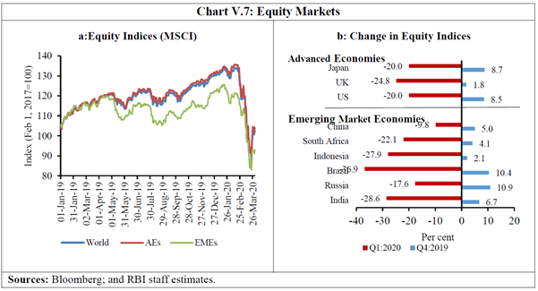 Bond yields firmed up across major AEs in the wake of risk-on sentiments, as also on improving global growth outlook and receding trade tensions in Q4:2019. With COVID-19, yields dipped on strong safe haven demand. In the US, the 10-year yield fell to historic lows in the fourth week of February as stock markets fell and demand for government bonds soared exemplifying flight to quality with the rapid spread of COVID-19 outside China and the US Centers for Disease Control and Prevention warning of increased risk to US residents. Yields dived below one per cent after the first emergency rate cut by the Fed, reaching an all-time low on March 9, before recovering marginally (Chart V.8a). Similar rallies were seen in bonds in other AEs, with yields reaching new lows in the UK and the Euro area. Bond yields across AEs continued to dip up to March 9, but increased sharply thereafter, with 10-year Japanese yields turning positive. Yields in EMEs, in general, softened in Q4:2019 with search for yield driving rates down. However, yields broadly remained range-bound up to February, but sharp risk-off sentiment in March led to a rout and yields across these economies rose sharply. 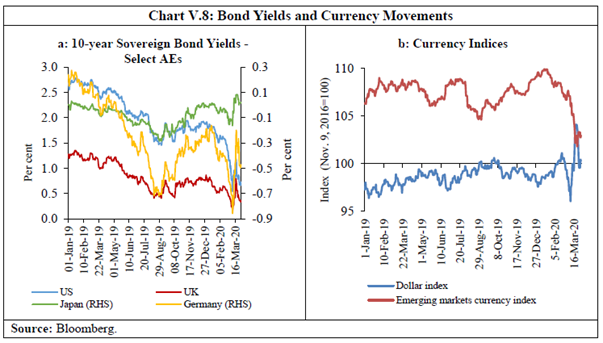 In currency markets, the US dollar weakened against major currencies, with the policy rate reduction by the Fed in October and guidance that it would pause. The dollar recovered in January with receding of trade tensions. With COVID-19, safe haven demand pushed up the dollar index further. However, with the virus spreading to the US and rising fatalities, as well as the rate cut by the Fed, the dollar weakened in early March (Chart V.8b). Most emerging market currencies, which had strengthened due to risk-on sentiment towards end-2019, weakened sharply with flight to safety in Q1:2020. The MSCI Emerging Market Currency Index increased by 3.6 per cent in Q4:2019 and declined by 6.0 per cent in Q1:2020. V.5 Conclusion In sum, global growth prospects have been rendered askew by COVID-19, with the near-term outlook extremely weak. Inflation in AEs remains benign, and a sharp decline in non-food commodity prices has imparted a further downward bias. Inflation concerns, however, remain in some EMEs although considerable uncertainty clouds the inflation outlook in the context of COVID-19. Global financial markets have become extremely volatile. Quick and coordinated actions by monetary authorities and governments have been taken, but there is little evidence as yet that they could mitigate the risks to the global economy from amplifying. _____________________________________________________________________________
ABBREVIATIONS | ACM | Adrian, Crump and Moench | | ADB | Asian Development Bank | | AE | Advance Estimates | | AEs | Advanced Economies | | AL | Agricultural Labourers | | AMCs | Asset Management Companies | | ANFC | Adjusted Non-Food Bank Credit | | APEDA | Agricultural and Processed Food Products Export Development Authority | | ARCH | Autoregressive Conditional Heteroscedasticity | | ARCH-LM | Autoregressive Conditional Heteroscedasticity - Lagrange Multiplier | | BK | Baxter-King | | BE | Budget Estimates | | BIS | Bank for International Settlements | | BoC | Bank of Canada | | BoE | Bank of England | | BoJ | Bank of Japan | | BoM | Bureau of Meteorology | | Bps | Basis Points | | BRICS | Brazil, Russia, India, China and South Africa | | BS | Bharat Stage | | CAD | Current Account Deficit | | CBLO | Collateralised Borrowing and Lending Obligation | | CCIL | Clearing Corporation of India Limited | | CD | Certificate of Deposit | | CDS | Credit Default Swap | | CF | Christiano-Fitzgerald | | CiC | Currency in Circulation | | CII | Confederation of Indian Industry | | CLI | Composite Leading Indicator | | CMBs | Cash Management Bills | | COMEX | Commodity Exchange | | COVID-19 | Coronavirus Disease 2019 | | CP | Commercial Paper | | CPB | Central Planning Bureau | | CPC | Central Pay Commission | | CPI | Consumer Price Index | | CPI-AL | Consumer Price Index for Agricultural Labourers | | CPI-IW | Consumer Price Index for Industrial Workers | | CPI-RL | Consumer Price Index for Rural Labourers | | CRAR | Capital to Risk Weighted Assets Ratio | | CRR | Cash Reserve Ratio | | CU | Capacity Utilisation | | CU (SA) | Capacity Utilisation (Seasonally Adjusted) | | DCA | Department of Consumer Affairs | | DGCA | Directorate General of Civil Aviation | | DGCI&S | Directorate General of Commercial Intelligence and Statistics | | ECB | European Central Bank | | ECBs | External Commercial Borrowings | | ECM | Error Correction Model | | EMEs | Emerging Market Economies | | e-NAM | National Agriculture Market | | ENSO | El Nino – Southern Oscillation | | EPU | Economic Policy Uncertainty | | ETF | Exchange Traded Fund | | EU | European Union | | FAO | Food and Agriculture Organisation | | FBIL | Financial Benchmarks India Pvt. Ltd | | FDI | Foreign Direct Investment | | FIs | Financial Institutions | | FICCI | Federation of Indian Chambers of Commerce and Industry | | FIMA | Foreign and International Monetary Authorities | | FIMMDA | Fixed Income Money Market and Derivatives Association of India | | FOMC | Federal Open Market Committee | | FPAS | Forecasting and Policy Analysis System | | FPI | Foreign Portfolio Investor | | FRBM | Fiscal Responsibility and Budget Management | | FRE | First Revised Estimates | | F-TRAC | FIMMDA Trade Reporting and Confirmation System | | GDP | Gross Domestic Product | | GDS | Gross Domestic Saving | | GEPU | Global Economic Policy Uncertainty Index | | GFC | Global Financial Crisis | | GFCE | Government Final Consumption Expenditure | | GFCF | Gross Fixed Capital Formation | | GFD | Gross Fiscal Deficit | | GNDI | Gross National Disposable Income | | GoI | Government of India | | GSDP | Gross State Domestic Product | | G-Secs | Government Securities | | GST | Goods and Services Tax | | GVA | Gross Value Added | | H1 | First Half of the Year | | H2 | Second Half of the Year | | HAC | Heteroscedasticity and Autocorrelation Consistent | | HP | Hodrick-Prescott | | HTM | Held to Maturity | | IIP | Index of Industrial Production | | IL&FS | Infrastructure Leasing & Financial Services Limited | | IMF | International Monetary Fund | | INR | Indian Rupee | | IOCL | Indian Oil Corporation Limited | | IOS | Industrial Outlook Survey | | ISM | Institute for Supply Management | | J-REIT | Japan Real Estate Investment Trust | | LAF | Liquidity Adjustment Facility | | LB | Ljung-Box | | LPG | Liquefied Petroleum Gas | | LPR | Loan Prime Rate | | LTROs | Long Term Repo Operations /Longer-term Refinancing Operations | | MCLR | Marginal Cost of Funds Based Lending Rate | | MEP | Minimum Export Price | | MFs | Mutual Funds | | MGNREGA | Mahatma Gandhi National Rural Employment Guarantee Act | | MIBOR | Mumbai Interbank Outright Rate | | MMRP | Modified Mixed Reference Period | | MOAFW | Ministry of Agriculture and Farmers Welfare | | m-o-m | Month-on-Month | | MPC | Monetary Policy Committee | | MPR | Monetary Policy Report | | MS | Mild Steel | | MSCI | Morgan Stanley Capital International | | MSF | Marginal Standing Facility | | MSME | Micro, Small and Medium Enterprises | | MSP | Minimum Support Price | | MVKF | Multivariate Kalman Filter | | NAV | Net Asset Value | | NBFCs | Non-Banking Financial Companies | | NCAER | National Council of Applied Economic Research | | NDS-OM | Negotiated Dealing System-Order Matching | | NDTL | Net Demand and Time Liabilities | | NEER | Nominal Effective Exchange Rate | | NGNF | Non-Government Non-Financial | | NLP | Natural Language Processing | | NOAA | National Oceanic and Atmospheric Administration | | NPA | Non-Performing Asset | | NSC | National Savings Certificate | | NSDL | National Securities Depository Limited | | NSE | National Stock Exchange | | NSO | National Statistical Office | | NSSO | National Sample Survey Office | | OD | Overdraft | | OECD | Organisation for Economic Cooperation and Development | | OIS | Overnight Indexed Swap | | OLS | Ordinary Least Squares | | OMCs | Oil Marketing Companies | | OMOs | Open Market Operations | | OPEC | Organisation of the Petroleum Exporting Countries | | OTC | Over-the-Counter | | PADO | Public Administration, Defence and Other services | | PBoC | People’s Bank of China | | PCE | Personal Consumption Expenditure | | PDS | Public Distribution System | | PEPP | Pandemic Emergency Purchase Programme | | PFCE | Private Final Consumption Expenditure | | PLFS | Periodic Labour Force Survey | | PMI | Purchasing Managers’ Index | | POL | Petroleum, Oil and Lubricants | | PSBs | Public Sector Banks | | PSU | Public Sector Undertaking | | Q1 | First Quarter | | Q2 | Second Quarter | | Q3 | Third Quarter | | Q4 | Fourth Quarter | | q-o-q | Quarter-on-Quarter | | QPM | Quarterly Projection Model | | RBA | Reserve Bank of Australia | | RBI | Reserve Bank of India | | RE | Revised Estimates | | REER | Real Effective Exchange Rate | | RHS | Right Hand Side | | RL | Rural Labourers | | SAAR | Seasonally Adjusted Annualised Growth Rate | | SAE | Second Advanced Estimates | | SCBs | Scheduled Commercial Banks | | SDLs | State Development Loans | | SEBI | Securities and Exchange Board of India | | SI | Sentiment Index | | SIAM | Society of Indian Automobile Manufacturers | | SLR | Statutory Liquidity Ratio | | SPDs | Standalone Primary Dealers | | SSTs | Sea Surface Temperatures | | T-Bill | Treasury Bill | | TLTRO | Targeted Longer-term Refinancing Operations | | ToT | Terms of Trade | | UK | United Kingdom | | US | United States | | US$ | US Dollar | | VAR | Vector Autoregression | | VAT | Value Added Tax | | WAC | Weighted Average Coupon | | WACR | Weighted Average Call Money Rate | | WADR | Weighted Average Discount Rate | | WADTDR | Weighted Average Domestic Term Deposit Rate | | WALR | Weighted Average Lending Rate | | WAM | Weighted Average Maturity | | WHO | World Health Organisation | | WMA | Ways and Means Advances | | WPI | Wholesale Price Index | | WTI | West Texas Intermediate | | WTO | World Trade Organisation | | y-o-y | Year-on-Year | |