|
Abstract: Some Indian states have announced farm debt waivers recently, which bear ramifications for the fiscal burden of states over the medium term. Empirical estimates suggest that fiscal deficit can have an inflationary impact. In particular, impact is non-linear as fiscal deficit causes inflation to rise more at higher level of fiscal deficit and inflation. If the combined fiscal deficit for 2017-18 goes up by 40 bps on account of farm loan waivers(both actual and intended), with the budgeted combined fiscal deficit at around 5.9 percent for 2017-18 and inflationary momentum remaining benign, ceteris paribus, this may lead to around 20 bps permanent increase in inflation, starting 2017-18.
In India, farm loan waivers have been announced intermittently by both the central and state governments to provide relief to farmers facing distress due to natural calamities / crop failure. Recent instances of such waivers include the Agricultural Debt Waiver and Debt Relief (ADWDR) Scheme announced by the central government in 2008 and state-specific farm loan waivers announced by Andhra Pradesh and Telangana in 2014; Tamil Nadu in 2016; and Uttar Pradesh (UP), Maharashtra, Punjab and Karnataka in 2017 (so far).
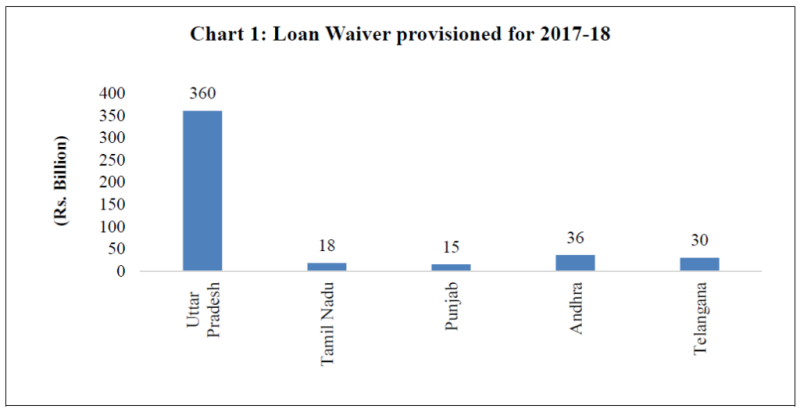
In April 2017, UP announced a farm loan waiver scheme, which is expected to benefit small and marginal farmers by writing off their loans to the tune of ₹ 360 billion – around 2.5 per cent of UP’s Gross State Domestic Product (GSDP). Maharashtra has since announced a loan waiver scheme for farmers amounting to ₹ 340 billion. Similarly, Punjab has announced a waiver on crop loans benefitting small and marginal farmers (for which a provision of ₹ 15 billion has been made in the state budget for 2017-18) while Karnataka has announced a loan waiver amounting to ₹ 81.65 billion for farmers availing of farm loans from cooperative banks. Most of these states have factored in the expenditure towards loan waiver in their respective state budgets with the exception of Maharashtra and Karnataka, which announced loan waivers post their budget presentation (Chart 1). Apart from these states, several others are contemplating loan waivers with the intended waiver amounts ranging between ₹400 - ₹570 billion.2
 Loan waivers could add to the fiscal burden over the medium term as they are essentially a transfer from tax payers to borrowers.3 Based on stylized assumptions, the total loan waiver amount that is likely to be released in 2017-18 by seven states is around ₹881 billion (0.5 per cent of Gross Domestic Product, GDP). Depending on possible sources of financing, the additional burden including (i) additional market borrowing and (ii) pruning of wasteful expenditure, this may result in an increase in the consolidated Gross Fiscal Deficit - Gross Domestic Product (GFD-GDP) ratio of the states by about 20-40 basis points (bps).4 Higher fiscal deficits per se can lead to an increase in inflation expectations and actual inflation.5
It is also pertinent to note that random fiscal policy shocks, such as loan waivers, have an enduring impact on market borrowings, as evident from past episodes of such waivers. If overall government borrowing increases, yields on state development loans (SDL) may firm up posing higher interest burden for the states in future. Concomitantly, they can also crowd out private borrowers as the general cost of borrowing increases with pressure from higher government borrowing on the finite pool of investible resources in the economy. Thus, state government farm loan waivers have the potential to crowd out corporate borrowings if financed through SDL issuance.
We examine the short-run as well as long-run impact of combined GFD to GDP ratio on CPI inflation by incorporating the possible non-linearities of the impact of fiscal deficit on inflation.
Let us define X = Combined Fiscal Deficit (GFD)/Nominal GDP and Π = Consumer Price Index (CPI) inflation. For accommodating the non-linear impact, X is transformed as X1 = (X2)/2; and Π1 = Log (1+ Π). The long-run relationship is defined as Π1 = a+b*X1 and we are interested in estimating dΠ /dX = b* X* (1+ Π). These transformations allow for the inflation-fiscal deficit elasticity to change across different inflation and fiscal deficit levels. The long-run-relationship and direction of causality are tested using the Auto Regressive Distributed Lag (ARDL) cointegration approach, also known as bounds test.6 Analysis is done using quarterly data from Q2:2006-07 to Q3:2016-17. The quarterly combined deficit figures of center and all states (GFD-C) are not available as the corresponding data for states are not obtainable at a quarterly frequency. Therefore, we have used the quarterly fiscal deficit numbers of the centre as the proxy variable to interpolate the annual combined fiscal deficit using the proportional Denton method.7
 The choice of the number of lags of the dependent and the independent variables is based on the overall model properties and the regression diagnostics. The results of the bounds test with Π1 as the dependent variable (equation 1) and with X1 as the dependent variable (equation 2) are given in Table 1. With Π1 as the dependent variable, the F statistic is above the upper bound of the critical value at 1 per cent level, suggesting that the null hypothesis of no cointegration is rejected. While with X1 as the dependent variable, the F statistic is below the lower bound of the critical value indicating no cointegration. These results indicate that inflation, in the long-run, is significantly influenced by combined fiscal deficit.
| Table 1: ARDL Bounds Test for Cointegration |
| Dependent Variable |
F statistic |
Critical Values at 1% with 40 observations, 2 regressors with intercept and no trend |
| Π1 |
7.95 |
[5.893, 7.337] |
| X1 |
4.78 |
[5.893, 7.337] |
The short-run regression equations suggest that the error correction term, changes in fiscal deficit and crude oil prices significantly affect the changes in inflation. The regression diagnostics of no autocorrelation and homoscedasticity in errors are found to be satisfactory.9 The significance of long-run relation (in Table 1) and robustness of the short-run equation suggest that the long-run equation of inflation on fiscal deficit can be derived as
 The slope coefficient dΠ1/dX1 is 0.017, which is the change in Π1 (which is log(1+ Π)) when X1 (which is = (X2)/2) changes by one unit. However, the coefficient of our interest is the change in inflation (Π) when fiscal deficit (X) changes by one unit, which can be deducted as 0.017*(1+ Π)*X. This shows that the change in inflation induced by a unit change in fiscal deficit is dependent on both the level of inflation as well as the level of fiscal deficit. In other words, this indicates that at higher levels of inflation and fiscal deficit, the impact of fiscal deficit on inflation will be higher.
Equation 3 can be used to estimate the impact of one per cent increase in GFD-C on CPI inflation (in bps) at different levels of inflation and fiscal deficit (Chart 2).
The empirical results suggest that there exists a positive and statistically significant long-run relation leading from fiscal deficits to inflation in India which is non-linear in nature, i.e., the impact of fiscal deficit on inflation will be higher at higher levels of the fiscal deficit and inflation. To summarise, if the combined fiscal deficit for 2017-18 goes up by 40 bps on account of farm loan waivers, with the budgeted combined fiscal deficit at 5.9 percent for 2017-18 and inflationary momentum remaining benign, ceteris paribus, this may lead to around 20 bps permanent increase in inflation, starting 2017-18.
References:
Catao, L. A., and M. E. Terrones (2005). Fiscal deficits and inflation. Journal of Monetary Economics, 52(3), 529-554.
Leeper, E. M. (1991). Equilibria under ‘active’ and ‘passive’ monetary and fiscal policies. Journal of Monetary Economics, 27(1), 129-147.
Narayan, P. K. (2005). The saving and investment nexus for China: evidence from cointegration tests. Applied economics, 37(17), 1979-1990.
Pesaran, M. H., Y. Shin, and R.J. Smith (2001). Bounds testing approaches to the analysis of level relationships. Journal of Applied Econometrics, 16(3), 289-326.
Sargent, T. J. and N. Wallace (1981). Some unpleasant monetarist arithmetic. Federal Reserve Bank of Minneapolis Quarterly Review, 5(3), 1-17.
Reserve Bank of India (2012). Report of the Expert Committee to Revise and Strengthen the Monetary Policy Framework, Available at https://rbidocs.rbi.org.in/rdocs/PublicationReport/Pdfs/ECOMRF210114_F.pdf
|