by Srijashree Sardar, Dipak R. Chaudhari, Priyanka Priyadarshini, Anshul and Sangeeta Das^ This article examines the impact of movements in the real effective exchange rate (REER) on India’s merchandise trade balance using a non-linear autoregressive distributed lag (NARDL) model. The empirical findings suggest that depreciation in REER improves trade balance while appreciation deteriorates it. The impact of REER depreciation on trade balance is more than an equivalent REER appreciation in the short-run and vice versa in the long-run. Cross-country estimates indicate that the REER is influenced by productivity differential, terms of trade, government expenditure and net foreign assets. Introduction Exchange rate is one of the indicators impacting country’s external competitiveness. One issue in this regard is as to whether the real exchange rate (RER) is a useful measure for this purpose. The nominal effective exchange rate (NEER) is a trade weighted average exchange rate of domestic currency in terms of a basket of foreign currencies, while the real effective exchange rate (REER) is an inflation-adjusted trade-weighted average value of the domestic currency in terms of its trading partners’ currencies. In the short-run, REER movements may primarily reflect changes in the nominal exchange rate, as prices are generally sticky in the short-run (Darvas, 2021). Although imperfect, REER fairly signals large overvaluation/undervaluation and makes it one of the early warning tools for policymakers (Cenedese and Stolper, 2012). The relationship between REER and trade balance can be ambiguous. In the trade channel, REER depreciation could be beneficial for net exports, while the finance channel can offset these benefits and can reduce GDP growth (BIS, 2018). Cardarelli and Rebucci (2007) found a stable link between REER and trade balances through expenditure switching channel; later studies suggest that the relationship could be asymmetric and non-linear. Currency depreciation can have a stronger effect on trade balance than currency appreciation of equal magnitude (Bahmani-Oskooee and Aftab, 2017; and Arize, 2017). There is evidence of J-curve effect – depreciation of REER may immediately worsen the trade balance with reversal over time, leading to improvement in trade balance. Bhat and Bhat (2021) found no evidence of J-curve phenomenon in the case of India; the authors found that appreciation deteriorates trade balance, while depreciation improves it in the short run. However, in the long run, only depreciation impacts trade balance. This indicates asymmetric impact of REER movements on trade balance. Parray, Wani and Yasmin (2022) using post liberalisation period also found no evidence of ‘J-curve’ effect and ‘Marshal-Lerner’ conditions in India. The study also indicated that among other macroeconomic variables, exchange rate is a highly influential factor in India’s trade balance. Against this background, Section II discusses approaches to equilibrium exchange rate (EER) estimation. Section III empirically estimates equilibrium real exchange rate for a panel of eight countries. Section IV provides an overview of REER estimation in India. Section V empirically examines asymmetric impact of REER on trade balance of India using non-linear autoregressive distributed lag model (NARDL), while section VI provides concluding observations. II. Approaches to Estimate Real Exchange Rate Conceptual Background for Estimating Real Exchange Rate A common equilibrium exchange rate approach focuses on deviations of the exchange rate from the Purchasing Power Parity (PPP) proposition, which postulates that the equilibrium exchange rate between two countries is determined by their respective purchasing powers, and, in turn, their inflation rates. Deviations from PPP imply that, q = s – (p - p*) = Ɛ ≠ 0 where q is the real exchange rate, s is the nominal exchange rate, and p and p* are the domestic and foreign prices respectively (all in log terms). Ɛ stands for factors that can explain the non-stationary movement of q. The Behavioural Equilibrium Exchange Rate (BEER) approach assumes a cointegrating relationship between q and Ɛ, yielding a reduced form estimation of the Equilibrium Real Exchange Rate (ERER). The acronym BEER is often used to indicate, by extension, a whole family of models that follow similar methodologies. Another approach calculates ERER as the one that satisfies both medium-term internal and external balances1 and is known as the Fundamental Equilibrium Exchange Rate (FEER). In a recent study, Patra et al. (2024) devise a suite of approaches for estimating equilibrium exchange rates for India and state that the alternative approaches are preferable to static indicators such as the REER or others that belong in the genre of the simple PPP framework. REER in emerging economies is mainly driven by economic fundamentals, interest rate differential and terms of trade (Raut, 2021). Clark and MacDonald (1999) found that BEER, in the long run, is determined by terms of trade, relative price of non-traded to traded goods, the stock of net foreign assets and interest rate differential. According to Clark and MacDonald (op. cit.), both the FEER and BEER approaches have strengths and weaknesses: The BEER approach provides a direct estimate of misalignment and is useful for short-term analysis, subject to the risk of model misspecification; conversely, the FEER approach is more robust but relies heavily on the assumptions of full employment and capital account sustainability. The equilibrium REER depends, inter alia, upon - i) Net Foreign Assets: debtor countries (foreign liabilities exceeding foreign assets), ceteris paribus, need a more depreciated real exchange rate to generate trade surpluses necessary to service their external liabilities; ii) Productivity Differential: higher productivity is related to appreciation in REER; iii) Terms of Trade: favourable terms of trade can appreciate the REER through income or wealth effects; and iv) Government Consumption: higher government consumption is associated with the appreciation of REER as such consumption is mostly related with non-tradable sector than tradable sector leading to higher relative prices (Lee et al., 2008). Estimation of REER in Practice In practice, REER computation needs to account for four major components: the range of foreign trading partners, their relative weights, the price indices and choice of base year. International organisations, including BIS, OECD, World Bank and IMF publish REERs for different countries. These databases employ different computation methodologies, country, and currency composition, thereby yielding different figures for the REER. The US Federal Reserve compiles six types of REER indices based on different country weights on a monthly frequency.2 The Bank of England currently calculates the Sterling exchange rate index at daily, monthly and quarterly frequencies.3 A broader currency index provides a global picture by taking a large number of currencies, while a smaller index gauges competitiveness over advanced economies (Fung et al., 2006). The preferred index could depend on the context of the study (Klau and Fung, 2006). III. Equilibrium Real Exchange Rate: Cross Country Analysis To understand the potential determinants of REER, a panel regression empirical exercise is carried out in this section covering the following countries: India, Brazil, China, Indonesia, Malaysia, Russia, South Korea and Thailand, with annual data of 27 years- 1994 to 2021. As discussed in the previous section, the CPI-based REER is expected to be determined by the following four fundamentals in the long run: Net foreign assets (NFA), productivity differential, commodity terms of trade (ToT) and government consumption expenditure. NFA data has been sourced from Lane and Milesi-Ferretti (2018), database. Productivity differential is obtained as real per capita GDP of a country vis-à-vis its 64 trading partners multiplied by their corresponding trade weights. GDP data is sourced from the World Bank and trade weights data have been sourced from BIS. Commodity terms of trade (ToT) was estimated in line with Gruss and Kebhaj (2019) - log of terms of trade index (June 2012=100) which is the commodity net export price index (weighted by net exports to total commodity trade). Data on government consumption expenditure as a ratio of GDP (GEXPR/GDP) was sourced from World Bank. Panel unit root test (Levin et al., 2002) results depict that all the variables are first difference stationary (Table 1). | Table 1: Results of Panel Unit Root Tests | | Variable | Level | First Difference | | | LLC t-stat | LLC t-stat | | LREER | -1.55 | -9.11*** | | | (0.06) | (0.00) | | GEXPR/GDP | -1.54 | -4.16*** | | | (0.06) | (0.00) | | Productivity Differential | -1.21 | -3.39*** | | | (0.11) | (0.00) | | NFA/GDP | -0.43 | -4.99*** | | | (0.33) | (0.00) | | ToT | -1.68 | -7.29*** | | | (0.06) | (0.00) | Note: Figure in brackets are p-values; *** indicates statistical significance at 1 per cent.
Source: Authors’ estimates. |
| Table 2: DOLS Estimates of Long-run Cointegrating Relationship | | Variable | Coefficient | p-value | | Dependent variable: log of REER (LREER) | | GEXPR / GDP | 1.99*** | 0.00 | | | (4.24) | | | NFA / GDP | -0.16*** | 0.00 | | | (-4.99) | | | Productivity Differential | 1.74*** | 0.00 | | | (13.29) | | | ToT | 0.27*** | 0.00 | | | (7.81) | | | Adjusted R2 | 0.79 | | Observations | 184 | Note: Figure in brackets are t-statistics; *** indicates statistical significance at 1 per cent.
Source: Authors’ estimates. | Evidence of panel cointegration - long-run relationship between the LREER and the set of fundamentals - among the variables is indicated by the Kao (1999) test. The results of dynamic ordinary least squares (DOLS) methodology developed by Stock and Watson (1993) have been summarised in Table 2. The ERER approach does not provide the information on how quickly the exchange rate would adjust to restore equilibrium. Therefore, the long-run model was estimated with an error-correction specification. The results suggest that it takes approximately, on an average, four years to halve the gap between actual and equilibrium exchange rates for the selected countries and time period (Table 3). | Table 3: Error Correction Term Coefficient | | | Coefficient | p-value | | Error Correction Term | -0.12***
(-3.84) | 0.00 | Note: Figure in brackets are t-statistics; *** indicates statistical significance at 1 per cent.
Source: Authors’ estimates. | IV. REER Estimates for India The Reserve Bank of India (RBI) computes two REER indices - 40-currency (broad) and 6-currency (narrow) – representing 88 per cent (Guria and Sokal, 2021) and 40 per cent of India’s trade, respectively. The indices use 3-year moving geometric mean trade weights of India’s bilateral trade (exports plus imports) with partner countries (forty/six countries). This method suitably reflects the dynamically changing pattern of India’s foreign trade with its major trading partners. The 40-currency REER/NEER is available in two series - trade weighted and export weighted. The 6-currency is computed on trade weighted basis only; however, it is also available on rolling base year series, in addition to 2015-16 base year. A comparison of 40-currency and 6-currency REER / NEER indices indicates long-run co-movement (Chart 1). The transitory divergence in 40-currency and 6-currency REER during January 2021 to April 2022 was due to higher inflation in the rest of the countries (excluding 6-currency). The most commonly used price index in REER calculation is the consumer price index (CPI) as it is available timely (Ellis, 2001) [Chart 2]. In the 6-currency REER, USD and Chinese renminbi each have 28 per cent weight, Euro has 26 per cent, Hong Kong Dollar has 8 per cent, while UK pound and Japanese Yen have equal weights of 5 per cent each. Of these, five currencies are in global top five in terms of currency trade and central banks’ official reserves (Table 4).4 However, the USD still holds top share in central banks’ coffers. | Table 4: Global Top Five Currencies | | Rank | Currency | Share in OTC FX trading | Amount of currency trade daily (USD bn) | Share in Official Reserve composition | | 1 | USD | 88 | 6,641 | 58.36 | | 2 | EUR | 31 | 2,293 | 20.47 | | 3 | JPY | 17 | 1,253 | 5.51 | | 4 | GBP | 13 | 969 | 4.95 | | 5 | CNY | 7 | 526 | 2.69 | | Source: BIS Triennial Survey on Global Foreign Exchange Market, October 2022 and IMF, COFER dated March 31, 2023. | The select 6 currencies had a share of 43 per cent in India’s merchandise export and 37 per cent in merchandise import in 2021-22. The coverage of 6-currency REER and NEER in total trade increased from 33 per cent in 2012-13 to 43 per cent in 2020-21 before declining to 39 per cent in 2021-22 due to Covid led disruptions. The share of imports from these 6 economies has been increasing which may reflect concentration in merchandise imports due to product quality of intermediate inputs among others (Table 5). | Table 5: India’s Bilateral Merchandise Trade (Export + Import) Shares | | | 2017-18 | 2018-19 | 2019-20 | 2020-21 | 2021-22 | 5-years average | | China | 11.66 | 10.31 | 10.39 | 12.59 | 11.19 | 11.18 | | USA | 9.69 | 10.42 | 11.28 | 11.73 | 11.54 | 10.95 | | Eurozone | 10.17 | 10.72 | 10.41 | 10.66 | 10.13 | 10.40 | | UAE | 6.49 | 7.10 | 7.50 | 6.31 | 7.04 | 6.92 | | Saudi Arabia | 3.57 | 4.03 | 4.20 | 3.21 | 4.14 | 3.87 | | Hong Kong | 3.30 | 3.67 | 3.54 | 3.69 | 2.91 | 3.39 | | Singapore | 2.30 | 3.30 | 3.00 | 3.20 | 2.91 | 2.94 | | Iraq | 2.48 | 2.86 | 3.25 | 2.30 | 3.32 | 2.89 | | Korea Rp | 2.71 | 2.54 | 2.60 | 2.54 | 2.47 | 2.57 | | Indonesia | 2.65 | 2.50 | 2.44 | 2.55 | 2.53 | 2.53 | | Switzerland | 2.60 | 2.28 | 2.30 | 2.84 | 2.39 | 2.46 | | Japan | 2.04 | 2.09 | 2.15 | 2.24 | 1.99 | 2.09 | | Australia | 2.34 | 1.97 | 1.60 | 1.79 | 2.42 | 2.05 | | Malaysia | 1.91 | 2.04 | 2.05 | 2.10 | 1.88 | 1.99 | | UK | 1.89 | 2.00 | 1.96 | 1.91 | 1.69 | 1.88 | | Source: Directorate General of Commercial Intelligence and Statistics (DGCI&S); Authors’ calculation. | The Covid pandemic and protectionist trends have led to a change in direction as well as share of India’s trading partners in the past few years. India’s direction of exports has moved toward North America and Africa with the combined share increasing from 17.3 per cent in 2009-10 to 27 per cent in 2021-22 (Annex Chart 1A and 1B). The share of imports from Asia has increased from 28.6 per cent in 2009-10 to 36.6 per cent in 2021-22, mainly driven by China while the share of EU has declined from 13.3 per cent in 2009-10 to 8.4 per cent in 2021-22. Similarly, the composition of India’s current account has been changing over time with services exports gaining importance as compared to merchandise exports. The share of services exports in India’s total exports of goods and services increased from 31 per cent in 2011-12 to 44 per cent in 2023-24, while share of services in the total imports increased to 21 per cent from 13 per cent during the same period (Chart 3a and 3b). Further, the average services export growth of India at 14 per cent in the past 30 years (1993-2022) when world services export growth was only 4.3 per cent in 2022 indicates higher potential for skilled labour economies like India (Gajbhiye et al., 2024). In services exports, ‘telecommunication, computer and information services’ and ‘other business services’ dominate India’s exports. In this context, central banks in some economies like Bank of England and Reserve Bank of New Zealand also include trade in services in their REER compilation. However, data availability and quality of bilateral trade in services statistics are the main issues in getting services included in the REER compilation. As such, many institutions such as BIS, OECD and central banks, do not use services in the REER compilation (Klau and Fung, 2006). However, these limitations notwithstanding, the merchandise trade-based REER serves as a useful indicator of competitiveness.  Dominant Currency Paradigm The trade-weighted REER and NEER assume that the use of a country’s currency in world trade is closely tied to its share in world trade. In other words, depreciation of a country’s currency vis-à-vis all the trade partners increases the price of imports in domestic currency, making imports costlier and thus reducing demand for foreign goods. At the same time, it also reduces the price of exports in destination country leading to increase in exports. In this context, in the presence of “Dominant Currency Paradigm” - when trade is invoiced in the dominant country’s currency (viz. USD, Euro) regardless of the origin or destination of trade flows - the traditional expenditure switching effects could be weak (Boz et al., 2020; Gopinath, 2015). With the high share of trade invoiced in US dollar and Euro, the computation of REER based on trade shares may not fully capture the currency competitiveness. Boz et al. (op. cit.) find that USD exchange rate passthrough is higher vis-à-vis bilateral exchange rates in imports, for a country with higher share of trade invoicing in USD. Further, the paper also finds that depreciation of domestic currency with respect to USD in comparison to bilateral exchange rate leads to a greater decrease in trade volumes. V. Impact of REER on India’s Trade Balance: Empirical Analysis Literature in case of India reflects similar findings as was observed in the cross country analysis set out above (Ghosh et al., 2023; Raut, 2021). For the empirical analysis in this article, a set of five variables are used with quarterly frequency covering the period from April 2012 to June 2024. The dependent variable trade balance (TB) was in deficit throughout the period. The TB is expressed as the absolute figure of the difference between exports and imports i.e., |export-import|. The increase (decline) in TB indicates deterioration (improvement) in trade balance. This is also in line with the REER construction, as decline in REER reflects depreciation and improvement in trade balance (Bhat and Bhat, 2021). India’s GDP and OECD-GDP are taken as domestic demand and foreign demand, respectively. Both the 40-currency REER (broad index) and 6-currency REER (narrow index) are used in two separate models to understand the exchange rate dynamics. The geopolitical risk (GPR) index has been included in the models acknowledging adverse impact of geopolitical events on the international trade (Gajbhiye, et al., 2024). To account for seasonality, all the variables are transformed into seasonally adjusted quarterly series using X-13 ARIMA and then transformed into logarithmic scale. A Vector Error Correction Model (VECM) followed by a non-linear autoregressive distributed lag (NARDL) model has been used for 40-currency and 6-currency REER (base year 2015-16) to compare and examine the asymmetric relationship between trade balance and REER. Considering the asymmetric impact of REER on trade balance, the estimable function could be expressed in the form as follows: 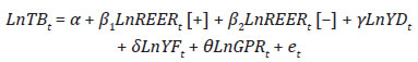 Here, the trade balance (TB) is determined by REER [+] (appreciation), REER [–] (depreciation), domestic demand (YD) and foreign demand (YF), geopolitical risk (GPR) and other factors (et). The ARDL cointegration technique is used to determine long-run relationship between the series with different order of integration (Pesaran and Shin, 1999, and Pesaran et al. 2001). The reparametrized result gives the short-run dynamics and long run relationship of the select variables. Here, the Johansen test is applied to estimate cointegrating relationship of TB with REER and India’s domestic demand and foreign demand. The sources and descriptive statistics of the variables under study have been given in Annex (Table 1A and 2A). In this case, the standard augmented Dickey-Fuller (ADF) unit root test and Phillips-Perron unit root test explain that no series under consideration is integrated of order 2 or higher order (Annex Table 3A) confirming suitability of variables for ARDL model. | Table 6: Result of Bounds Test | | Model | I(0) | I(1) | F-statistic | Status | | M1 (40-Currency REER) | 3.740 | 4.303 | 4.671 | Cointegrated | | M2 (6-Currency REER) | 3.777 | 4.320 | 4.982 | Cointegrated | Note: I(0) and I(1) are respectively the stationary and non-stationary bounds at 5 per cent significance level.
Source: Authors’ estimates. | Empirical Results: Cointegration Test The bounds test results for both the models considering regressors as 40-currency REER/6-currency REER confirm cointegration relationship among the select variables (Table 6). Symmetry Test Further, to explore the asymmetric relationship between TB and REER (both 40-currency and 6-currency), NARDL model has been employed. The coefficient symmetry test indicates the existence of long run and short run asymmetrical association between trade balance and REER for both broad and narrow indices (Table 7). Short run and long run relationship The short-run impact of variables on the trade balance highlights that except for foreign demand (GDP_OECD), all other coefficients of model M1 (40-currency REER) are statistically significant while in M2 (6-currency REER), all indicators are significant except foreign demand and 6-currency REER [+], i.e., the appreciation factor (Table 8). The significant negative coefficients of ΔlnYD in both models show that the expansion in India’s GDP worsens the trade balance in the short run since a productivity-driven increase in income may lead to a higher demand for imports. | Table 7: Coefficients Symmetry Test | | | Long-Run | Short-Run | | F-statistic | Probability | F-statistic | Probability | | M1 (with 40-Currency REER) | 11.487*** | 0.002 | 4.356** | 0.044 | | M2 (with 6-Currency REER) | 12.293*** | 0.001 | 7.431*** | 0.010 | Note: *** and ** denote significance at 1 per cent and 5 per cent levels.
Source: Authors’ estimates. | The results indicate that the effect of REER depreciation is significant for both the REER (broad and narrow) and stronger than REER appreciation, although appreciation is statistically insignificant for 6-currency REER. Thus, the relationship between these two variables is asymmetric, i.e., currency depreciation impacts the balance of trade more than an equivalent currency appreciation in the short-run, which is in line with other studies (Bhat and Bhat, 2021; Parray et al., 2022) and contrary to Raut (2021). The Error Correction terms (ECT) are negative with an associated coefficient estimate of -0.545 and -0.483, for 40-currency REER and 6-currency REER, respectively, and are highly significant. | Table 8: NARDL Error Correction Estimation-Short Run Coefficients | | | M1: 40-currency REER | M2: 6-currency REER | | Variables | Coefficient | P-value | Coefficient | P-value | | | -0.545*** | 0.000 | -0.483*** | 0.000 | | ECT | (0.127) | | (0.123) | | | | 0.393*** | 0.000 | 0.303*** | 0.001 | | ΔlnTBt-1 | (0.088) | | (0.080) | | | ΔlnYDt | -4.555*** | 0.001 | -4.262*** | 0.001 | | | (1.252) | | (1.209) | | | ΔlnYFt | -1.881 | 0.499 | -1.557 | 0.561 | | | (2.757) | | (2.655) | | | ΔlnREERt [+] | 3.583* | 0.101 | 2.442 | 0.219 | | | (2.425) | | (1.959) | | | ΔlnREERt [–] | -5.871*** | 0.003 | -5.460*** | 0.001 | | | (2.425) | | (1.534) | | | C | 30.021*** | 0.000 | 25.413*** | 0.000 | | | (6.998) | | (6.478) | | Note: ***, ** and * denote significance at 1 per cent, 5 per cent and 10 per cent level. . Figures in Parenthesis are standard errors.
Source: Authors’ estimates. | In the long-run, the asymmetric effect of REER changes – appreciation (+) and depreciation (–) – is also evident in model M1, although here the impact of currency appreciation is stronger than an equivalent currency depreciation in contrast to the short-run dynamics (Table 9). The rising productivity within the tradable goods sector has played a significant role in the sustained trend of appreciation in REER (Patra, et al., 2024). The foreign demand (YF) is also statistically significant with expected signs indicating that increase in foreign demand leads to increase in India’s exports demand and improves trade balance. | Table 9: NARDL - Long Run Asymmetry Test Estimation | | Dependent Variable: lnTB Deterministic: Unrestricted constant and restricted trend | | | M1: 40-currency REER | M2: 6-currency REER | | Variables | Coefficient | P-value | Coefficient | P-value | | lnTBt-1 | -0.545*** | 0.001 | -0.483*** | 0.002 | | | (0.150) | | (0.145) | | | lnYDt | 0.784 | 0.574 | 0.241 | 0.864 | | | (1.379) | | (1.394) | | | lnYFt | -7.237* | 0.079 | -5.969* | 0.076 | | | (4.009) | | (3.916) | | | lnREERt [+] | 5.504** | 0.012 | 2.815** | 0.026 | | | (2.086) | | (1.214) | | | lnREERt[–] | -2.900** | 0.022 | -2.218 | 0.120 | | | (1.835) | | (1.391) | | | lnGPRt | 0.060 | 0.637 | 0.059 | 0.542 | | | (0.126) | | (0.123) | | | C | 30.021** | 0.045 | 25.413* | 0.078 | | | (14.420) | | (14.016) | | | Trend | -0.047** | 0.026 | -0.021* | 0.093 | | | (0.020) | | (0.012) | | | Residual Diagnostics | | | M1 | M2 | | Log likelihood | 31.22 | 32.46 | | Ramsey RESET Test | 0.60 (0.55) | 0.10 (0.92) | | Adjusted R2 | 0.76 | 0.73 | | Akaike information criterion | -0.744 | -0.794 | | Durbin-Watson stat | 2.104 | 2.055 | Note: ***, **, * denote significance at 1 per cent, 5 per cent and 10 per cent level. Figures in Parenthesis are standard errors.
Source: Authors’ estimates. | The coefficients of domestic demand (YD) are not statistically significant in both the models in long-run. Residual diagnostics check reflects stability of the model (Annex, Chart 1C). VI. Conclusion Currency movements along with other domestic and global variables impact exports and imports. An appropriate level of currency value is difficult to estimate considering dynamic nature of underlying factors including macroeconomic variables and their projections, along with geopolitical uncertainties. Real effective exchange rate (REER), the inflation-adjusted trade-weighted average value of the domestic currency in terms of its trading partners’ currencies, is calculated by various central banks and international institutions as one of the indicators for external competitiveness. Cross-country evidence is, however, not unanimous on the impact of REER on trade balance and on the ‘J-curve’ phenomenon. Our empirical findings on India suggest an asymmetrical impact of REER movements on India’s trade balance, with REER depreciation impact on trade balance being more than an equivalent REER appreciation in the short-run and vice versa in the long-run. References Arize, A. C. (2017). A convenient method for the estimation of ARDL parameters and test statistics: USA trade balance and real effective exchange rate relation. International Review of Economics and Finance, 50, 75-84. Bahmani-Oskooee, M., and Aftab, M. (2017). On the asymmetric effects of exchange rate volatility on trade flows: New evidence from US-Malaysia trade at the industry level. Economic Modelling, 63, 86-103. Bhat S. A, and Bhat J. A. (2021). Impact of exchange rate changes on the trade balance of India: an asymmetric nonlinear cointegration approach. Foreign Trade Review, 2021, vol. 56, issue 1, 71-88. BIS (2018). The Price, Real and Financial Effects of Exchange Rates. Papers No 96. Boz, E., Casas, C., Georgiadis, G., Gopinath, G., Le Mezo, H., Mehl, A., and Nguyen, T. (2020), “Patterns in Invoicing Currency in Global Trade,” IMF Working Paper 20/126. Cardarelli, R., and Rebucci, A. (2007). Exchange rates and the adjustment of external imbalances. World economic outlook, 81-120. Cenedese, G., and Stolper, T. (2012). Currency fair value models. Handbook of exchange rates, 313-342. Clark, P. B., and MacDonald, R. (1999). Exchange rates and economic fundamentals: a methodological comparison of BEERs and FEERs. In Equilibrium exchange rates (pp. 285-322). Dordrecht: Springer Netherlands. Darvas, Z. (2021). Timely Measurement of Real Effective Exchange Rates. Bruegel Working Paper, 15/2012. Ellis, L. (2001). Measuring the Real Exchange Rate: Pitfalls and Practicalities. Reserve Bank of Australia Research Discussion Papers, 1–36. Fung, S. S., Klau, M., Ma, G., and McCauley, R. N. (2006). Estimation of Asian Effective Exchange Rates: A Technical Note. BIS Working Papers (Issue 217). Gajbhiye, D., Kundu, S., Saroy, R., Rawat, D., George, A., Vinherkar, O., and Sinha, K. (2024). What drives India’s services exports? Reserve Bank of India Bulletin, April. Ghosh, S., Nath, S., and Srivastava, S. (2023). Productivity and real exchange rates for India: does Balassa-Samuelson effect explain? Indian Growth and Development Review. Gopinath, G. (2015). The international price system (No. w21646). National Bureau of Economic Research. Gruss, B., and Kebhaj, S. (2019). Commodity terms of trade: A new database. International Monetary Fund. Guria J., and Sokal J., (2021). Effective exchange rate indices of the Indian Rupee. Reserve Bank of India Bulletin, January. Kao, C. (1999). Spurious regression and residualbased tests for cointegration in panel data. Journal of econometrics, 90(1), 1-44. Klau, M., and Fung, S. S. (2006). The new BIS effective exchange rate indices. BIS Quarterly Review, March. Lane, P. R., and Milesi-Ferretti, G. M. (2018). The external wealth of nations revisited: international financial integration in the aftermath of the global financial crisis. IMF Economic Review, 66, 189-222. Lee, J., Milesi-Ferretti, G. M., Ostry, J., Prati, A., and Ricci, L. A. (2008). Exchange rate assessments: CGER methodologies. IMF Occasional Papers, 261. Levin, A., Lin, C. F., and Chu, C. S. J. (2002). Unit root tests in panel data: asymptotic and finite-sample properties. Journal of econometrics, 108(1), 1-24. Parray, W. A., Wani, S. H., and Yasmin, E. (2022). Determinants of the Trade Balance in India. Evidence from a Post-Liberalisation Period. Studia Universitatis, Vasile Goldis Arad–Economics Series, 32(4), 16-37. Patra, M.D., Behera, H., Gajbhiye D., Kundu, S. and Saroy, R (2024). A suite of approaches for estimating equilibrium exchange rates for India. Reserve Bank of India Bulletin, October, 81-90. Pesaran MH, and Shin Y. (1999). An autoregressive distributed lag modelling approach to cointegration analysis. Chapter 11 in Econometrics and Economic Theory in the 20th Century: The Ragnar Frisch Centennial Symposium, Strom S (ed.). Cambridge University Press: Cambridge. Pesaran MH, Shin Y, and Smith, R. J. (2001). Bounds testing approaches to the analysis of level relationships. Journal of Econometrics 16(3): 289-326. Raut, D. K. (2021). Behavioural equilibrium exchange rates in emerging market economies. Reserve Bank of India Occasional Papers, 42(2), 37–66. Stock, J. H., and Watson, M. W. (1993). A simple estimator of cointegrating vectors in higher order integrated systems. Econometrica: Journal of the Econometric Society, 783-820.
Annex
| Table 1A: Descriptive Statistics | | Variables | Frequency | Source | | Trade Balance | Quarterly* | RBI DBIE | | GDP_OECD | Quarterly | OECD | | GDP_India | Quarterly | MOSPI | | 40-Currency REER | Quarterly* | RBI DBIE | | 6-Currency REER | Quarterly* | RBI DBIE | | Geopolitical Risk (GPR) | Quarterly* | Economic Policy Uncertainty | | Note: * Quarterly series have been computed by averaging the monthly series. |
| Table 2A: Descriptive Statistics | | | LNTB | LN40REER | LN6REER | LNGPR | LNYD | LNYF | | Mean | 2.198 | 4.612 | 4.607 | 4.594 | 3.469 | 4.652 | | Median | 2.184 | 4.624 | 4.618 | 4.544 | 3.508 | 4.662 | | Maximum | 3.043 | 4.669 | 4.677 | 5.336 | 3.813 | 4.761 | | Minimum | 0.972 | 4.502 | 4.486 | 4.220 | 3.112 | 4.540 | | Std. Dev. | 0.432 | 0.044 | 0.044 | 0.228 | 0.203 | 0.070 | | Skewness | -0.175 | -0.926 | -1.068 | 0.985 | -0.197 | -0.056 | | Kurtosis | 3.112 | 2.883 | 3.807 | 3.946 | 1.932 | 1.798 | | Jarque-Bera | 0.282 | 7.171 | 10.867 | 9.947 | 2.698 | 3.038 | | Probability | 0.869 | 0.028 | 0.004 | 0.007 | 0.260 | 0.219 | | Source: Authors’ calculations. |
| Table 3A: Result of ADF test and Phillips-Perron test (at first difference) | | Series | Probability | | ADF Test | Phillips-Perron Test | | D(lnTB) | 0.0000 | 0.0001 | | D(lnREER_40C) | 0.0000 | 0.0000 | | D(lnREER_6C) | 0.0000 | 0.0000 | | D(lnYD) | 0.0001 | 0.0001 | | D(lnYF) | 0.0001 | 0.0001 | | D(lnGPR) | 0.0001 | 0.0001 | | Source: Authors’ estimates. |
|