This article highlights the rising risks from climate change to the macroeconomic outlook of economies around the world and also reviews the available risk mitigating policy options. An analysis of major weather-related events in India since 1901 shows that the incidence of extreme events has increased in the last two decades, with rising average temperature levels and more volatile precipitation pattern relative to the long period average (LPA). Empirical findings suggest that the macroeconomic impact of climate change, particularly on food inflation and certain indicators of real economic activity, has been statistically significant for India. Introduction Climate change and the associated shift in weather pattern following an increase in average global temperature has emerged as a key risk to the macroeconomic outlook of both advanced and emerging economies. The United Nations notes that ‘the climate change is the defining issue of our time and we are at a defining moment’. India has also witnessed significant changes in climatic patterns in the recent period. With the increase in population, the cumulative level of greenhouse gas (GHG) emissions has increased, resulting in a rise of average temperature. According to a study by the International Energy Agency (IEA), India emitted 2,299 million tonnes of carbon dioxide (CO2) in 2018, a rise of 4.8 per cent over the previous year1. In India, the growth and inflation outlook continues to be influenced by the amount of rainfall received from the south west monsoon (SWM) season (June-September) and its distribution. The country receives around 75 per cent of its annual rainfall during these four months, which is vital for the agricultural sector, as 65 per cent of the gross cropped area in India still remains unirrigated. In 2019, India received one of the highest levels of SWM rains in the past two decades. However, a prolonged dry spell in the initial months coupled with very heavy/excessive rainfall as monsoon progressed led to floods and crop damage in several parts of the country. Besides precipitation (rainfall), temperature and its variability is another key indicator of changing climatic conditions. During the past two decades, the mean annual temperature in India has witnessed a significant rise. So far, as per the India Meteorological Department (IMD), 2016 has been the warmest year on record for India. While the gradually rising average temperature is a long-term feature of changing climatic conditions all over the world, extreme/volatile weather events like changing rainfall patterns, its skewed distribution, increasing frequency and intensity of floods, unseasonal rainfall, heat waves and droughts pose serious macroeconomic risks. India is also witnessing rising sea levels and melting of glaciers, which can be attributed to global warming. The gradually rising sea levels may reduce the area of available arable land. At the current rate of increase in temperature, extreme precipitation and temperature events can become a regular feature, with the potential for causing severe damage to the livelihood of people and output [Intergovernmental Panel on Climate Change (IPCC), 2018]. Thus, climate change, along with rapid advancements in technology and demographic shifts, has the potential to bring about significant economic transformation (Rudebusch, 2019). Changes in climatic conditions can have long-term macroeconomic consequences through various channels. While the most evident channel is agricultural output, the others could be adverse effects on labour productivity, mortality rates and investment decisions [Acevedo, 2018; Batten, 2018; Kahn et al., 2019; International Monetary Fund (IMF), 2019]. The important types of risks due to climate change and their channels of transmission to the economy are presented in Annex Table 1. The adverse effects of disruptions in climatic conditions on asset prices and financial stability have also been highlighted [Global Financial Stability Report (IMF), 2019]. This article analyses some of the channels through which climate change risks can influence macroeconomic outcomes in India. While literature on India has largely concentrated on the impact of temperature and weather events on agricultural yields, this article aims to look at the impact of weather on inflation (particularly, food inflation) and economic activity. It also reviews the available policy options for risk mitigation. The article is structured as follows: Section II provides a brief review of facts on the changing climatic conditions at the all-India level. It presents stylised facts documenting climate change – the occurrence of extreme weather events – in India, especially during the last two decades. Section III provides a brief review of select theoretical and empirical literature on the impact of climate change on the economy, followed by our empirical analysis of the impact on food inflation and real economic activity indicators in section IV. Section V outlines the various risk mitigation policies highlighted in the literature that could be adopted by the government and central banks. Section VI provides the concluding observations. II. Climate Change: Is it a myth? Climate change is generally defined as long-term deviations in the strength or frequency of weather events relative to a historic baseline (Mani et al., 2018). It may encompass an entire range of weather events of different forms or gradually occurring changes in weather, such as significant alterations in the average annual temperatures, increase in the frequency/strength of extreme weather events like floods, droughts, heat waves and storms and/or changes in the pattern of monsoon. In India, one can find increasing evidence of changing temperature and rainfall patterns. Even a word cloud2 based on newspaper articles that were published in India during 1999-2019 containing the key word ‘climate change’ shows how it has truly emerged as an important subject of discussion over the years (Illustration 1). This section looks at some visible evidence of climate change in India. Temperature In the last two decades (2001-17), the average annual temperature has witnessed a significant rise (Chart 1). The magnitude of increase in average temperature (as well as temperature volatility) during 2001-17 has been significantly higher than during any other 20-year time interval since 1901 (Charts 2 and 3).
Intra-year periodic averages of temperature pattern in India are such that the minimum temperature during any year usually falls during January-February (winter months), while the maximum temperature is generally observed during March-May (pre-monsoon months). Data indicate increasing trends in both minimum and maximum temperatures over the years during these months (Charts 4.a and 4.b). Further, the 5-year moving averages (MA) since 1901 show higher fluctuations around rising trends, particularly during the past 30 years. Rainfall The deviations in SWM from its usual pattern/distribution pose a key risk to the macroeconomic outlook. Over the years, the dynamics of the SWM season appears to have undergone gradual changes. For instance, during 2019, despite a delayed onset (June 8, 2019) and a highly deficient phase during June (33 per cent from LPA), the season ended with a 10 per cent above normal rainfall, which is the highest recorded in the past 25 years (the highest during the period 1990-2019 being 12.5 per cent in 1994) (Chart 5). In 2019, after witnessing a significant rainfall deficiency in June, monsoon gained some pace in July (Charts 6.a and 6.b). However, the extent of excess rainfall during August and September was large (Charts 6.c and 6.d). In August, rainfall was 15 per cent above LPA, highest in the past 23 years, while in September, it was 52 per cent above LPA, the highest since 1918. Further, the extent of rainfall during August and September taken together (557 mm) was the highest recorded since 1983 (564 mm). 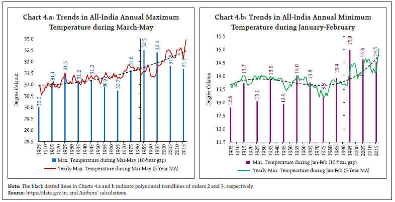 Furthermore, the onset and withdrawal dates of the SWM (since 2010) provide useful information to analyse visible changes in its timeline (Table 1). As per the IMD, the normal dates for the onset and withdrawal of SWM are June 1 and September 1, respectively. The onset of SWM was delayed in five years since 2010 with the average delay being five days. During 2019, the onset was delayed by seven days. What was particularly disruptive was the delay of 39 days in its withdrawal, which is in sharp contrast to the previous nine years.3 The number of days taken by the SWM for its complete withdrawal (eight days only) was also unusual. Additionally, the withdrawal of SWM in 2019 coincided with the onset of the north-east monsoon, a fairly new phenomenon. 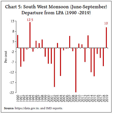
| Table 1: South West Monsoon Onset and Withdrawal Timeline (Number of Days) | | Year | Delay in Onset | Delay in Withdrawal | Time Taken for Complete Withdrawal | | 2010 | 1 | 27 | 33 | | 2011 | 3 | 23 | 32 | | 2012 | -4 | 24 | 25 | | 2013 | 0 | 9 | 43 | | 2014 | -5 | 23 | 26 | | 2015 | -4 | 4 | 46 | | 2016 | -7 | 15 | 44 | | 2017 | 2 | 27 | 15 | | 2018 | 3 | 29 | 23 | | 2019 | -7 | 39 | 8 | | Source: Monsoon reports, IMD. |
Extreme Weather Events Along with gradual changes in temperature and rainfall patterns, extreme weather events, such as excessive/unseasonal rainfall (often leading to floods), severe temperature fluctuations (e.g., heat waves and cold waves) and high wind speeds (e.g., cyclones) are being witnessed with rising frequency and intensity all over the world. In India too, during the past two decades, floods followed by cyclones, unseasonal rainfall and heat waves have been the major types of extreme weather events (Chart 7.a). The frequency of these events has also increased since 2008 (Chart 7.b). Incidents of major floods and torrential rains have been reported largely since 2004, while unseasonal rainfall has been a rising concern since 2011. Moreover, if we look at the regional spread of these events, it is found that some of the major agricultural States (either food grain or cash crop producers) are the most affected (Andhra Pradesh, Odisha, West Bengal, Gujarat, Maharashtra and Madhya Pradesh) (Chart 8). III. Literature Review The literature on climate change and its impact on the economy is overwhelming in terms of both the depth of analysis and coverage of the range of complex issues. While in the context of developed economies a lot of work has been done, the literature is still at a nascent stage for the developing economies. Policy makers and central bankers are also realising the growing economic consequences/risks of climate change, necessitating changes in the systems for modelling and forecasting of macroeconomic variables (Nordhaus, 2017; Batten, 2018). The literature suggests that climate-related disclosures could lead to an orderly transition to a low carbon economy if the process helps a majority of the investors in better evaluation of their financial risk exposures (Batten et al., 2016). With regard to the impact of weather fluctuations on the overall economic health, studies have generally focused on aggregate economic output and agricultural yields. For example, findings from a study show that higher temperatures may not only have an adverse impact on the level of aggregate economic output but may also reduce its growth rate (Dell et al., 2012; Acevedo et al., 2018). Another study shows that during 1964-2007, drought and extreme heat damaged agricultural production significantly across the globe, and recent droughts caused a larger impact on cereals production than the earlier ones (Lesk et al., 2016). Studies also indicate that climate change is causing negative impact on living standards, livestock productivity, and food security in drylands (Mani et al., 2018; IPCC, 2019). Temperature-related extreme weather events have a stronger association with agricultural yield anomalies than precipitation-related factors; irrigation facilities help mitigate the negative effects of temperature extremes but only partially (Vogel et al., 2019). Using a panel dataset of 174 countries for the period 1960-2014, a study finds that per capita real output growth is adversely affected by persistent deviations in temperature from its historical norm (Kahn et al., 2019). It also provides evidence for a sustained negative impact of climate change on real output, labour productivity and employment across many States and sectors. Similar findings for the US are also found in Colacito et al., (2018). Using a Macro Weather Index, a study done in Japan found that a rise in precipitation would result in a decline in consumer spending and a rise in temperature would cause the private consumption to increase in summer and decrease in winter (Akutsu and Koike, 2019). 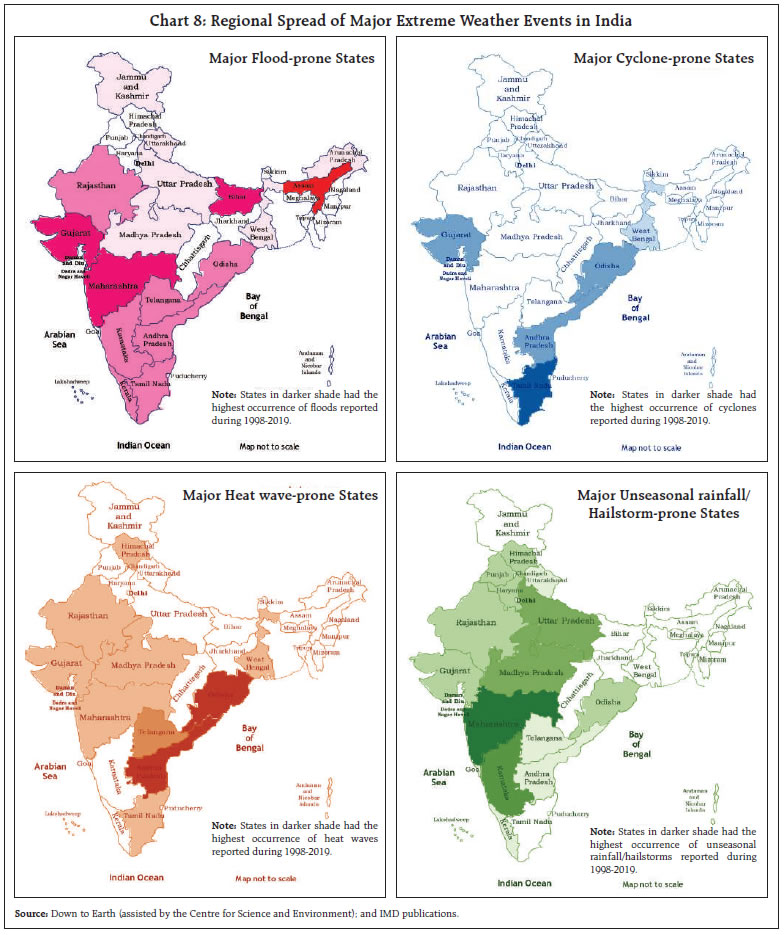 In the Indian context, there are a few studies that have highlighted the risks from climate change primarily on the farm sector (in particular, crop yields) and living standards of people. India is seen to be more vulnerable to climate change than the US, China, Russia, and most other parts of the world, barring Africa (Joshi and Patel, 2009). Using a district-level panel dataset for 1957-2000, it is estimated that a one standard deviation increase in high temperature days in a year decreases agricultural yields and real wages by 12.6 per cent and 9.8 per cent, respectively, while increasing the annual mortality among rural population by 7.3 per cent (Burgess et al., 2014). Another study analysing the impact of exposure to extreme temperatures on crop yields across crops (such as paddy, jowar, ragi and pigeon pea) in Karnataka finds an inverse linear relationship between crop yields and extreme temperature days, with the impact of temperature on yields exceeding that of rainfall (Murari et al., 2018). Furthermore, an increase in temperature is seen to reduce agricultural productivity, while rainfall (unless in excess) tends to nullify it (Birthal et al., 2014). A persistent increase in temperature in India in the absence of risk mitigating policies can cause the per capita GDP to reduce by 6.4 per cent by 2100 (Kahn et al., 2019). IV. Empirical Analysis for India The amount of CO2 emission in India has been a major concern as scientists have argued that the emissions are the main culprit for the rising temperature levels. Also, it is widely believed that increased economic activity results in more emission of CO2. Therefore, to begin with, three sets of pair-wise Granger-causality tests are conducted using data on GDP per capita, CO2 emission (metric tons) per capita, and annual average temperature for the period 1960-2014 in the Indian context. The results show that economic activity measured by GDP per capita causes CO2 emissions and CO2 emissions cause increase in average temperature (Annex Table 2.a). Moreover, the results indicate the existence of a bi-directional causality between temperature and GDP per capita. As expected, rainfall affects the amount of available irrigated area (gross irrigated area), which in turn affects agricultural yield (output and/or sown area) (Annex Table 2.b). The results are also summarised in the form of flowcharts (Illustration 2). Considering the diverse climatic conditions in India at any given point of time, simple averages of weather indicators across all States may not be able to fully capture the true nature of changing patterns. In order to account for this problem, weather indices – temperature index and precipitation index – are computed as weighted averages of deviations from long-run averages. Further, as most of the economic data are available for the economy as a whole and on a monthly frequency, the indices are calculated on a monthly basis at the all India level. Following Bloesch and Gourio (2015), the steps involved in the construction of the indices are outlined below: Step 1: Data on monthly deviations (difference between the monthly average and long-run normal) of temperature and rainfall for the important weather stations of the country are obtained. Let the deviations be denoted as Di, where i represents the State/station. Step 3: The normalised deviations over all States are aggregated by weighting the States by their population (wi), assuming that the economic activity is correlated with population.
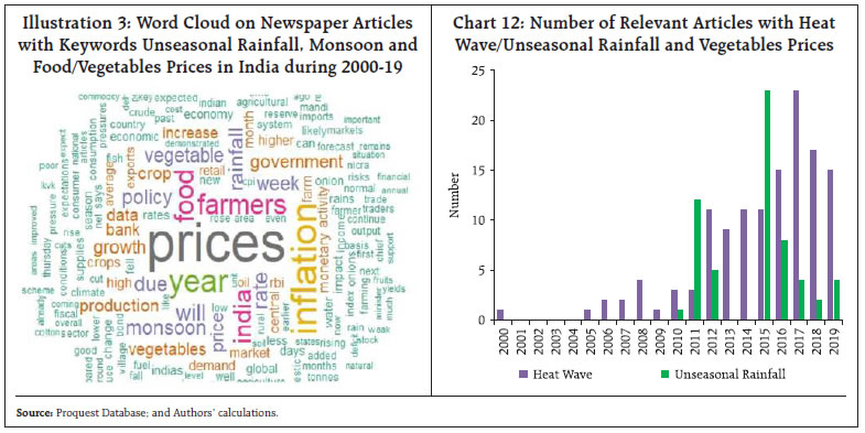
As expected in the Indian context, the scatter plot of the temperature index against the precipitation index constructed for the period October 2009-July 2019 displays a negative and statistically significant correlation [(-)0.32]. This indicates that temperature decreases with an increase in precipitation (Chart 9). Additionally, the correlograms for the precipitation and temperature indices show how long the deviations persist (Chart 10). In the case of temperature index, the correlation falls quickly. The lasting positive correlation in the precipitation index indicates longer monsoons and shrinkage of the gap between the SWM withdrawal and arrival of the north-east monsoon. The impact of climate change on inflation and economic activity are analysed in the next two sub-sections. Here, although there are other factors like sea level and wind patterns that indicate the changing climatic pattern, the analysis is done to study the effect of temperature and precipitation (as measured using the indices) alone for ease.4 IV.1. Impact on Inflation Globally, periods of food price spikes have always been driven by weather-related events with the channel of impact being crop loss/lower agricultural production. During the last six decades, there were three major episodes of significantly high food prices globally: 1970s; 2007-08; and 2010-14, all of which were triggered by adverse weather shocks followed by other factors like increase in oil prices, trade policy interventions and biofuel consumption (Chart 11). 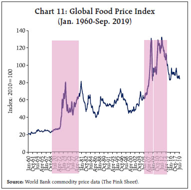 In the case of India, headline inflation5 has moderated significantly over the years alongside a remarkable fall in food inflation (Annex Table 3). With food group comprising 46 per cent of the overall Consumer Price Index (CPI), it remains a crucial determinant of the headline inflation trajectory. Both inflation and its volatility across different food components exhibit distinct patterns. Vegetables inflation has remained high (6.8 per cent) during January 2012-September 2019 along with significantly high volatility (15.8 per cent). Further, it is one of the key components in CPI-food (weight: 13.2 per cent in CPI-Food) having a strong positive correlation with overall food inflation (Table 2). Rainfall deviation has a good association with vegetables inflation and thereby, with overall food inflation. There is growing evidence of newspaper articles covering reports on food prices (especially prices of vegetables) being impacted by unseasonal rainfall and heat waves (Illustration 3 and Chart 12). | Table 2: CPI-Food and Beverages and its Major Components: Summary Statistics | | Components | Correlation with Food Inflation | Average Inflation
(per cent) | Inflation Volatility
(per cent) | | Cereals and products (21.1) | 0.77*** | 5.3 | 4.3 | | Meat and fish (7.9) | 0.81*** | 7.3 | 3.6 | | Egg (0.9) | 0.72*** | 5.9 | 5.4 | | Milk and products (14.4) | 0.64*** | 6.4 | 3.9 | | Oils and fats (7.8) | 0.47*** | 4.6 | 4.7 | | Fruits (6.3) | 0.51*** | 5.9 | 5.5 | | Vegetables (13.2) | 0.78*** | 6.8 | 15.8 | | Pulses and products (5.2) | 0.37*** | 5.2 | 16.5 | | Sugar and confectionery (3.0) | 0.17 | 3.0 | 9.8 | | Spices (5.5) | 0.24** | 4.7 | 4.0 | | Non-alcoholic beverages (2.7) | 0.84*** | 4.9 | 2.4 | | Prepared meals, snacks, sweets etc. (12.1) | 0.82*** | 7.5 | 3.3 | | Food and beverages | 1.00 | 5.8 | 4.3 | ***,** and * represent 1 per cent, 5 per cent and 10 per cent levels of significance, respectively.
Note: 1. Figures in parentheses indicate weight in CPI-Food and beverages.
2. Inflation volatility has been measured using standard deviation.
Source: NSO; and Authors’ calculations. |
 Against this backdrop, we first look at plots of food inflation and vegetables inflation with all India precipitation index (Charts13.a and 13.b). While food inflation reveals some association, the co-movement of vegetables inflation with precipitation index appears stronger. Contemporaneous correlation between the precipitation index and food inflation and its various components show vegetables inflation having the highest correlation of 0.38 with the precipitation index (Table 3)6. Additionally, 12-months rolling correlation coefficients (starting from January 2012) depict periods when correlation between vegetables (food) inflation and precipitation index peaked at 0.70 (Chart 14). 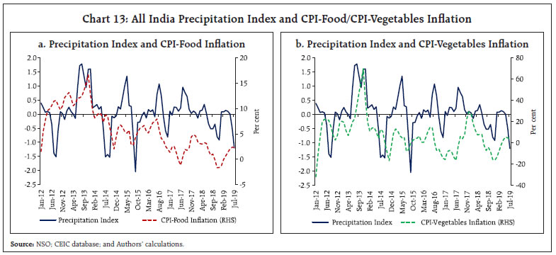
| Table 3: Correlation between Food Inflation, its Components and Precipitation Index | | Components | Correlation Coefficient | P-value | | Cereals and products | 0.26 | 0.01*** | | Meat and fish | 0.18 | 0.08* | | Egg | 0.10 | 0.37 | | Milk and products | 0.02 | 0.82 | | Oils and fats | -0.18 | 0.08 | | Fruits | -0.04 | 0.67 | | Vegetables | 0.38 | 0.00*** | | Pulses and products | -0.11 | 0.29 | | Sugar and confectionery | 0.03 | 0.77 | | Spices | 0.11 | 0.30 | | Non-alcoholic beverages | 0.21 | 0.05** | | Prepared meals, snacks, sweets etc. | 0.16 | 0.13 | | Food and beverages | 0.25 | 0.02** | ***,** and * represent 1 per cent, 5 per cent and 10 per cent levels of significance, respectively.
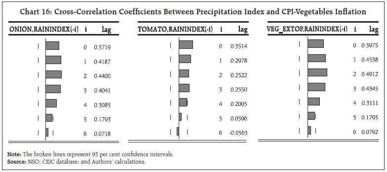
Source: NSO; CEIC database; and Authors’ calculations. | Furthermore, we look at the cross-correlation coefficients, which would capture not only the contemporaneous correlation but would also show the impact of rainfall with lag(s). This is because, in some food components, the impact of rainfall could appear with some time lag, while for others the impact of rain could last for some months. The results reveal that the impact of rainfall usually lasts for 5-6 months in the case of vegetables inflation as well as overall food inflation (Chart 15). Further, for vegetables, the extent of impact could increase with some lag. This is usually the case because vegetables are perishable in nature and the impact on prices is gradually reflected after crops are damaged and adverse supply shocks from the production centres spread across regions. For cereals, we do not find much of a lagged relationship between precipitation index and inflation, which could be primarily on account of cereals being non-perishables and the stabilising role of available buffer stocks/well-defined supply management system in place. Any contemporaneous correlation could be primarily driven by market sentiments amongst traders related to adverse rainfall pattern and crop sowing. For fruits, the precipitation index influences inflation with some lag, which could be because most of the fruits are seasonal and are not produced throughout the year. Therefore, if production is adversely impacted by unfavourable rainfall, the impact on prices is gradual and once affected, could last for a brief period. 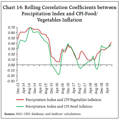 Since prices of vegetables are the most affected by rainfall disturbances, we look at the impact of precipitation index on vegetables prices at a disaggregated level. Within CPI-vegetables, tomato (weight: 9.5 per cent), onion (weight: 10.7 per cent) and potato (weight: 16.3 per cent) together constitute 36 per cent of the total share and the price movements of these three primary vegetables significantly determine overall vegetables inflation. Again, results based on cross-correlation analysis show precipitation index to have a strong and statistically significant impact on inflation in onions, tomatoes and vegetables excluding tomatoes, onions and potatoes (TOP), with the impact continuing for 4-5 months (Chart 16). Potato inflation did not have any statistically significant association with the precipitation index.7 This could be due to the storable nature of potatoes and availability of storage facilities. Price pressures in vegetables, especially onions and tomatoes, were a major concern in 2019-20 owing to significant crop losses and supply disruptions on account of delayed monsoon withdrawal in October, and excessive/unseasonal post-monsoon rainfall leading to floods in major producing States like Maharashtra, Karnataka, Telangana, Madhya Pradesh and Himachal Pradesh. In the past too (specifically, during 2011, 2015, 2017 and 2018), there were episodes of unseasonal rainfall affecting vegetables prices, especially of onions and tomatoes (RBI, 2011; 2015; 2018). 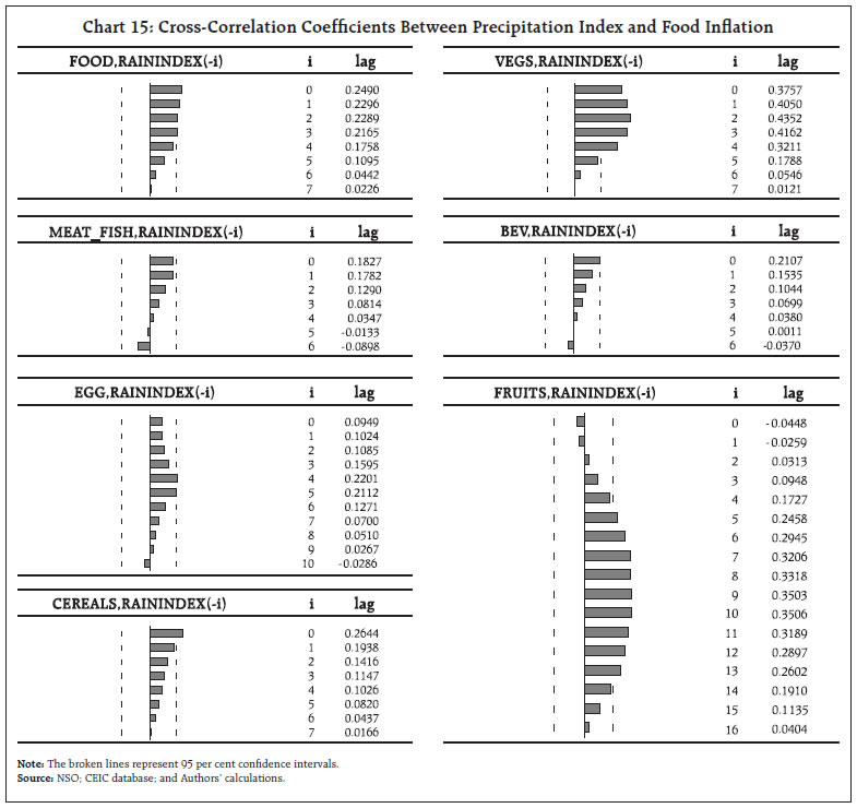
 IV.2. Impact on Economic Activity In order to study the impact of climate change on economic activity, eight high-frequency economic indicators (the data for which are available on a monthly basis) have been used. The indicators have been selected in such a way that they track different sectors of the economy. These indicators include: Foreign Tourist Arrivals, Automobile Sales, Tractor Sales, Demand for Electricity, India’s Total Trade, Purchasing Managers Index (PMI), Index of Industrial Production (IIP) and IIP-Manufacturing Food Products. For the analysis, all variables are seasonally adjusted. Separate time-series regressions for each indicator are performed against the two weather indices as per the following equation: where, Yt, represents one of the eight economic indicators considered at time t, Pt is the precipitation index at time t,Tt, is the temperature index at time t and ɛt is the residual. The results show that rainfall has a larger impact on the economy in comparison to the changes in temperature (Table 4). The negative signs for PMI in the case of both precipitation and temperature indices indicate that as the country gets warmer or when more than expected rains are received, the manufacturing and the service sectors tend to decelerate. The negative impact is observable for total trade as well. Further, as expected, increase in temperature causes the demand for electricity to increase as the requirement for air-conditioners, coolers and refrigerators tend to rise. Tractor sales are positively impacted by the rainfall received. Also, an increase in rainfall tends to accelerate automobile sales. | Table 4: Regression Results9 | | Dependent Variable | Precipitation | Temperature | R-squared | | Foreign Tourist Arrivals10 | 0.007 | 0.002 | 0.016 | | | (0.205) | (0.441) | | | Automobile Sales | 0.015** | 0.002 | 0.043 | | | (0.026) | (0.624) | | | Tractor Sales | 0.020* | 0.007 | 0.030 | | | (0.086) | (0.234) | | | Electricity Power: Demand | 0.005 | 0.005*** | 0.061 | | | (0.192) | (0.009) | | | Total Trade | -0.068** | -0.045*** | 0.068 | | | (0.048) | (0.012) | | | PMI | -0.019*** | -0.005** | 0.222 | | | (0.0000) | (0.049) | | | IIP | 0.002 | 0.001 | 0.011 | | | (0.441) | (0.429) | | | IIP: Mfg. Food Products11 | -0.007 | -0.005 | 0.026 | | | (0.267) | (0.199) | | ***,** and * represent 1 per cent, 5 per cent and 10 per cent levels of significance, respectively.
Note: Figures in parentheses denote p-values. | V. Mitigation of Climate Change Risks Krogstrup and Oman (2019) provide a comprehensive review of the literature on the macroeconomic and financial policies that could be effective in mitigating climate change risks. They conclude that the fiscal tools are the first best options, but should be complemented by appropriate monetary policy instruments. V.1. Fiscal Policy Tools In April 2016, India officially signed the 2015 Paris climate agreement along with other 194 countries. As per the agreement, the increase in global average temperature should be held well below 2 degree Celsius above pre-industrial levels and efforts should be made to limit the temperature increase to 1.5 degree Celsius. According to Krogstrup and Oman (2019), fiscal policy tools can be classified into: (1) price policies (carbon taxation which will force firms and individuals to reduce emissions; and subsidies for mitigation actions); (2) spending and investment (outright public investments and concessional loans); and (3) public guarantees. The IMF’s Fiscal Monitor (October 2019) discusses the use of other instruments in addition to the carbon taxation, which include Emission Trading Systems12, Feebates13 and regulations for setting emission rate standards, or minimum requirements for the use of renewables in power generation. However, creation of awareness is the first step, which would be the prime responsibility of the governing bodies. V.2. Commodity Derivatives Market Currently, the Multi Commodity Exchange (MCX) is the largest commodity futures exchange in India, followed by National Commodity and Derivatives Exchange (NCDEX). The commodities traded include metal, bullion, energy, spices, plantation, pulses, cereals, petrochemicals, oil and oil seeds. Data reveal that futures trading in agricultural commodities is low and the share in total trade has declined in the recent past (Chart 17). Moreover, there has been a sharp decline in the volume of futures/options traded at NCDEX, which is the largest farm futures exchange (Chart 18). Considering the impact of climate change on the economy, a developed commodity derivatives market can help mitigate risks by enabling continuous price discovery and providing a strategy for hedging price risk in the face of uncertainty. Weather derivatives may be viewed as ‘financial instruments whose value and/or cash flows depend on the occurrence of weather related events, which can be identified and measured easily and can serve as underlyings of financial contracts’ (Barrieu and Scaillet, 2009; Considine, 2000). Weather derivatives which were introduced in the US and Europe in 1997 and 1998, respectively have become increasingly popular. The markets have grown tremendously in the US and Europe and have expanded to the over the counter (OTC) markets. The Chicago Mercantile Exchange (CME) has introduced weather derivatives that can be traded electronically on the CME’s GLOBEX platform. The popular contracts are the month futures (swap) contracts based on heating degree days (HDD), which measure how much heating is required in winter; and cooling degree days (CDD), which measure how much cooling is necessary in summer months, along with options on futures (Schlenker and Taylor, 2019). 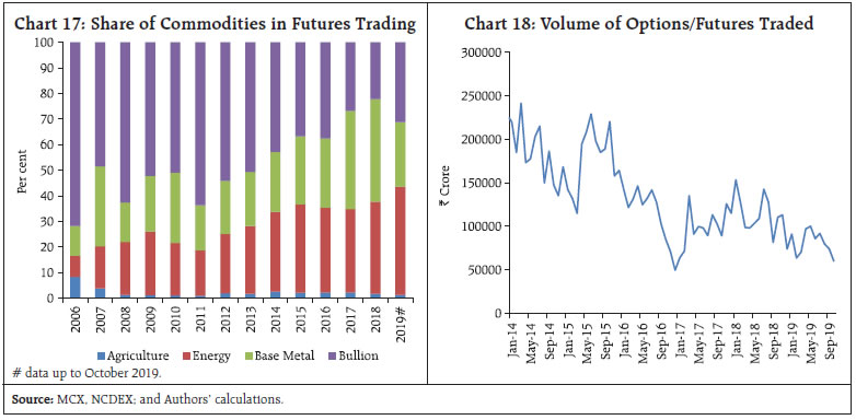 Insurance is normally used to cover the loss due to the occurrence of low-probability, high-risk events. But in the case of weather derivatives, the underlying event need not be necessarily catastrophic and are best suited for high-probability, low-risk events. Considering the climate change patterns witnessed in the country, introduction and popularisation of weather derivatives have become the need of the hour. The challenges in introducing weather derivatives include design issues, choice of appropriate pricing rules, and choice of underlying assets. A pilot run using an appropriate index for rainfall may be conducted in order to explore its significance and feasibility in mitigating risks from unseasonal rainfalls. V.3. Central Banking Tools Central banks would require to monitor two types of risks: physical risks and transition risks (Batten et al., 2016). While physical risks would include damage of balance sheets of households, corporates, banks and insurers triggered by a weather-related event causing financial and macroeconomic instability, transition risks would include the after-effects of the implementation of fiscal policy tools, which could lead to re-pricing of carbon-intensive assets and also trigger negative supply shocks. As per the Central Bank’s Survey on Climate Change for 2019, 64 per cent respondents described climate change as a significant concern. Eight central banks and supervisors established the Central Banks and Supervisors Network for Greening the Financial System (NGFS) in 2017, which is concerned with the analysis and management of risks in the financial sector14. The NGFS provides six recommendations (for central banks, supervisors, policymakers and financial institutions) including integration of climate-related factors into prudential supervision and emphasises the importance of a robust and internationally consistent climate and environmental disclosure framework [NGFS (2019)]. A quick review of suggestions offered by Krogstrup and Oman (2019), Batten et al., (2016), Silva (2019) and the Central Banking Focus Report would indicate the important measures that can be examined by central banks for adoption to mitigate risks from climate change: -
Provide support to activities/initiatives targeting green finance (like the NGFS). -
Include climate risks in the analytical models used in policy formulation and research and perform scenario analysis and stress testing to understand areas where actions would be required. -
Bridge gaps on data related to various environmental aspects of finance. -
As a part of its reserve management, central banks can invest in green assets rather than in brown assets like carbon-intensive assets. -
Provide additional/subsidised liquidity support to banks that invest in environment-friendly products. -
Incentivise banks towards green projects by redesigning capital and collateral rules. -
Encourage regulated/supervised entities (banks) to allocate at least a certain minimum credit to environment-friendly sectors. VI. Conclusion Climatic conditions, comprising the two key indicators - precipitation and temperature, play a crucial role in the overall health of the Indian economy. Over the years, India has witnessed changes in climatic patterns in line with the rest of the world. With increase in population and economic activity, the cumulative level of GHG emissions has increased causing the average temperature to rise over time. Importantly, the rainfall pattern, particularly with respect to the SWM, which provides around 75 per cent of the annual rainfall, has undergone significant changes. Moreover, the occurrence of extreme weather events like floods/unseasonal rainfall, heat waves and cyclones has increased during the past two decades and data reveal that some of the key agricultural States in India have been the most affected by such events. Two separate indices were constructed at the all-India level – the temperature index and the precipitation index – and their impact on food inflation and economic activity indicators was analysed. The results indicated weather conditions, especially rainfall, to have a strong influence on the food inflation trajectory and the impact was found to last for a couple of months. Within food, vegetables prices are the most vulnerable to rainfall shocks. The results also showed weather conditions to have a significant impact on some of the key indicators of economic activity like PMI, IIP, demand for electricity, trade, tourist arrivals, and tractor and automobile sales. This article also highlighted various policy tools that could help mitigate climate change risks. References Acevedo, S., Mrkaic, M., Novta, N., Pugacheva, E., & Topalova, P. (2018), “The Effects of Weather Shocks on Economic Activity: What are the Channels of Impact?”, IMF Working Paper, WP/18/144s. Akutsu, K., and Y. Koike (2019), “Analysis of Private Consumption using Weather Data”, Bank of Japan Review, 2019-E-1. Barrieu, P., and O. Scaillet (2009), “A Primer on Weather Derivatives”, Uncertainty and Environmental Decision Making, 155-175. Batten, S. (2018), “Climate Change and the Macro-Economy: A Critical Review”, Staff Working Paper No. 706, Bank of England. Batten, S., R. Sowerbutts and M. Tanaka (2016), “Let’s Talk About the Weather: The Impact of Climate Change on Central Banks”, Staff Working Paper No. 603, Bank of England. Birthal, P.S., et al., (2014), “How Sensitive is Indian Agriculture to Climate Change?”, Indian Journal of Agricultural Economics, 69 (4), National Centre for Agricultural Economics and Policy Research, New Delhi. Bloesch, J., and F. Gourio (2015), “The Effect of Winter Weather on U.S. Economic Activity”, Federal Reserve Bank of Chicago Economic Perspectives, 39, Number 1. Burgess, R., et al., (2014), “The Unequal Effects of Weather and Climate Change: Evidence from Mortality in India”, available at: https://pdfs.semanticscholar.org/8958/18edb2300f50ffe45417f3c065c722dd1ba4.pdf Central Banking (2019), “Central Banking Focus Report-Climate Change”, in association with Amundi Asset Management. Colacito, R., et al., (2018), “The Impact of Higher Temperatures on Economic Growth”, Economic Brief, Federal Reserve Bank of Richmond. Considine, G. (2000), “Introduction to Weather Derivatives”, available at http://www.agroinsurance.com/files/weather%20derivatives.pdf Dell, M., B.F. Jones and B.A. Olken (2012), “Temperature Shocks and Economic Growth: Evidence from the Last Half Century”, American Economic Journal: Macroeconomics, 4 (3), 66-95. IMF (2019), “Fiscal Monitor-How to Mitigate Climate Change”, October, Washington DC, USA. IMF (2019), “Global Financial Stability Report”, October, Washington DC, USA. IMF (2019), “World Economic Outlook”, April, Washington DC, USA. IMF (2019), “World Economic Outlook”, October, Washington DC, USA. Indian Environment Portal: http://www.indiaenvironmentportal.org.in IPCC (2018), “Global Warming of 1.5°C”, Special Report, Switzerland. IPCC (2019), “Climate Change and Land”, Summary for Policymakers, Approved Draft. Joshi, V., and U. R. Patel (2009), “India and Climate Change Mitigation”, Smith School Working Paper Series, Working Paper 003, Smith School of Enterprise and the Environment, University of Oxford, UK. Kahn, M.E., et al., (2019), “Long-term Macroeconomic Effects of Climate Change: A Cross-Country Analysis”, NBER Working Paper Series, Working Paper 26167. Krogstrup, S., W. Oman, (2019), “Macroeconomic and Financial Policies for Climate Change Mitigation: A Review of the Literature”, IMF Working Paper, No. 19/185. Lesk, C., P. Rowhani and N. Ramankutty (2016), “Influence of Extreme Weather Disasters on Global Crop Production”, Nature, 529, 84-99. Mani, M., et al., (2018), “South Asia’s Hotspots: The Impact of Temperature and Precipitation Changes on Living Standards”, World Bank Group, Washington DC, USA. Murari, K., et al., (2018), “Extreme Temperatures and crop Yields in Karnataka, India”, Review of Agrarian Studies, 8 (2). NGFS (2019), “A call for action-Climate change as a source of financial risk”, available at https://www.banque-france.fr/sites/default/files/media/2019/04/17/ngfs_first_comprehensive_report_-_17042019_0.pdf Nordhaus, W.D. (2017), “Projections and Uncertainties about Climate Change in an Era of Minimal Climate Policies”, NBER Working Paper Series, Working Paper 22933. RBI (2011), “Reserve Bank of India Annual Report 2010-11”, Mumbai. RBI (2015), “Reserve Bank of India Annual Report 2014-15”, Mumbai. RBI (2018), “Reserve Bank of India Annual Report 2017-18”, Mumbai. Rudebusch, G.D. (2019), “Climate Change and the Federal Reserve”, FRBSF Economic Letter. Schlenker, W., and C. A. Taylor (2019), “Market Expectations about Climate Change”, NBER Working Paper Series, Working Paper 25554. Silva, L A P da (2019), “Research on Climate-related Risks and Financial Stability: An Epistemological Break?”, Conference of the Central Banks and Supervisors Network for Greening the Financial System (NGFS), Paris, April. United Nations https://www.un.org/en/sections/issues-depth/climate-change/ United Nations Framework Convention on Climate Change https://unfccc.int/ Vogel, E., et al., (2019), “The Effects of Climate Extremes on Global Agricultural Yields”, Environmental Research Letters, 14.
| Annex Table 1: Climate Change and Macroeconomy – Transmission Channels and Risks | | Type of shock/impact | Physical Risks | Transition Risks | | From extreme weather events | From gradual global warming | | Demand | Investment | Uncertainty about climate events | | ‘Crowding out’ from climate policies | | Consumption | Increased risk of flooding to residential property | | ‘Crowding out’from climate policies | | Trade | Disruption to import / export flows due to natural disasters | | Distortions from asymmetric climate policies | | Labour supply | Loss of hours worked due to natural disasters | Loss of hours worked due to extreme heat | | | Energy, food and other inputs | Food and other input shortages | | Risks to energy supply | | Supply | Capital stock | Damage due to extreme weather | Diversion of resources from productive investment to adaptation capital | Diversion of resources from productive investment to mitigation activities | | Technology | Diversion of resources from innovation to reconstruction and replacement | Diversion of resources from innovation to adaptation capital | Uncertainty about the rate of innovation and adoption of clean energy technologies | | Source: Batten (2018). |
| Annex Table 2.a: Pairwise Granger Causality Tests | | Null Hypothesis | P-value | | GDP per capita does not Granger Cause CO2 Emissions per capita | 0.008 | | CO2 Emissions per capita does not Granger Cause GDP per capita | 0.392 | | Temperature does not Granger Cause CO2 Emissions per capita | 0.983 | | CO2 Emissions per capita does not Granger Cause Temperature | 0.000 | | Temperature does not Granger Cause GDP per capita | 0.085 | | GDP per capita does not Granger Cause Temperature | 0.000 |
| Annex Table 2.b: Pairwise Granger Causality Tests | | Null Hypothesis | P-value | | Agriculture yield does not Granger Cause Rainfall | 0.162 | | Rainfall does not Granger Cause Agriculture yield | 0.000 | | Gross Irrigated Area does not Granger Cause Rainfall | 0.168 | | Rainfall does not Granger Cause Gross Irrigated Area | 0.000 | | Gross Irrigated Area does not Granger Cause Agriculture yield | 0.001 | | Agriculture yield does not Granger Cause Gross Irrigated Area | 0.481 |
| Annex Table 3: CPI Headline Inflation and Its Major Components | | Components | 2012-13 | 2013-14 | 2014-15 | 2015-16 | 2016-17 | 2017-18 | 2018-19 | 2019-20
(Apr.-Sep.) | | Food and beverages (45.86) | 11.2 | 11.9 | 6.5 | 5.1 | 4.4 | 2.2 | 0.7 | 2.6 | | Fuel and light (6.84) | 9.7 | 7.7 | 4.2 | 5.3 | 3.3 | 6.2 | 5.7 | 0.5 | | Excluding food and fuel (47.30) | 9.0 | 7.2 | 5.4 | 4.6 | 4.8 | 4.6 | 5.8 | 3.3 | | All Groups | 10.0 | 9.4 | 5.8 | 4.9 | 4.5 | 3.6 | 3.4 | 4.3 | Note: Figures in parentheses indicate weight in CPI-Combined.
Source: NSO; and Authors’ calculations. |
| Annex Table 4: Results of the Unit Root Tests | | Variables | Augmented Dickey Fuller Test Statistic | Phillips-Perron Test Statistic | | X | ΔX | X | ΔX | | Foreign Tourist Arrivals | -0.182 | -9.727*** | -0.387 | -29.786*** | | Automobile Sales | -1.910 | -13.367*** | -2.287 | -14.592*** | | Tractor Sales | -3.016 | -9.311*** | -2.660 | -16.058*** | | Electricity Power: Demand | -0.325 | -15.339*** | -0.323 | -17.275*** | | Total Trade | -2.093 | -22.254*** | -1.957 | -19.867*** | | IIP | 0.333 | -10.567*** | 0.480 | -25.973*** | | IIP: Mfg. Food Products | -0.089 | -10.629*** | -0.162 | -25.561*** | | PMI | -4.695*** | - | -4.640*** | - | ***,** and * represent 1 per cent, 5 per cent and 10 per cent levels of significance, respectively.
Source: NSO; and Authors’ calculations. |
|