Executive Summary Global growth remained resilient in 2026 so far, supported by AI-related investment, and fiscal stimulus measures, despite disruptions due to the ongoing West Asia conflict. Renewed energy-price pressures stoked inflation pressures and prompted a more hawkish stance from leading central bank. Fiscal sustainability concerns, persistent inflation, and geopolitical uncertainty raised bond yields, while equity markets remained volatile amid lingering concern on valuations technology stocks. Amidst global uncertainty, domestic financial markets underwent intermittent volatility during H1:2026-27. System liquidity surplus surged in September 2026, mainly on account of the Reserve Bank’s swap facilities. Overnight rates in the money market evolved in sync with prevailing liquidity conditions. Transmission to lending and deposit rates plateaued with status quo in policy rate during H1:2026-27. Bank credit growth became broad based and strengthened further. The domestic economy showed resilience in H1:2026-27, despite continued global uncertainty amidst the conflict. The supply-side pressures were alleviated by proactive policy measures by the government that ensured adequate supply of key inputs. Real GDP recorded a growth of 7.8 per cent in Q1:2026-27 reflecting strong momentum in underlying economic activity. Aggregate demand remained strong on the back of both private consumption and investment. Net external demand was also robust and contributed significantly to growth. On the supply side, both manufacturing and services sectors recorded strong growth in Q1. High frequency indicators suggest continued buoyancy in domestic economic activity, albeit with some moderation compared to Q1. Stable employment conditions, congenial financial conditions, revival in corporate investment, and a pickup in goods exports – nurtured by bilateral FTAs and diversification – are expected to support economic activity going forward. Sustenance of private consumption growth will be essential for broad-based recovery in private capex. Headline CPI inflation increased sequentially, rising above the target during June-August, driven by a sustained positive price momentum. Food and fuel groups led to this increase, reflecting adverse weather conditions and the sharp rise in energy prices following the West Asia conflict. Core inflation registered a pick-up with some signs of generalisation in recent months. Input cost pressures have accentuated, but the pass-through has remained limited so far. Going forward, India’s macroeconomic outlook remains resilient supported by domestic demand and strengthening investment, despite persistent global uncertainties. The outlook remains vulnerable to geopolitical developments, volatility in global energy markets and weather-related uncertainties. Weak monsoons coupled with strong El Niño, protracted geopolitical tensions, rising international commodity prices, additional frictions in global trade and tightening of global financial conditions could adversely impact the growth outlook. Persistent supply-side pressures in food and volatile global energy prices pose risks to the domestic inflation outlook, particularly through second-round effects amid strong growth impulses. The interplay of these factors will shape the evolving growth–inflation dynamics, with the balance of risks depending on developments in global growth, crude oil prices, exchange-rate movements, and domestic food supplies.
I. External Environment Global growth remains resilient, mainly supported by AI-related investment and fiscal measures, but faces renewed supply-side shocks from the West Asia conflict, elevated oil prices and trade related frictions. Inflation has accelerated again, prompting central banks to shift towards a more cautious and hawkish monetary policy stance. Financial markets remain volatile amid higher yields, geopolitical tensions and shifting risk sentiment. Global growth has remained resilient despite facing persistent headwinds from supply shocks. However, the near-term growth forecasts have been revised downwards by several multilateral agencies, as key supply chains remain disrupted and crude oil prices remain elevated. Investment in artificial intelligence (AI) and related technologies, along with increased international trade in AI-related hardware, has supported global economic activity. Fiscal support across countries has sustained economic activity but also heightened concerns about rising public debt and reduced fiscal buffers. Along with higher inflation and higher-for-longer monetary policy expectations, these concerns have contributed to a sharp rise in government bond yields across major jurisdictions. Inflation, which had been moderating towards the end of 2025, began to accelerate following the supply shock triggered by the West Asia conflict. Crude oil prices rose to levels not seen in recent years. At the same time, other commodity prices also increased, feeding into higher goods inflation even as services inflation remained elevated in several major economies. Consequently, central banks that had been moving towards monetary policy normalisation last year adopted a more hawkish stance following the onset of the conflict. Several advanced and emerging market economies (EMEs) have tightened monetary policy or maintained a cautious stance, while only a handful have reduced policy rates to support growth. Of late, the US Fed and the European Central Bank (ECB) have been placing greater emphasis on incoming data and their monetary policy frameworks in decision making, rather than on forward guidance. The Fed’s hawkish stance, combined with elevated crude oil prices, contributed to risk-off sentiment and portfolio outflows from EMEs, exerting depreciation pressure on their currencies. Sovereign bond yields have hardened globally, particularly in advanced economies (AEs), on concerns over rising public debt, debt-servicing costs and persistent inflation concerns. Emerging market equities experienced selloffs during Q3 of 2026, with some recovery in August while advanced economy equities gained, driven by technology stocks and healthy corporate profits. The US dollar gained, as higher bond yields, expectations of a hawkish Fed, and safe-haven demand amid geopolitical uncertainty outweighed intermittent weakness. I.1 Global Economic Conditions In 2026 so far, global growth has remained resilient, even as near-term growth forecasts have been revised downwards amid the fragile geopolitical situation in West Asia. The growth outlook is dependent on the de-escalation of the conflict, as key supply chains continue to face disruptions, and oil prices remain elevated. In its July 2026 World Economic Outlook update, the International Monetary Fund (IMF) lowered its global growth projection for 2026 by 10 bps to 3.0 per cent, reflecting the uncertainty around the outlook. However, it raised its projection by 20 bps for 2027 to 3.4 per cent, as the impact of the conflict remains less than what was anticipated earlier, while AI-related investment and productivity gains are likely to fuel growth. Meanwhile, the OECD, in its September 2026 Interim Economic Outlook, marginally raised its global growth forecast by 10 bps to 2.9 per cent for 2026, while lowering its 2027 projection by 10 bps to 3.0 per cent. While AI-related activity is expected to provide continued support, stronger price pressures and elevated interest rates are likely to weigh on near-term growth momentum. Among AEs, real GDP growth in the US remained resilient in 2026, supported by robust consumer spending and investment, including continued private investment in AI and related technologies. Growth, however, moderated in the second quarter, reflecting a downturn in government spending, slower investment and export growth, while stronger consumer spending partly offset these effects (Table I.1). Since April 2026, labour market conditions have softened, with non-farm payroll growth slowing down during summer and weakening further in September, while the unemployment rate remained largely stable. The composite PMI continued to expand strongly in August, recording a 52-month high, driven by services while manufacturing remained healthy amid improved business optimism and new orders. Consumer sentiment, as measured by the University of Michigan Survey, declined in September to its lowest level in four months, amid growing concerns about elevated prices. Overall, underlying economic activity in the US remains resilient. Among other AEs, growth in Japan in 2026 so far has been largely driven by the external sector. GDP growth strengthened in Q1, with net exports making the largest contribution. Growth moderated in Q2 due to slowdown in domestic demand, particularly private investment, though this moderation was offset largely by a strong contribution from net exports. The composite PMI continued to expand in August, driven by manufacturing while services also improved. On the other hand, GDP growth recovered in the euro area in Q2 after stagnating in Q1, primarily driven by strong growth in Ireland and Spain. Household and government expenditure continued to provide support to economic activity. The composite PMI expanded in August at the same pace for the second consecutive month as the moderation in services was offset by solid expansion in manufacturing amid growth in new orders and factory output. In the UK, GDP growth rebounded in Q1 2026, supported by services and broad-based expansion across the economy, with gross capital formation and household consumption driving growth on the expenditure side. Growth moderated in Q2, reflecting weaker household consumption and lower inventory accumulation amid the adverse effects of the conflict in West Asia. Among high-frequency indicators, the composite PMI expanded in August for the second consecutive month, driven by services sector activity offsetting the moderation in manufacturing. | Table I.1: Real GDP Growth | | (Per cent) | | Country | Q3-2025 | Q4-2025 | Q1-2026 | Q2-2026 | 2025 | 2026 (P) | 2027 (P) | | Quarter-on-quarter, seasonally adjusted, annualised rate (q-o-q, saar) | | Canada | 1.9 | -1.0 | 0.3 | 3.3 | 1.9 | 1.1 | 1.7 | | Euro area | 1.3 | 0.9 | 0.0 | 2.6 | 1.4 | 0.9 | 1.2 | | Japan | -1.5 | 1.1 | 1.9 | 1.4 | 1.1 | 0.6 | 0.7 | | South Korea | 5.6 | -0.4 | 7.5 | 2.6 | 1.1 | 2.6 | 2.5 | | UK | 0.7 | 0.0 | 2.6 | 2.1 | 1.4 | 1.0 | 1.3 | | US | 3.9 | 0.2 | 2.5 | 2.2 | 2.1 | 2.3 | 2.2 | | Year-on-year | | Brazil | 1.8 | 1.8 | 1.8 | 2.0 | 2.3 | 2.4 | 2.2 | | China | 4.8 | 4.5 | 5.0 | 4.3 | 5.0 | 4.6 | 4.1 | | India | 8.1 | 7.7 | 8.6 | 7.8 | 7.7 | 6.4 | 6.7 | | Indonesia | 5.0 | 5.4 | 5.6 | 5.3 | 5.1 | 5.0 | 5.1 | | Philippines | 4.0 | 3.0 | 2.8 | 2.3 | 4.4 | 3.9 | 5.5 | | Russia | 0.8 | 1.0 | -0.2 | 1.3 | 1.0 | 1.1 | 1.1 | | South Africa | 2.1 | 0.8 | 1.9 | 0.9 | 1.1 | 1.1 | 1.3 | | Thailand | 1.2 | 2.5 | 2.8 | 1.9 | 2.4 | 1.9 | 2.2 | | Memo: | | World | 2025 | 2026 (P) | 2027 (P) | | Year-on-year | | Output | 3.5 | 3.0 | 3.4 | | Trade volume | 5.0 | 3.5 | 4.3 | P: Projection.
Notes: 1. India's data correspond to fiscal year (April-March); e.g., 2026 pertains to April 2026-March 2027.
2. Projectons for 2026 and 2027 are taken from the IMF WEO, July 2026 update.
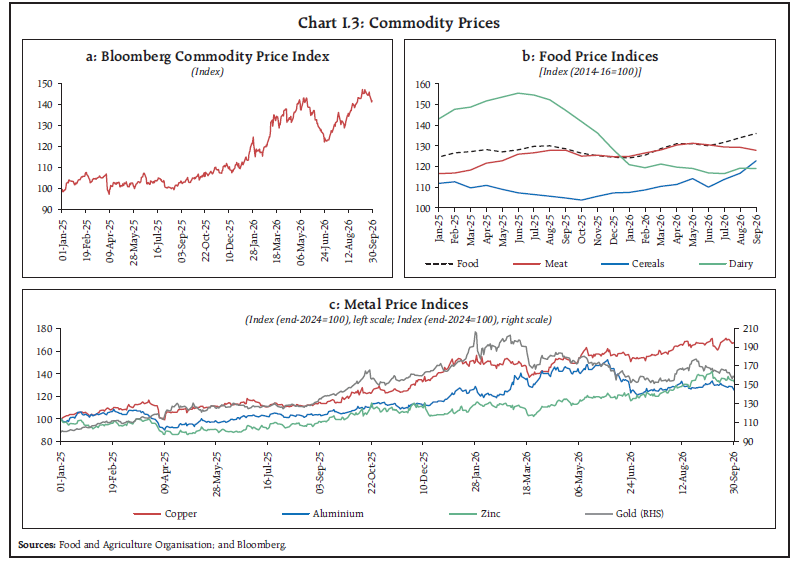
Sources: Official statistical agencies; Bloomberg; and IMF. | Among major EMEs, China’s growth is facing challenges from subdued consumption and a weaker external sector in 2026, with GDP growth moderating in Q2 from Q1. The composition of growth has also undergone a shift, with the share of net exports in GDP growth declining significantly relative to 2025, while the share of gross capital formation increased. Investment growth remains uneven, with stronger activity concentrated in AI-related and high-tech sectors. High-frequency indicators also point to subdued activity, with composite PMI slowing in July as both manufacturing and services sector activity moderated. In August, however, PMI rebounded as output and new orders increased in both the sectors but remained below the average for 2026. Brazil’s GDP growth remained stable at 1.8 per cent (y-o-y) in Q1, marking the third consecutive quarter of growth at this pace. The agriculture and services sectors supported growth while industrial activity declined. In Q2, however, GDP expanded by 2.0 per cent, driven by recovery in industrial sector and sustained growth in agriculture. Industrial sector benefited from higher oil and gas extraction amid higher energy prices. Brazil’s composite PMI remained very close to the neutral line in the last few months, reflecting weakness in the economy as new orders continue to fall. Russia’s economy contracted in Q1, reflecting weak manufacturing and construction activity, although services remained resilient. Activity recovered in Q2, led by manufacturing, while agriculture remained subdued. The composite PMI also returned to expansion in August, ending five consecutive months of contraction, supported by stronger output and new orders. In South Africa, GDP growth accelerated in Q1, driven by a recovery in agriculture, increased mining activity, and stronger momentum in services, before moderating in Q2 led by a contraction in manufacturing and mining. Composite PMI continued to remain around neutral line in August amidst subdued new orders and weak business confidence. The Asian Development Bank (ADB), in its September 2026 outlook, projected ASEAN1 growth at 4.7 per cent in both 2026 and 2027. The outlook remains subject to downside risks from the West Asia conflict, elevated energy and commodity prices, weaker external demand and heightened global uncertainty. Turning to high-frequency indicators, the OECD’s composite leading indicators (CLIs) showed that most economies remained above their long-term trend in Q2 and Q3 (till August) of 2026 (Chart I.1a). The global composite PMI expanded at its quickest pace in August in more than two years, with broad-based expansion in both output and new orders (Chart I.1b). The services sector continued to expand in August for the fifth straight month, while the manufacturing sector remained solid. 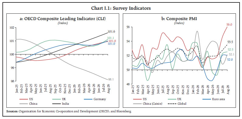 World merchandise trade expanded for eleven consecutive quarters through Q2:2026, with growth remaining robust and exceeding expectations. Both EMEs and AEs contributed to the expansion, though the impulse came largely from EMEs, with moderation in contribution by the AEs as frontloading of US imports moderated. In July 2026, world merchandise trade volume growth remained strong at 6.0 per cent (y-o-y), with EMEs contributing 3.2 percentage points and AEs 2.8 percentage points (Chart I.2a). The surge in trade of electronic components related to AI offset the negative impact of the conflict in West Asia. The WTO, in its March 2026 update, revised its projection for global merchandise trade volume growth from 0.5 per cent to 1.9 per cent in 2026, reflecting strong AI-related trade and a smaller-than-anticipated impact of tariffs. The Goods Trade Barometer (September 2026, WTO) remained above trend at 102.0, with the electronic components and other goods linked to investment in artificial intelligence (AI) indices indicating continued momentum in merchandise trade. Meanwhile, shipping costs remained elevated, with the Freightos Baltic Global Index staying higher in 2026 - above its 2025 average - reflecting the rerouting of vessels away from disrupted shipping corridors/chokepoints and continued capacity pressures (Chart I.2b). I.2 Commodity Prices and Inflation Commodity prices, as captured by the Bloomberg Commodity Index, have exhibited divergent movements, largely attributable to sector-specific fundamentals (Chart I.3a). Agricultural commodity prices have risen due to conflict-related disruptions to energy, fertiliser and shipping markets, adverse weather conditions and tighter crop-supply prospects. Global food prices, as reflected in the Food and Agriculture Organisation (FAO) food price index, have increased since April 2026, mainly due to vegetable oils, cereals, and sugar (Chart I.3b). Gold prices declined through Q2 2026 amid expectations of higher interest rates. Gold prices gained overall in Q3 as heightened geopolitical uncertainty, including renewed tensions in West Asia, boosted safe-haven demand. Periods of weakness in the US dollar and lower expectations of further tightening by the Fed also supported prices, outweighing the drag from rising bond yields and the stronger dollar in September. Among base metals, copper and zinc prices have continued to rise, supported by tightening supply conditions. Aluminium prices rose to a four-year high in early June amid concerns over supply disruptions from the West Asia conflict, before moderating as the US dollar strengthened and Chinese exports increased (Chart I.3c). 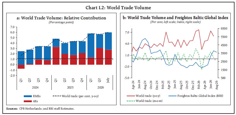
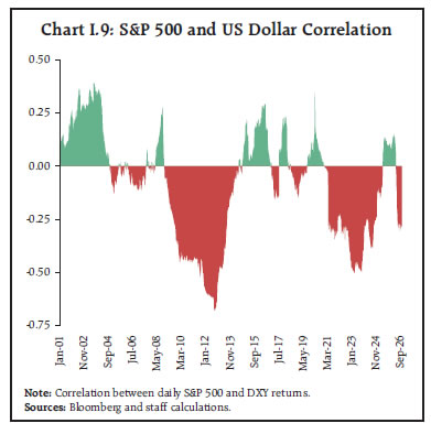
 Energy prices surged in April, largely reflecting the sharp increase in Brent prices, before moderating as supply disruptions eased. However, the re-escalation of tensions in West Asia led to a renewed increase in energy prices in August and September, amid concerns over disruptions in regional oil production and shipping (Chart I.4a). Against this backdrop, developments in global oil supply buffers and demand conditions remain important. The US Strategic Petroleum Reserve (SPR) is currently placed at roughly 284 million barrels, at its lowest level since October 1982. Strategic releases and inventory drawdowns helped to cushion shocks. Also, weaker import demand by China due to release of stocks and domestic demand destruction helped offset some supply pressures. However, if the disruptions last longer, there is lower flexibility available to deal with supply shortages (Chart I.4 b&c). Consumer Price Inflation Inflationary pressures have re-emerged following a temporary moderation, driven primarily by renewed energy and commodity price pressures amid heightened West Asia tensions. 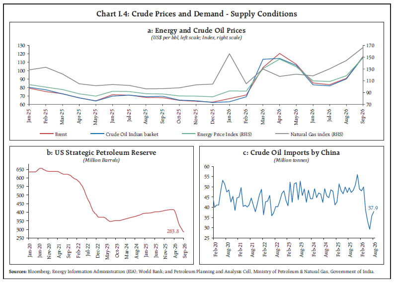 The US personal consumption expenditures (PCE) price index, the Federal Reserve’s preferred inflation metric, saw inflation surge through May, driven by a sharp increase in gasoline prices before falling subsequently as energy prices stabilised. In the UK, headline inflation has been lower in Q2 2026, mainly due to easing food inflation, before edging up in Q3 so far on rising energy and housing prices. In the euro area, energy prices and persistently high service inflation drove the CPI inflation higher, except for a modest correction in June due to a reversal in crude prices. In Japan, inflation rose steadily from April, reflecting a slower decline in energy prices as subsidies were scaled back in Q2, alongside imported inflation from yen depreciation. Inflation rose further in Q3, on elevated food prices and transportation costs, despite lower electricity prices. In EMEs, inflation has been divergent, reflecting differences in domestic demand conditions and supply-side pressures across economies. In Brazil, the headline CPI rose due to food and beverages, then fell as food, transport, and housing prices moderated. Inflation in South Africa accelerated from April to June, driven predominantly by higher fuel and transport costs, before easing in July as fuel prices declined and food-price inflation moderated. In Russia, CPI inflation eased until May on easing food pressures before edging higher due to fuel and a weaker rouble. China’s CPI inflation has remained subdued, supported by persistent food-price deflation (Chart I.5b). I.3 Monetary Policy Stance Since April 2026, monetary policy actions have diverged across economies. However, major advanced economy central banks turned more hawkish in Q3 2026, as renewed West Asia tensions raised energy prices and intensified inflationary pressures. Among major AEs, the US Fed held the target range at 3.50–3.75 per cent through July. In September, amidst persistent inflationary pressures, robust economic activity and stable labour-market conditions, the Fed unanimously raised the target range by 25 basis points to 3.75–4.00 per cent. The Bank of England has maintained the policy rate unchanged at 3.75 per cent in the last six meetings, noting little evidence so far of material second-round effects from the energy shocks while reiterating that future policy decisions depend on how the energy shock evolves and its impact on inflation. 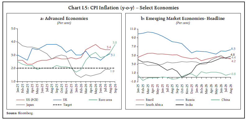 The ECB raised its key policy rates by 25 basis points in June and again in September, taking the deposit facility rate to 2.50 per cent. The decisions reflected persistent energy-driven inflation pressures associated with the conflict; however, indirect and second-round effects have remained largely contained. The Bank of Japan (BoJ) continued policy normalisation, raising its policy rate by 25 basis points each in June and September to 1.25 per cent. The moves reflected persistent inflationary pressures, owing to higher import costs amid yen depreciation, with future policy decisions to be guided by developments in economic activity and prices. The Reserve Bank of Australia raised rates in May amid elevated inflation and capacity pressures, and again in September as fuel-price pass-through and stronger-than-expected growth intensified inflation risks. The Bank of Canada maintained status quo as longer-term inflation expectations have remained anchored and there was little evidence that oil prices had fed through more broadly to goods and services prices. The Reserve Bank of New Zealand hiked the policy rate by 25 bps for the first time in three years in July and then again in September by the same magnitude to 2.75 per cent. The monetary policy committee considered gradual withdrawal of monetary stimulus as appropriate to steer inflation to the 2 per cent target, while supporting growth and employment (Chart I.6a). Among key EMEs, Brazil continued its monetary easing cycle, with the central bank reducing the Selic rate in successive meetings amid signs of moderating economic activity and easing inflationary pressures. The Bank of Russia has gradually reduced its key rate as economic growth edged lower. China has held its benchmark rate at 3.0 per cent for more than a year amid ample liquidity. South Africa raised its policy rate by 25 basis points to 7.25 per cent in September, following a similar increase in May, amid rising inflation risks and concerns over potential second-round effects. The Bank of Thailand kept its policy rate unchanged, balancing weaker growth and subdued domestic demand against conflict-related, supply-driven inflation pressures. The Bank of Mexico cut its policy rate by 25 basis points to 6.5 per cent in May, marking the end of its easing cycle. In September, it kept rates unchanged but removed its earlier forward guidance, signalling greater policy flexibility (Chart I.6b). 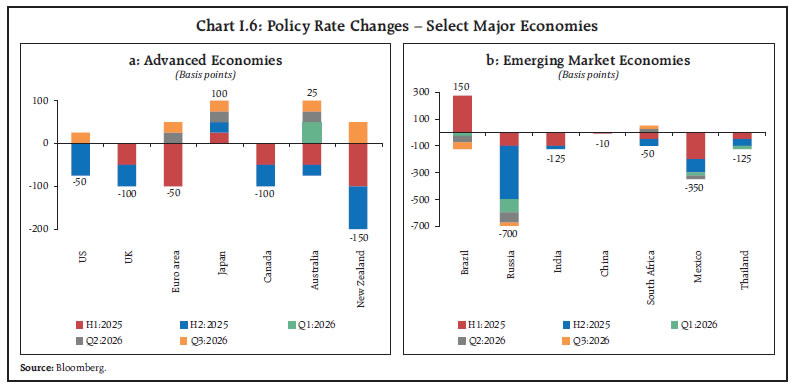 I.4 Financial Markets Global financial markets remained largely resilient yet volatile, guided by the interplay of AI-driven risk appetite, shifting monetary policy expectations, elevated sovereign borrowing needs, and persistent geopolitical tensions in West Asia. The stock-bond correlation in the AEs has shifted for the first time in decades, reflecting uncertainty due to supply-side shocks (Box I.1). Box I.1: Stock–Bond Correlation in Advanced and Emerging Economies The equity–government bond return correlation is central to multi-asset portfolio diversification. Stock–bond return correlation is influenced by short-term rates, inflation, volatility, and economic growth (Aslanidis and Christiansen, 2012). Theoretical explanations link asset-price co-movement to macroeconomic conditions (Campbell et al., 2020), while changes in stock–bond correlation have important implications for portfolio diversification (Brixton et al., 2023). More recently, evidence from G7 economies suggests that the macroeconomic drivers of stock–bond correlation vary over time, with significant implications for portfolio risk and diversification (McMillan, 2026). After two decades of generally positive readings, the correlation in advanced economies turned sharply negative during the 2021–22 inflation surge and again in 2025 (Chart I.1a). Using a DCC-GARCH model, the analysis finds that stock–bond correlation in advanced economies follows an inflation-regime relationship. Inflation enters with a negative linear and positive quadratic term, implying that correlation is lowest near the inflation target and rises as inflation moves away from it (Chart I.1b). The implied turning point is 1.6 per cent, essentially at the 2 per cent target, and the real short rate is also positive and significant. The findings suggest that when inflation is moderate, government bonds tend to hedge equity-market risk. 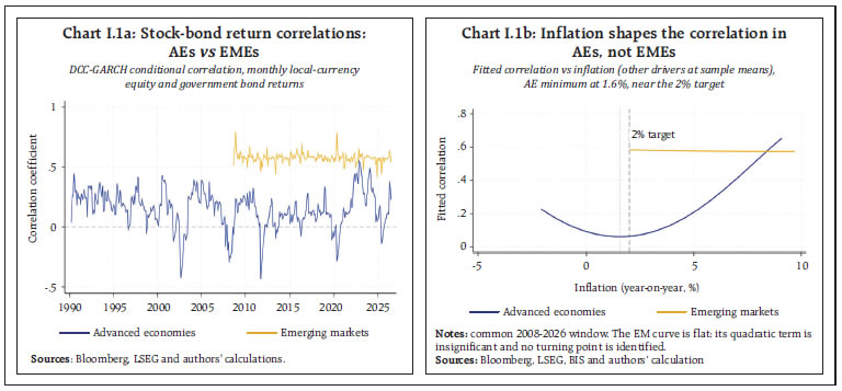 This mechanism, however, does not extend to emerging markets. Their correlation averages around +0.6 and never turns negative over the sample, while its relationship with domestic inflation is weak and statistically insignificant. A formal Wald test also rejects equality of the advanced- and emerging-market coefficients. Instead, global equity volatility (VIX) is the only significant explanatory variable. The results suggest that emerging-market government bonds behave more like risk assets than domestic safe havens, selling off alongside equities when global risk appetite deteriorates. Thus, their diversification benefits are not evident in the post-2008 sample, unlike in advanced economies. References: 1. Aslanidis, N., & Christiansen, C. “Smooth Transition Patterns in the Realized Stock–Bond Correlation”. Journal of Empirical Finance, 19(4), 454–464, 2012. 2. Brixton, A., Brooks, J., Hecht, P., Ilmanen, A., Maloney, T., & McQuinn, N. “A Changing Stock–Bond Correlation: Drivers and Implications”. The Journal of Portfolio Management, 49(4), 64–80, 2023. 3. Campbell, J. Y., Pflueger, C., & Viceira, L. M. “Macroeconomic Drivers of Bond and Equity Risks”. Journal of Political Economy, 128(8), 3148–3185, 2020. 4. McMillan, D. G. “Stock-Bond Return Correlation: Understanding the Changing Behaviour”. Journal of International Financial Markets, Institutions and Money, 106, Article 102242, 2026. | Global equities advanced in Q2 2026, driven by continued momentum in artificial intelligence (AI) and related capital investment cycles (Chart I.7a). Geopolitical tensions in West Asia added sporadic volatility during the quarter. The announcement of a US–Iran ceasefire framework and a memorandum of understanding (MoU) eased concerns about a broader regional conflict. Energy prices recoiled, and investor sentiment improved as fears of a sustained disruption to global energy supplies diminished. During Q2, US equities advanced, supported by resilient corporate earnings and sustained investor enthusiasm for AI-related companies. In the euro area, equities posted solid gains, with IT outperforming amid strong corporate earnings and diversification by investors from US markets. In the UK, equity prices rose, although declines in energy stocks limited overall gains. Markets largely looked through domestic political developments, with investor sentiment remaining broadly resilient. Japanese equities delivered robust returns in Q2 as easing tensions in West Asia buoyed sentiment, while the yen – at a four-decade low against the US dollar – supported exporters. In Q3, major equity markets posted modest gains, although investor sentiment remained cautious amid expectations of further monetary tightening, elevated technology-sector valuations, and persisting tensions in West Asia. Equities gained in the US, supported by resilient corporate earnings and sustained AI optimism, with further support from the Fed’s commitment to combating inflation despite its hawkish stance. Euro-area equities declined in Q3 as higher energy prices and persistent inflation lifted bond yields and weighed on risk sentiment, while political uncertainty and fiscal concerns, added to investor caution. Japanese equities were affected by the global correction in AI-related stocks and also concerns surrounding a stronger yen which could weigh on exports. In the UK, equities made modest gains, supported by robust corporate earnings, and elevated commodity prices. Equity markets in most EMEs rose sharply in Q2:2026, outperforming global peers. Taiwan and Korea led market performance, driven by gains in memory and semiconductor stocks amid strong AI demand (Chart I.7b). In Q3, emerging-market equities surrendered the gains recorded in the previous quarter as the AI-led rally showed signs of fatigue. Renewed conflict in West Asia, heightened trade tensions, and expectations of a more hawkish Fed weighed on investor risk appetite. 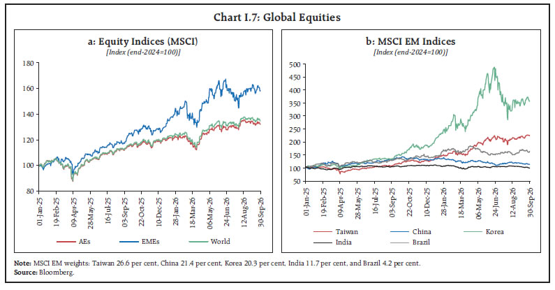 A global sell-off in government debt led by inflation persistence and high government deficits has raised borrowing costs. These pressures have been exacerbated by the West Asia conflict, which has driven up oil prices, leading investors to seek higher bond yields as the odds of rate cuts have largely diminished. Sovereign bond-market performance diverged in Q2: Japanese and US rates firmed up, while German and UK yields softened. Developments in West Asia continued to be a major driver of the market, with bond yields moving in tandem with oil prices. Yields on government bonds surged to multi-year highs around the middle of the quarter amid fears of further escalation but fell on signs of a possible US–Iran deal. In the US, rates were underpinned by a resilient labour market and elevated government debt, reinforcing expectations that monetary policy would remain tight. A combination of global inflation concerns, and domestic politics hit UK gilts. In April, the 10-year gilt yield hit its highest level since 2008, reflecting inflationary pressures from higher oil prices and concerns about budgetary and political vulnerabilities ahead of municipal elections. Higher oil costs and imported-inflation pressures from the yen supported expectations for BoJ policy hikes this year, while concerns about fiscal expansion contributed to upside pressure. In Q3, government bond yields in major AEs have risen amid persistent energy-price pressures and tighter monetary policy, while elevated public debt and renewed fiscal support have added to upward pressure on long-term yields. In the US, higher oil prices, persistent inflation concerns, and higher borrowing requirements pushed treasury yields higher. The Treasury’s decision in mid-August to expand buybacks of long-dated securities provided only temporary relief, as underlying inflation and term-premium pressures continued to weigh on the market. Elsewhere, government bond yields in the euro area, Japan and the UK moved up amid renewed inflation concerns from rising energy prices, while rate hikes and firm policy signals, along with country-specific fiscal risks and elevated sovereign borrowing requirements, added to the rise in yields (Chart I.8 a). Emerging-market 10-year sovereign bonds recorded a mixed performance, displaying divergent country-specific inflation, fiscal, and monetary policy dynamics. While favourable risk sentiment and easing expectations initially supported some markets, the subsequent rise in oil prices, US sovereign bond yields, and geopolitical tensions tightened external financing conditions, increasing borrowing costs and weighing more heavily on sovereigns vulnerable to fiscal and external risks (Chart I.8b). In currency markets, the US dollar strengthened in Q2 2026, supported by higher oil prices, heightened geopolitical tensions and still elevated inflation, which reinforced safe-haven demand and expectations of relatively tighter monetary policy. Most major currencies weakened against the US dollar, with the yen declining to a four-decade low despite large scale coordinated intervention by the US and the Bank of Japan. The euro also depreciated, while sterling demonstrated greater resilience. In Q3, the US dollar, which had remained broadly weak through much of the quarter, strengthened markedly in September. The rebound was driven by higher US bond yields and a repricing of expectations for further Fed tightening following the release of data suggesting resilient activity and persistent inflation concerns. Renewed geopolitical tensions in West Asia, elevated oil prices, and trade-related uncertainty also supported safe-haven demand for the dollar. Consequently, the dollar index rose by around 2.0 per cent during September to a near two-month high, although it ended Q3 only marginally higher. Against this backdrop, the renewed negative correlation between the S&P 500 and the US dollar since April indicates that the dollar has again provided a partial hedge during periods of equity-market stress, appreciating when risk sentiment deteriorated and weakening as risk appetite recovered (Chart I.9). Shifts in monetary policy expectations, geopolitical developments, and global risk appetite can, however, quickly alter the stock–dollar correlation. 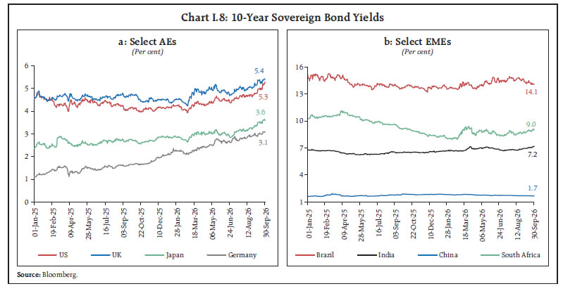
 The MSCI EM Currency Index rose driven by carry-seeking flows, supportive commodity prices and country-specific inflows. However, gains moderated late in the period amid renewed pressure from rising long-term US bond yields (Chart I.10 a & b). I.5 Conclusion The global economic outlook continues to be shaped by supply-side shocks emanating from the West Asia crisis, shifting trade tariffs, and the ongoing AI investment boom. Despite multilateral agencies projecting slower global growth in 2026, high-frequency indicators, including purchasing managers’ indices, point to resilient economic activity. Inflation has picked up in most economies, prompting central banks to adopt a more hawkish stance. Long-term bond yields have risen amid persistent inflation concerns, while equity markets have advanced, underpinned by the ongoing AI-driven investment boom. Elevated inflation, coupled with heightened risks to growth outlook, warrants a cautious approach from the monetary authorities going ahead. _________________________________________________________________________________
II. Liquidity Conditions and Financial Markets System liquidity surplus surged during H1:2026-27 mainly on account of the Reserve Bank’s swap facilities. Overnight rates in the money market evolved in sync with prevailing liquidity conditions. Domestic financial markets exhibited two-way movements amidst global uncertainty. Transmission to lending rates moderated with status quo on policy rate since February 2026. Bank credit growth accelerated further. Sectoral trends indicate broad-based credit expansion. Introduction Global financial markets remained volatile amidst shifting expectations, persistent tensions in West Asia and rising fiscal concerns. Against this backdrop, domestic financial markets displayed intermittent volatility during H1:2026-27. System-wide liquidity surplus surged in September 2026 reflecting buoyant capital flows under the Reserve Bank’s swap facilities. Money market rates largely moved in line with the evolving liquidity conditions, with rates in Certificates of Deposit (CDs) and Commercial Papers (CPs) easing in Q2. The exchange rate exhibited two-way movements in H1. Monetary policy transmission to lending rate moderated during H1 amidst rate pause and funding pressure. Nonetheless, bank credit continued to grow robustly and financing from non-bank sources also increased. II.1 Liquidity Conditions and the Operating Procedure of Monetary Policy The Reserve Bank of India (RBI) Act, 1934 requires the Reserve Bank to place the operating procedure relating to the implementation of monetary policy and changes thereto from time to time, if any, in the public domain.1 During H1:2026-27, the Monetary Policy Committee (MPC) kept the policy rate unchanged in three successive meetings while retaining the neutral policy stance. Drivers and Management of Liquidity System liquidity, as measured by the net balances under the liquidity adjustment facility (LAF), improved significantly in H1:2026–27 from a moderate surplus in H2:2025–26 (Chart II.1). On a net basis, average daily absorption under the LAF increased to ₹3.21 lakh crore in H1:2026–27 from ₹1.43 lakh crore in H2:2025–26. Capital inflows and the build-up of government cash balances were the principal drivers of liquidity conditions in H1:2026–27. System liquidity remained in surplus during H1:2026-27 except for end-June when it briefly turned into deficit amidst tax related outflows.2 In Q1, liquidity conditions improved initially supported by faster government spending, but it moderated thereafter due to increase in currency in circulation (CiC) and the RBI’s foreign exchange operations. Liquidity conditions improved in Q2, aided by capital inflows under the RBI's swap facilities (Table II.1). 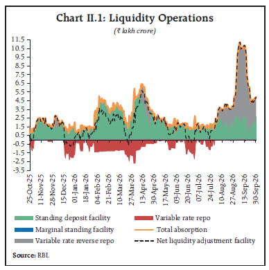 With liquidity conditions remaining largely in surplus, banks’ recourse to the marginal standing facility (MSF) averaged ₹0.01 lakh crore during H1:2026-27, while average daily standing deposit facility (SDF) balances increased marginally3. The Reserve Bank remained nimble and agile in its liquidity management operations, ensuring sufficient liquidity in the banking system to support transmission to money market. With surge in liquidity surplus mainly due to FCNR(B) swaps4, the RBI conducted variable rate reverse repo (VRRR) operations of varying maturities, although several variable rate repo (VRR) operations were also undertaken mainly until July 2026 to tide over transient liquidity tightness and align overnight rates with the policy rate. Overall, the RBI conducted a total of 36 VRR and 51 VRRR auctions in H1. On a review of current and evolving liquidity conditions, the Reserve Bank also conducted OMO sale auctions of Government of India securities for an aggregate amount of ₹1 lakh crore.5 | Table II.1: Liquidity - Key Drivers and Management | | (₹ crore) | | | 2025-26 | 2025-26 | 2026-27 | 2026-27 | 2026-27 | | H1 | H2 | Q1 | Q2* | H1* | | Drivers | | | | | | | (i) CiC [withdrawal (-) /return (+)] | -74,052 | -3,67,073 | -1,29,065 | -8,019 | -1,37,084 | | (ii) Net Forex Purchases (+)/ Sales (-) | -1,41,591 | -3,27,863 | -1,36,182 | 9,12,616 | 7,76,434 | | (iii) GoI Cash Balances [build-up (-) / drawdown (+)] | -3,44,103 | 2,15,110 | -1,80,676 | -25,018 | -2,05,694 | | (iv) Excess Reserves [build-up (-) / drawdown (+)] | 14,376 | -5,849 | -8,646 | 3,345 | -5,301 | | Management | | | | | | | i) Net OMO Purchases (+)/ Sales (-) | 2,39,223 | 6,38,344 | 10 | - | 10 | | (ii) Required Reserves [including both change in NDTL and CRR] | 15,674 | 1,38,046 | -25,807 | -20,920 | -46,727 | | (iii) Term VRR Auctions | 25,731 | 1,36,504 | - | - | - | | (iv) Term VRRR Auctions | - | - | - | 3,19,725 | 3,19,725 | | Memo Items | | | | | | | (i) Long term Forex Swaps Buy/Sell (+)/ Sell/Buy (-)^ | | 2,26,885 | 47,800 | - | 47,800 | | (ii) Net Absorption (+)/ Injection (-) under LAF as at end-period | 56,274 | 3,22,439 | 1,23,964 | 9,88,822 | 9,88,822 | Notes: 1. (+) / (-) sign suggests accretion to / depletion of banking system liquidity.
2. Data pertain to the last reporting day of the respective period.
3. *: Data for Q2 and H1:2026-27 are up to September 15, 2026.
4. ^: approximate values.
5. - : Nil.
Source: RBI. | As on September 15, 2026, reserve money expanded by 8.5 per cent (y-o-y) as against 5.6 per cent a year ago. Adjusted for the first-round impact of CRR change, growth in reserve money stood at 11.9 per cent (9.4 per cent a year ago). The higher growth in reserve money was driven by expansion in currency in circulation. As on September 15, 2026, growth (y-o-y) in money supply (M3) accelerated to 16.6 per cent from 9.2 per cent a year ago owing to faster growth in both aggregate deposits and currency with the public. The money multiplier increased to 6.3 as on September 15, 2026, from 5.8 a year ago, propelled by a declining currency-deposit ratio. II.2 Domestic Financial Markets Money market rates softened in H1:2026-27 in tandem with evolving liquidity conditions. G-sec yields eased until August before hardening in September, reflecting higher global yields, rising oil prices, and expectations of monetary tightening. Corporate bond yields moved in sync with G-sec yields, with a hardening bias, while risk premia showed mixed trends. Equity markets gained marginally despite heightened volatility in global financial markets and crude oil prices due to West Asia conflict. The foreign exchange market remained volatile amid shifting US policies and lingering conflict in West Asia. In the credit market, both bank and non-bank credit grew at a robust pace. II.2.1 Money Market During H1:2026-27, money market rates softened and remained mostly range bound amid large surplus liquidity conditioned by robust capital inflows, especially from FCNR(B) deposits under the Reserve Bank’s swap facility announced in June 2026. The weighted average call rate (WACR) – the operating target of monetary policy – generally remained within the policy rate corridor. However, with the significant rise in surplus liquidity, it moved downward towards the SDF rate, floor of the corridor, in September (Chart II.2a). Volatility in the WACR, as measured by the exponential weighted moving average (EWMA)6, declined considerably in the beginning of FY 2026-27, however, it increased marginally in July, and remained moderate till September (Chart II.2b). Reflecting the evolving liquidity conditions, the average spread of WACR over the policy repo rate turned positive during May-July 2026, before turning negative in August and plunging further in September (Chart II.2b). Overnight rates in the collateralised segment, i.e., triparty repo (TREPS) and market repo, broadly tracked the WACR, although both fell below the SDF rate intermittently during H1:2026-27 (Chart II.3). 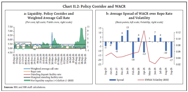 Money market activity remained concentrated in the collateralised segments (tri-party and market repo), with their share in overnight money market volume at 97 per cent. During H1:2026-27, the share of the uncollateralised segment, i.e., the call money market, persisted around 3 per cent. Mutual funds remained the major lenders in tri-party repo with their share unchanged at 65 per cent in H1:2026-27, while their share in total lending in market repo segment moderated to 41 per cent in H1 from 48 per cent in H2:2025-26. The share of foreign banks in market repo lending increased to 31 per cent in H1:2026-27 from 29 per cent in H2:2025-26. On the borrowing side, public sector banks (PSBs) were the major player in tri-party repo, with their share increasing to 35 per cent in H1:2026-27 from 32 per cent in H2:2025-26. The share of private banks reduced noticeably to 14 per cent from 24 per cent. The share of PSBs in market repo increased by 5 percentage points to 13 per cent over the same period. The rates in term segments of the money market also moved in line with the evolving liquidity conditions and uncertainty (also see Box II.1). While 3-month treasury bill (T-Bill) rates moved largely in line with the policy repo rate, the rates on certificates of deposits (CDs) and commercial papers (CPs) edged up in May, but moderated since July notwithstanding intermittent spikes. The average spread of CDs and CPs over the policy repo rate widened to 135 bps and 155 bps in H1:2026-27 from 116 bps and 136 bps, respectively, in H2:2025-26. The average spread of T-Bills over the policy repo rate increased to 5 bps from 1 bp over the same period (Chart II.3). 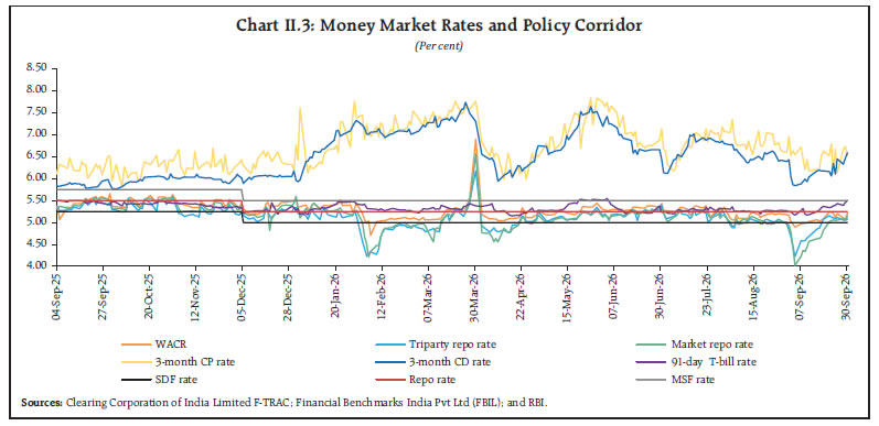
Box II.1: Drivers of CD and CP Rate Spreads Rates on short-term instruments like Certificates of Deposit (CDs) and Commercial Papers (CPs) generally move in tandem with the policy repo rate but diverge at times reflecting broader liquidity conditions and funding pressures. Starting from Q3 of 2025-26, CD/CP rates hardened and remained elevated even as the monetary policy easing cycle continued. It resulted in widening of spread of CD/CP rates over the policy repo rate. Besides liquidity conditions and funding pressures, several other factors can cause CP and CD spreads to deviate from their long-run averages, including, policy uncertainty, monetary policy expectations and market-specific factors such as issuance patterns, calendar effects, and episodes of market stress (Priyadarshini et al., 2024, Anshul et al., 2025). To disentangle the respective contribution of various factors which are intertwined and may operate simultaneously, uncorrelated shocks are identified using historical decompositions within a VAR framework using monthly data. The following VAR specification is used.  Where Yt includes the selected endogenous variables, Xt contains the exogenous dummies and Pεt are the orthogonalised shocks. The variables are selected to capture the main channels, viz., banking system liquidity, funding conditions and policy uncertainty through which they can affect short-term funding costs, while avoiding overlap across closely related measures.7 For CDs, the funding block also captures banks’ balance-sheet pressures through changes in outstanding credit-deposit ratio and net CD issuance growth. For CPs, only net issuance growth is used to capture funding conditions. The uncorrelated shocks are identified using a recursive identification scheme where the most exogenous factors are placed at the top while the response variable, i.e., CD or CP spreads are placed at the end of the ordering. Historical decomposition for the period January 2025 – July 2026 show the extent of contribution by each identified factor to the movements in spreads (Chart II.1.1). 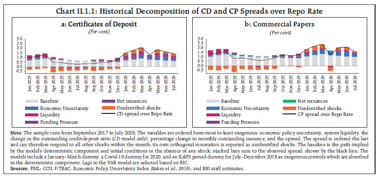 The decomposition results suggest that the drivers of CD and CP spreads have shifted over time. Relatively tight liquidity conditions were the main driver of widening spreads during early 2025, but increased system liquidity along with policy rate easing led spreads to moderate to relatively lower levels by mid-2025. Since late 2025, the spreads hardened again. Funding pressures, owing to stronger credit growth relative to deposit mobilisation, contributed to hardening of CD spread, while economic policy uncertainty was the main driver of widening CP spread. More recently, idiosyncratic market-specific pressures have also contributed to the widening which are unrelated to the identified shocks in the model. References Anshul, Priyadarshini, P. and Chaudhari D. R. (2025), “Drivers of CD Issuances: An Empirical Assessment”. RBI Bulletin. June. Baker, S. R., Bloom, N., & Davis, S. J. (2016), “Measuring Economic Policy Uncertainty”, The Quarterly Journal of Economics, 131(4), 1593-1636. Priyadarshini, P., Anshul, S. S., Chaudhari, D. R., & Das, S. (2024), “Drivers of Commercial Paper Rate Spread-An Empirical Assessment”, RBI Working Paper Series No. 02. | Fresh issuances of CDs reduced considerably in H1:2026-27 compared to H2:2025-26, mainly due to mobilisation of deposits under FCNR(B) scheme and the resulting liquidity surplus (Table II.2). The share of CD issuances of shorter tenor (up to 91-day) decreased while that of longer tenor increased in Q2 compared to Q1 of 2026-27. In contrast to the CD market, CP issuances were robust during H1:2026-27, as rates moderated on the back of large surplus liquidity which incentivised corporates and NBFCs to raise cheaper short-term credit (Chart II.4a; Table II.3). The money market risk premia (spread of 3-month CP rate over 91-day T-bill rate) moderated, tracking the reduction in uncertainty in H1:2026-27 (Chart II.4b).
| Table II.2: Tenor wise Break up of CD Issuances | | (₹ lakh crore) | | | 2025-26 | 2026-27 | | H1 | H2 | Q1 | Q2 | H1 | | Up to 91 Days | 3.55 | 4.40 | 3.00 | 2.15 | 5.14 | | | (73) | (51) | (92) | (81) | (87) | | 92-180 Days | 0.47 | 0.61 | 0.11 | 0.25 | 0.36 | | | (10) | (7) | (3) | (10) | (6) | | 181-365 Days | 0.84 | 3.58 | 0.17 | 0.24 | 0.42 | | | (17) | (42) | (5) | (9) | (7) | | Total | 4.86 | 8.59 | 3.28 | 2.65 | 5.93 | | | (100) | (100) | (100) | (100) | (100) | Notes: 1. Figures in parentheses denote share of each maturity profile.
2. Figures may not add up to total due to rounding off.
Sources: Clearing Corporation of India Limited F-TRAC; and RBI staff estimates. | Corporates dominated CP issuances with their share increasing to 39 per cent in H1:2026-27 from 32 per cent in H2:2025-26 (Chart II.5). In terms of maturity profile, the 91-180 days segment had the largest share (51 per cent) in fresh issuances followed by the 31-90 days segment (Table II.3). II.2.2 Government Securities Market Government securities (G-sec) yields experienced periodic bouts of volatility during H1:2026-27 due to challenging global environment and rise in global bond yields (Chart II.6). In the wake of the West Asia conflict and a sharp rise in crude oil prices, G-sec yields remained elevated during April-May but softened generally in June-July as tensions in West Asia abated temporarily. Yields softened across the term structure during June-July 2026 as FPI debt flows improved after the announcement of special measures, including the expansion of the universe of Fully Accessible Route (FAR) securities by the Reserve Bank and tax concessions by the Government (Chart II.7a). 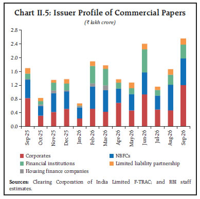
| Table II.3: Maturity Profile of CP Issuances | | (₹ lakh crore) | | Tenor | H1: 2025-26 | H2: 2025-26 | H1: 2026-27 | | 7- 30 days | 0.43 | 0.66 | 1.01 | | | (5) | (8) | (9) | | 31-90 days | 3.10 | 1.87 | 3.80 | | | (35) | (24) | (34) | | 91-180 days | 4.56 | 4.24 | 5.67 | | | (51) | (53) | (51) | | 181-365 days | 0.86 | 1.16 | 0.60 | | | (10) | (15) | (5) | | Total | 8.95 | 7.93 | 11.09 | | | (100) | (100) | (100) | | Outstanding (as at end-period) | 4.89 | 4.60 | 6.22 | Notes: 1. Figures in parentheses denote share of each maturity profile.
2. Figures may not add up to total due to rounding off.
Sources: Clearing Corporation of India Limited F-TRAC; RBI staff estimates. |
After remaining range-bound in early August, the yields hardened again in September, owing to the rise in advanced economy yields, higher domestic inflation print and upward pressure on Brent crude oil prices following renewed West Asia tensions. Overall, the level of yield curve remained elevated during H1 (Chart II.7b). The average trading volume in G-secs increased in H1:2026-27 relative to H2:2025-26 (Chart II.8). The weighted average yield on traded maturities for G-secs rose by 29 bps during the same period. As part of active debt consolidation, the Reserve Bank conducted six switch auctions of G-secs amounting to ₹1.1 lakh crore during H1:2026-27, on behalf of the Government of India. Furthermore, against the backdrop of an improved cash position, the Reserve Bank accepted offers totalling ₹25,704 crore through buyback auctions. The weighted average maturity (WAM) of the outstanding stock of G-secs increased from 13.70 years at end-March 2026 to 13.76 years as at end-September 2026, while its weighted average coupon (WAC) moderated from 7.17 per cent to 7.15 per cent over the same period.
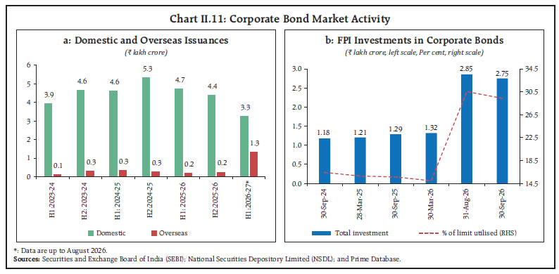
The weighted average spread of cut-off yields on State Government Securities (SGS) over G-sec yields of comparable maturities was 51 bps in H1:2026-27 as against 57 bps in H2:2025-26 (Chart II.9). The average inter-state spread of cut-off yields on SGS of 10-year tenor (fresh issuances) was 6 bps in H1:2026-27 as against 12 bps in H2:2025-26. II.2.3 Corporate Bond Market Corporate bond yields evolved in sync with G-sec yields with a hardening bias during H1:2026-27, while the risk premia showed mixed trends (Chart II.10a). The average bond market risk premium (i.e., the spread of 3-year AAA corporate bond yields over 3-year G-sec yields) hardened from 129 bps to 140 bps for NBFCs, and from 112 bps to 122 bps for corporates, but remained stable at 109 bps for Public Sector Units (PSUs), Financial Institutions (FIs) and banks in H1, even as corporate earnings remained robust in Q1 (Chart II.10b and Table II.4). 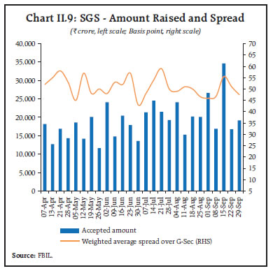 Primary issuances of listed corporate bonds in domestic markets declined by 17.9 per cent during H1:2026-27 (up to August 2026) as compared to the corresponding period of the previous year reflecting higher yields (Chart II.11a). Overseas issuances increased to ₹1,31,931 crore during H1:2026-27 (up to August 2026) from ₹10,303 crore during the same period last year, partly attributed to RBI’s swap facility. Most of the resource mobilisation in the corporate bond market (99 per cent) was through the private placement route. Outstanding investments by foreign portfolio investors (FPIs) in corporate bonds stood at ₹2.7 lakh crore as at end-September, 2026 with utilisation of investment limits at 29.3 per cent (Chart II.11b). Trading volume in the secondary market moderated to ₹9.5 lakh crore during H1 (up to August 2026) from ₹10.1 lakh crore during the corresponding period of the previous year. II.2.4 Equity Market During H1:2026-27, Indian equity markets gained despite heightened volatility in global financial markets and crude oil prices due to conflict in West Asia. Markets rebounded in April 2026 following the announcement of the US-Iran ceasefire. However, equity market remained subdued in May and early June as persistent tensions in West Asia, elevated crude oil prices and the IMD’s forecast of below normal monsoon weighed on investor sentiment. Thereafter, markets gained reflecting resilient corporate earnings results and a rebound in net buying by FPIs, even as the disruption of the US-Iran ceasefire reversed some gains in early July. Equity prices declined towards the end of August and early September amidst lingering geopolitical uncertainties, rising crude oil prices and higher global bond yields. | Table II.4: Financial Markets – Rates and Spread | | | Interest Rates
(Per cent) | Spread (bps)
(Over corresponding risk-free rate) | | Instruments | September 2025 | March 2026 | September 2026 | September 2025 | March 2026 | September 2026 | | 1 | 2 | 3 | 4 | 5 | 6 | 7 | | Corporate Bonds | | | | | | | | (i) AAA (1-yr) | 6.69 | 7.40 | 7.53 | 100 | 171 | 148 | | (ii) AAA (3-yr) | 7.10 | 7.36 | 7.85 | 105 | 112 | 122 | | (iii) AAA (5-yr) | 7.20 | 7.52 | 7.81 | 86 | 92 | 96 | | (iv) AA (3-yr) | 8.20 | 8.22 | 8.63 | 215 | 198 | 200 | | (v) BBB-minus (3-yr) | 11.88 | 11.92 | 12.23 | 583 | 567 | 561 | Note: Yields and spreads are computed as monthly averages.
Source: FIMMDA. |
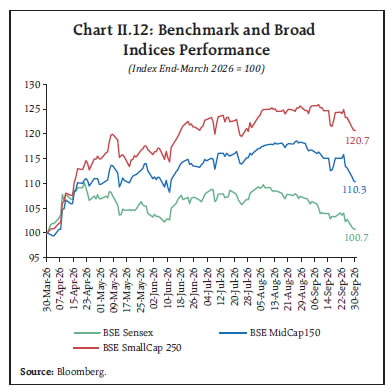 Overall, broader market indices outperformed the benchmark during H1:2026-27 (Chart II.12). However, the price-to-earnings (PE) ratio diverged across market segments. The PE ratio for the benchmark BSE Sensex moderated marginally to 19.2 at end-September 2026 from 19.8 at end-March 2026, while the PE ratio for the MidCap index declined to 29.3 from 31.1 during this period. In contrast, the PE ratio for the SmallCap index rose sharply to 34.6 at end-September 2026 from 26.3 at end-March 2026. The India Volatility Index, a measure of short-term expected volatility of Nifty 50, reduced to 13.5 from 27.9 during this period. Most of the sectors gained in H1. Foreign portfolio investors (FPIs) remained net sellers in H1:2026-27. Domestic institutional investors (DIIs), especially mutual funds, acted as a counterbalancing force with net buying (Chart II.13), which is partly responsible for PE ratios remaining elevated. Resource mobilisation in primary equity markets stood at ₹2.6 lakh crore during H1 (up to August 2026), higher than ₹1.8 lakh crore during the corresponding period a year ago (Chart II.14). II.2.5 Foreign Exchange Market The foreign exchange market remained volatile during H1:2026-27, driven by shifting US policies on tariff and policy rate, and lingering conflict in West Asia. While the rupee initially depreciated in the aftermath of the West Asia conflict, policy measures announced by the Reserve Bank and the Government to bolster capital flows arrested its decline. The implied volatility cooled down after peaking to a multi-year high in the wake of the West Asia conflict (Chart II.15). Overall, the rupee depreciated by 1.4 per cent against the US dollar in H1:2026-27, a marked moderation from the sharp depreciation of 6.2 per cent witnessed in H2:2025-26 (Chart II.16). The relative standing of the rupee among EM currencies also improved even as the pressures from volatile global market, elevated crude oil prices and the prolonged West Asia conflict weighed on the currency. Forward premia moderated during H1:2026-27 from the peak seen in the first week of April, supported by measures undertaken by the Government and the Reserve Bank to attract foreign capital. Upward pressures persisted, however, reflecting volatility in crude oil prices and flare-up of tensions in West Asia conflict (Chart II.17).
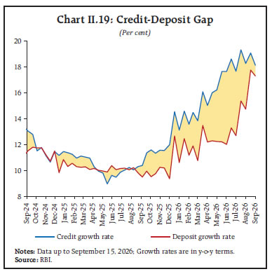
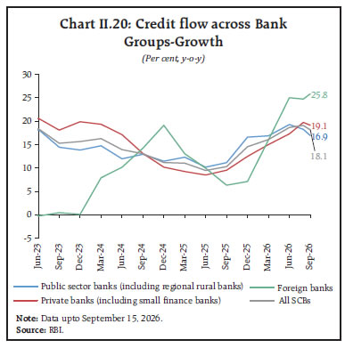
In terms of the 40-currency real effective exchange rate (REER), the INR depreciated by 0.5 per cent between March and August 2026, driven by the depreciation of the rupee in nominal terms (Chart II.18a). During the period, the movement in REER index was modest, as compared to major peer emerging economies (Chart II.18b). II.2.6 Bank and Non-Bank Credit Bank Credit: Aggregate Trends Bank credit growth strengthened further during H1: 2026–27 (up to September 15), on the back of robust loan demand (Chart II.19). As on September 15, 2026, credit growth (y-o-y) for scheduled commercial banks (SCBs) accelerated sharply to 18.1 per cent, from 10.4 per cent during the corresponding period in the previous year (Chart II.20). Across bank groups, foreign banks recorded the highest credit expansion at 25.8 per cent y-o-y, outperforming private banks (PVBs) at 19.1 per cent and public sector banks (PSBs) at 16.9 per cent. While PSBs contributed the largest share to y-o-y incremental credit, their overall market share contracted due to aggressive lending by both PVBs and foreign banks. 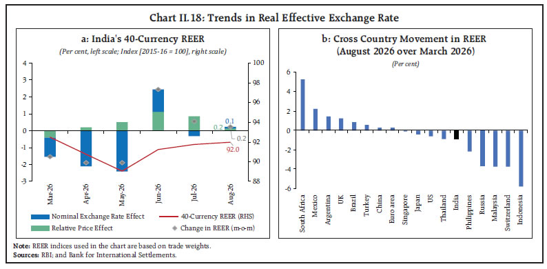
 The asset quality of SCBs strengthened further in Q1:2026-27 with the overall gross non-performing assets (NPA) ratio declining to 1.8 per cent in June 2026 from 2.3 per cent a year ago (Chart II.21a). The improvement spanned all major sectors, except for services and retail loans, where asset quality remained unchanged (Chart II.21b).
Banks’ non statutory liquidity ratio (non-SLR) investments (comprising CPs, bonds, debentures, and shares of public and private corporates) increased by around 2.9 per cent during H1:2026-27 (up to September 15), with an increase in investments in commercial papers due to higher returns (Chart II.22a). Growth in adjusted non-food bank credit (i.e., non-food bank credit plus banks’ non-SLR investments) accelerated to 17.6 per cent (y-o-y) in Q2:2026-27 (up to September 15) from 10.1 per cent in Q2:2025-26, (Chart II.22b). As on August 31, 2026, excess holdings of SLR securities by SCBs marginally moderated to 6.3 per cent of their net demand and time liabilities (NDTL) from 6.4 per cent at end-March 2026 as banks brought down their investment portfolio to fund credit demand (Chart II.23). Bank Credit: A Sectoral Perspective Sectoral trends8,9 indicate strengthening of credit growth across major segments. Sustained robust economic activity continued to underpin credit demand, supporting broad-based expansion in bank credit. Monetary policy was found to have heterogenous impact on sectoral credit growth (Box II.2). 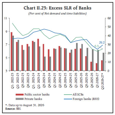
Box II.2: Bank Lending Channel of Monetary Policy: A Sectoral Approach Indian financial system continues to be bank-dominated. Bank credit as a proportion to GDP surged from 52.8 per cent in 2011-12 to 59.8 per cent in 2025-26. Therefore, given the importance of the banking sector, it becomes pertinent to understand the effectiveness of the transmission of monetary policy through the lending channel to various sectors of the economy. Under the current policy easing cycle, bank credit has inched up considerably across sectors. Demand conditions for credit have also been strong on the back of persisting buoyancy in domestic economic activity. In this milieu, it would be important to empirically decipher the response of sectoral bank credit to monetary policy shocks. Against this backdrop, the dynamic response of overall bank credit and credit to major sectors over 24 months following an unexpected policy rate change is examined using panel local projection technique (Jordà, 2005). Policy surprises are extracted using data on Overnight Index Swap (OIS) rates around RBI policy announcement dates, after controlling for current macroeconomic conditions (Lakdawala and Sengupta, 2025). Using monthly bank-level panel data of 40 banks for the period March 2014 - March 2026, the baseline specification for each horizon h = 0, 1, ..., 24 is given as under: 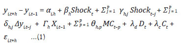 Where, yi,t represents credit growth for bank i in time t, yi,t+h – yi,t–1 is the dependent variable representing the cumulative credit growth for bank i from the pre-shock period to horizon h, αi,h are bank fixed effects at horizon h, Shockt is the exogenous monetary policy (target factor) shock at time t, and βh is the coefficient of interest, capturing the cumulative impulse response of bank credit to a one standard deviation monetary policy shock at horizon h. Plotting βh for h = 0, 1, ..., 24 traces the impulse response function. Shockt–j are lagged shocks controlling for prior monetary policy actions, Δyi,t–j controls for lagged values of the dependent variable, credit growth, Xi,t–1 is a vector of lagged bank characteristics (size, soundness, profitability, credit to deposits and borrowing ratio and asset quality) that can affect credit growth, MCt–p are lagged macroeconomic controls (nominal GDP growth and inflation) and Dt and Ct are dummies for demonetisation and COVID-19 pandemic, respectively. εi,t+h is the idiosyncratic error term clustered at the bank level. The lag length (p) is set to 12 months following the documented 6-to-18-month transmission lag in the Indian banking sector (Khundrakpam and Jain, 2012; Raj, et al, 2020). The impulse response of aggregate non-food credit to a one standard deviation expansionary monetary policy shock indicates that credit expands over the short to medium term, increasing by approximately 0.50 percentage points (pp) within the first six months, peaking to 0.8 pp around 13 months after the shock but becomes insignificant by the 15th month. Credit growth increases immediately following expansionary monetary policy shocks, reaches a peak after one year, and gradually reverts as balance sheets adjust (Chart II.2.1). 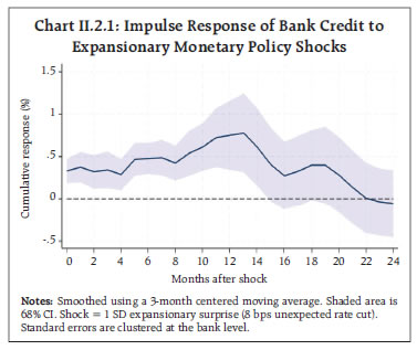
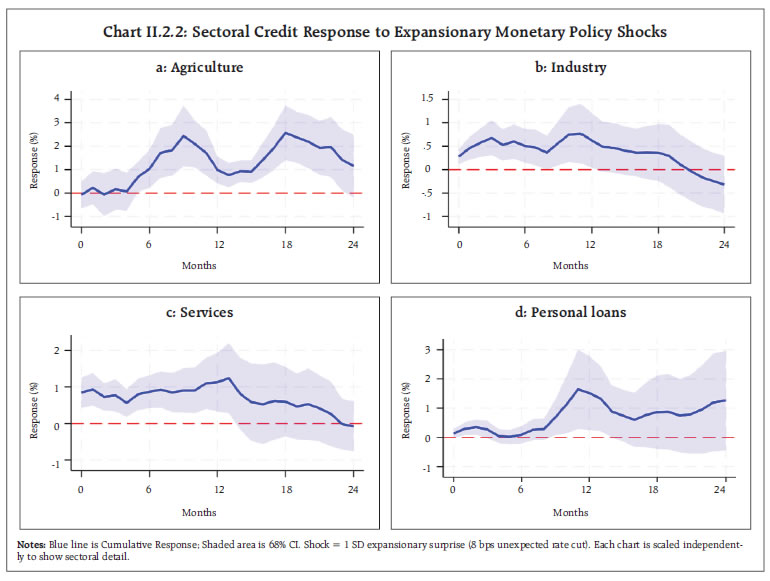 Across major sectors, the impact of the expansionary monetary policy shock is found to be heterogeneous. Credit to agriculture sector remains steady initially, before expanding from around 4th month onwards, reaching the peak in around 18 months. Industry and services sectors respond immediately to the monetary policy shock, with industry reaching its peak expansion earlier (around 10 months) than services (around 13 months), after which both sectors’ responses gradually taper off. The response of personal loans is found to be delayed, remaining flat over the first few months, but it follows a steeper expansion and peaks around 10th month, like industry (Chart II.2.2). References Jordà, Ò. (2005). Estimation and inference of impulse responses by local projections. American Economic Review, 95(1), 161–182. Khundrakpam, J. K., & Jain, R. (2012). Monetary policy transmission in India: A peep inside the black box, RBI Working Paper, WPS (DEPR): 11/2012. Lakdawala, A., & Sengupta, R. (2025). Measuring monetary policy shocks in emerging economies: Evidence from India. Journal of Money, Credit and Banking, 57(2-3), 407–437. https://doi.org/10.1111/jmcb.13144 Raj, J., Rath, D. P., Mitra, P., & John, J. (2020). Asset quality and credit channel of monetary policy transmission in India: Some evidence from bank-level data. RBI Working Paper, WPS (DEPR): 14/2020. |
| Table II.5: Credit Growth | | (Per cent, y-o-y) | | Sectors/Sub-Sectors | CAGR* | Post-COVID CAGR** | Mar-25 | Jun-25 | Aug-25 | Sep-25 | Dec-25 | Mar-26 | Jun-26 | Jul-26 | Aug-26 | | Bank Credit | 11.9 | 15.6 | 11.0 | 9.5 | 10.3 | 10.4 | 14.5 | 16.1 | 18.6 | 19.3 | 19.1 | | Sectoral Deployment of Bank Credit | | Agriculture (12.9) | 11.5 | 14.6 | 10.4 | 6.8 | 7.6 | 9.0 | 12.1 | 15.6 | 16.8 | 17.0 | 17.2 | | Industry (22.7) | 6.2 | 10.0 | 8.2 | 6.3 | 7.0 | 7.8 | 12.8 | 15.0 | 19.2 | 20.0 | 18.2 | | Micro and Small (5.3) | 12.2 | 16.4 | 8.9 | 19.2 | 20.8 | 22.0 | 30.4 | 32.7 | 23.0 | 22.6 | 23.0 | | Medium (2.3) | 16.3 | 17.3 | 18.5 | 13.2 | 13.3 | 14.5 | 20.4 | 21.8 | 30.3 | 30.5 | 31.8 | | MSMEs (7.6) | 13.3 | 16.7 | 11.8 | 17.4 | 18.5 | 19.7 | 27.3 | 29.3 | 25.1 | 24.9 | 25.5 | | Large (15.1) | 4.0 | 7.3 | 6.9 | 2.0 | 2.4 | 3.0 | 6.9 | 9.1 | 16.6 | 17.7 | 14.9 | | Infrastructure (7.2) | 5.4 | 5.2 | 2.8 | 0.8 | 3.5 | 5.0 | 7.2 | 9.2 | 10.9 | 10.2 | 10.2 | | Services (29.9) | 15.0 | 17.7 | 12.0 | 8.8 | 10.3 | 9.8 | 15.4 | 19.0 | 21.4 | 22.9 | 24.3 | | Services excluding NBFCs (19.6) | 13.0 | 17.4 | 14.4 | 11.7 | 13.5 | 12.7 | 15.6 | 15.4 | 16.5 | 17.2 | 18.4 | | NBFCs (10.3) | 20.3 | 18.2 | 7.4 | 3.1 | 3.7 | 3.9 | 15.1 | 26.6 | 32.2 | 35.7 | 37.5 | | Personal Loans (34.5) | 17.5 | 18.2 | 11.7 | 11.7 | 11.9 | 11.8 | 14.6 | 16.2 | 15.8 | 16.2 | 16.9 | | Personal Loans with unchanged Risk Weight (23.5) | 17.2 | 19.0 | 13.5 | 13.9 | 14.1 | 14.1 | 17.1 | 18.5 | 17.6 | 17.9 | 17.8 | | Housing (Including Priority Sector Housing) (16.4) | 15.9 | 16.8 | 10.7 | 9.6 | 9.7 | 10.1 | 11.1 | 11.5 | 11.0 | 11.3 | 11.1 | | Vehicle Loans (3.7) | 17.2 | 15.5 | 8.6 | 9.2 | 8.7 | 7.3 | 16.7 | 18.6 | 17.3 | 18.8 | 19.7 | | Education (0.8) | 8.8 | 16.8 | 15.1 | 14.4 | 14.6 | 14.0 | 14.8 | 13.4 | 13.3 | 13.7 | 13.2 | | Personal Loans with increased Risk Weight (11.0) | 18.1 | 16.6 | 8.3 | 7.5 | 7.5 | 7.1 | 9.8 | 11.7 | 12.0 | 12.7 | 15.2 | | Credit Cards (1.4) | 21.4 | 15.4 | 10.6 | 7.2 | 4.4 | 3.7 | 1.0 | 3.5 | 1.9 | 2.3 | 3.6 | | Other Personal Loans (8.5) | 19.1 | 16.5 | 7.5 | 7.1 | 7.6 | 7.4 | 11.5 | 12.8 | 14.2 | 14.7 | 15.0 | Notes: 1. Provisional data.
2. *: CAGR for the period between August 2016 to August 2026.
3. **: CAGR for the period between April 2022 to August 2026.
4. Figures in parentheses against each sector and sub-sectors denote share in total outstanding non-food credit as per the latest SIBC data.
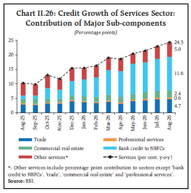
Source: RBI. | Industrial credit growth also picked up and it was above its compounded annual growth rate (CAGR) over the last 10-year period in H1:2026-27, supporting overall credit expansion (Table II.5). Services and personal loans continued to drive overall credit growth (Chart II.24). 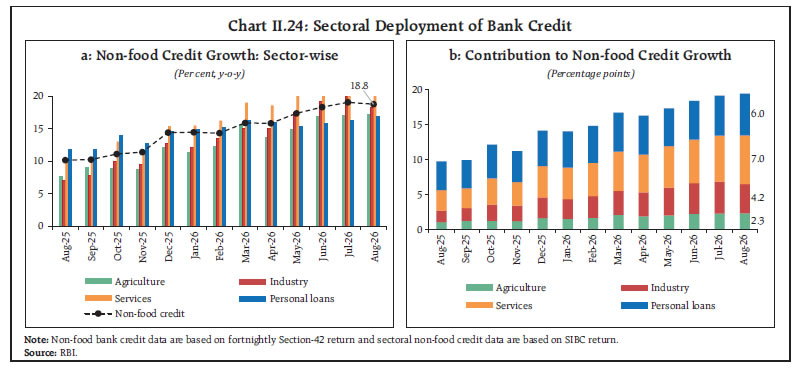 Credit to industrial sector registered robust growth during H1:2026-27, largely attributable to a sharp acceleration in credit to large industries. This was supported partly by corporates’ reduced recourse to market-based funding as its cost was higher on account of heightened geopolitical tensions. Credit to MSMEs10 continued on its double-digit growth trajectory, reflecting resilient credit demand including increased working capital requirements amidst global uncertainties and continued policy support. The policy support measures comprise the enhanced guarantee limit under the Credit Guarantee Fund Trust for Micro and Small Enterprises (CGTMSE) scheme, Emergency Credit Line Guarantee Scheme (ECLGS) 5.0, among others (Chart II.25). Among the major industrial sub-sectors, credit growth in infrastructure segment made a significant contribution to overall industrial credit expansion. 'Basic metal and metal products', ‘all engineering’ and 'chemicals and chemical products' also aided industrial growth (Chart II.25b). Within services sector, 'non-banking financial companies' (NBFCs) remained the largest recipient of bank credit during H1:2026-27, with improved availability following the withdrawal of the additional risk-weights effective April 1, 2025. Credit to services excluding NBFCs also expanded at a steady pace. Segments, such as trade and commercial real estate, recorded robust growth (Chart II.26). 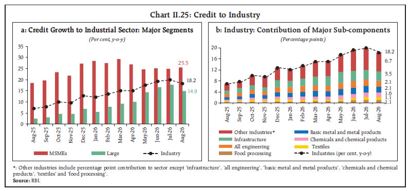
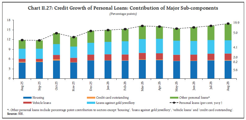
 Credit growth in personal loans segment remained buoyant during H1:2026-27, driven primarily by housing, loans against gold jewellery and vehicle loans. Housing loans, which account for nearly half of the personal loans, continued to grow at a steady pace reflecting robust real estate activity. Growth in loans against gold jewellery, albeit moderating from its peak in June 2025, remained elevated, which may be attributed to higher gold prices resulting in increased collateral valuation along with revised regulations effective from April 1, 202611. Vehicle loan growth accelerated sharply, nearly doubling vis-à-vis the previous year, on the back of persistent demand following the GST cut (Chart II.27). NBFC Credit: A Sectoral Perspective12 Credit extended by NBFCs exhibited robust expansion since August 2025, driven primarily by strong retail credit. The marked acceleration in credit growth to segments such as housing and gold, coupled with steady credit expansion in vehicle loans, drove the buoyant expansion in retail credit. Industrial credit growth softened, reflecting a moderation in lending to infrastructure, especially power sector, during H1:2026-27 (up to August). Credit growth in services sector remain strong despite some deceleration in recent months vis-à-vis last year (Table II.6). The continued buoyancy in retail lending underscored NBFCs' role in complementing the banking sector by catering to credit requirements of a diverse range of borrowers. II.3 Transmission to Lending and Deposit Rates Since the pause in the policy rate in February 2026, the weighted average domestic term deposit rates (WADTDRs) of scheduled commercial banks (SCBs) have moderated for both fresh and outstanding deposits by 40 basis points (bps) and 6 bps, respectively, in H1:2026-27 (till August), led by moderation in bulk deposit rates (Table II.7). At the same time, the weighted average lending rate (WALR) of banks have firmed up for fresh rupee loans, owing to strong credit demand. Bank credit growth outpaced deposit growth, leading to increased funding pressure. During H1 (till August), the WALR on fresh rupee loans increased by 21 bps, while it declined modestly by 3 bps for outstanding loans. During H1, the median 1-year marginal cost of funds-based lending rate (MCLR) rose by 21 bps. | Table II.6: Sectoral Credit Growth of NBFCs (including HFCs) | | (Per cent, y-o-y) | | Sector | CAGR* | Mar-25 | Jun-25 | Aug-25 | Sep-25 | Dec-25 | Mar-26 | Jun-26 | Jul-26 | Aug-26 | | NBFCs Credit | 9.8 | 11.6 | 11.2 | 10.0 | 13.3 | 13.8 | 14.1 | 14.3 | 14.9 | 15.8 | | 1. Agriculture and Allied Activities (1.3) | 14.1 | 6.0 | 5.1 | 5.1 | 5.2 | 9.4 | 15.8 | 18.1 | 18.0 | 17.4 | | 2. Industry (36.8) | 9.6 | 9.6 | 10.4 | 8.3 | 10.2 | 9.8 | 8.6 | 6.5 | 7.4 | 8.4 | | of which; | | | | | | | | | | | | 2.1 Infrastructure (33.4) | 8.7 | 9.2 | 9.7 | 7.2 | 9.4 | 8.9 | 7.0 | 5.0 | 6.2 | 7.2 | | of which; | | | | | | | | | | | | 2.1.1 Power (23.9) | 11.1 | 12.2 | 13.7 | 11.0 | 11.5 | 10.1 | 7.4 | 4.8 | 6.9 | 8.3 | | 3. Services (12.8) | 20.5 | 24.9 | 22.9 | 24.0 | 23.0 | 18.7 | 16.4 | 17.4 | 15.2 | 16.2 | | of which; | | | | | | | | | | | | 3.1 Transport Operators (3.0) | 13.3 | 12.8 | 11.0 | 10.8 | 9.4 | 9.1 | 11.0 | 10.9 | 10.7 | 10.7 | | 3.2 Trade (1.9) | 26.3 | 31.1 | 25.1 | 21.4 | 18.2 | 19.6 | 17.5 | 17.1 | 14.7 | 15.6 | | 3.3 Commercial Real Estate (1.7) | 13.8 | 5.4 | 10.5 | 11.3 | 8.9 | 24.7 | 33.5 | 30.9 | 22.3 | 21.8 | | 4. Retail Loans (43.7) | 10.6 | 13.4 | 14.3 | 13.6 | 16.8 | 17.9 | 20.2 | 20.3 | 21.4 | 22.0 | | of which; | | | | | | | | | | | | 4.1 Housing Loans (14.2)** | -5.2 | 5.4 | 4.2 | 3.8 | 10.0 | 10.5 | 10.2 | 11.4 | 11.9 | 12.1 | | 4.2 Vehicle Loans (10.5) | 18.0 | 16.8 | 15.6 | 15.0 | 14.9 | 14.2 | 15.2 | 15.2 | 15.1 | 15.4 | | 4.3 Loans against gold jewellery (6.0) | 39.9 | 32.2 | 40.6 | 46.8 | 50.7 | 61.2 | 73.8 | 68.9 | 68.5 | 69.1 | | 4.4 Consumer Durables (1.3) | 35.5 | 24.0 | 18.9 | 19.6 | 22.2 | 23.3 | 34.9 | 46.8 | 51.5 | 56.4 | | 5. Other Loans (5.4)*** | -8.0 | -8.0 | -19.5 | -21.3 | -4.6 | 4.2 | 5.1 | 17.4 | 19.7 | 20.3 | Notes: 1. Provisional data as reported on the last day of the month.
2. *: CAGR for the period between January 2023 to August 2026.
3. **: Housing loans data also include credit from HFCs.
4. ***: Other loans include credit from NBFCs other than agriculture, industry, services and retail loans, and non-housing loans from HFCs.
5. Figures in parenthesis represent share within total NBFCs credit.
6. Data include the impact of change in the nature of businesses of some NBFCs.
Sources: National Housing Bank (NHB) and RBI. |
| Table II.7: Transmission to Banks’ Deposit and Lending Rates | | (Basis points) | | Period | Repo Rate | Term Deposit Rates | Lending Rates | | WADTDR Fresh Deposits | WADTDR Outstanding Deposits | EBLR | 1-Yr. MCLR (Median) | WALR Fresh Rupee Loans | WALR Outstanding Rupee Loans | | | | Retail Deposits | Retail and Bulk Deposits | Retail and Bulk Deposits | Overall Effect | Interest Rate Effect# | | (1) | (2) | (3) | (4) | (5) | (6) | (7) | (8) | (9) | (10) | | Tightening Cycle May 2022 to Jan 2025 | +250 | 190 | 259 | 206 | 250 | 175 | 182 | 191 | 115 | | Easing Cycle Feb 2025 to Sep 2026* | -125 | -66 | -95 | -53 | -125 | -39 | -72 | -76 | -91 | | Memo | | H1: 2026-27* | 0 | 13 | -40 | -6 | 0 | 21 | 21 | 4 | -3 | | Jun – 2026 | 0 | 2 | 15 | 1 | 0 | -15 | 2 | 6 | -1 | | Jul – 2026 | 0 | 3 | -10 | 0 | 0 | 10 | -1 | 4 | 1 | | Aug – 2026 | 0 | -1 | -18 | -2 | 0 | 10 | 9 | -1 | -1 | Notes: 1. *: Data on WALR and WADTDR pertain up to August 2026.
2. Data on EBLR pertain to 32 domestic banks.
3. #: At constant weight of base period (January 2025).
WALR: Weighted average lending rate; WADTDR: Weighted average domestic term deposit rate; MCLR: Marginal cost of funds-based lending rate;
EBLR: External benchmark-based lending rate.
Sources: RBI; and staff calculations. |
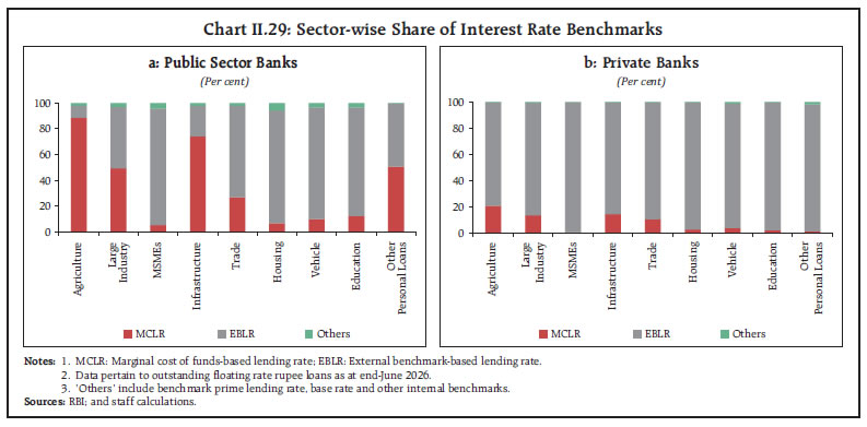
 In response to a cumulative reduction of 125 bps in the policy repo rate during February 2025 to August 2026, the WADTDRs for fresh and outstanding deposits have declined by 95 bps and 53 bps, respectively. On the lending side, WALRs for fresh and outstanding loans have declined by 72 bps and 91 bps, respectively. The share of the external benchmark-based lending rate (EBLR) linked loans in total outstanding floating rate loans of scheduled commercial banks increased from 67.6 per cent as at end-March 2026 to 68.2 per cent at end-June 2026. Consequently, the share of MCLR-linked loans declined from 30.2 per cent to 29.6 per cent. Public sector banks (PSBs) still have a significant proportion of their loans linked to MCLR (Chart II.28a), while private banks (PVBs) extend a large part of their loans at EBLR (Chart II.28b). The MCLR and other legacy rates – based on internal benchmarks and with longer reset periods – act as an impediment to faster policy transmission. PSBs have a high share of MCLR-linked loans in agriculture, infrastructure, other personal loans and large industry (Chart II.29a). The shares of MCLR-linked loans are lower for PVBs than those in PSBs (Chart II.29b). Bank group-wise, the transmission to WALRs on fresh and outstanding rupee loans of PVBs was higher than that of PSBs (Chart II.30a). The large share of EBLR-linked loans may have facilitated higher transmission in case of PVBs compared to PSBs. However, lending rates of PVBs remained above those of PSBs (Chart II.30b). The maximum pass-through to lending rates was witnessed among foreign banks, reflecting their higher share of EBLR-linked loans13 and a higher share of low-cost bulk deposits of lower maturity. 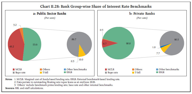
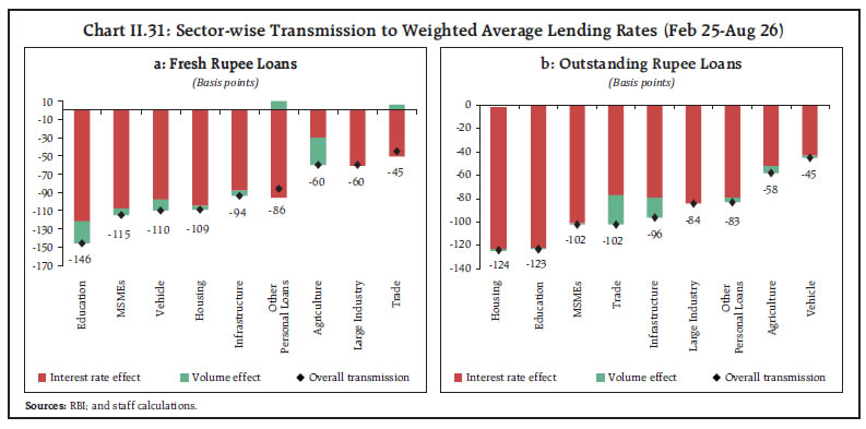
 Sectoral analysis shows that the transmission to lending rates has been heterogeneous due to varying proportions of credit portfolios linked to fixed and floating interest rates and differential spreads charged by banks. Furthermore, the shifts in volumes across banks/sectors towards higher/lower interest rate slabs could impact aggregate lending rates. The WALRs showed a broad based decline across sectors since February 2025. The volume effect, however, partially dampened transmission in other personal loans and trade in fresh loans, whereas it complemented in sectors such as agriculture and education, thereby enhancing transmission (Chart II.31). 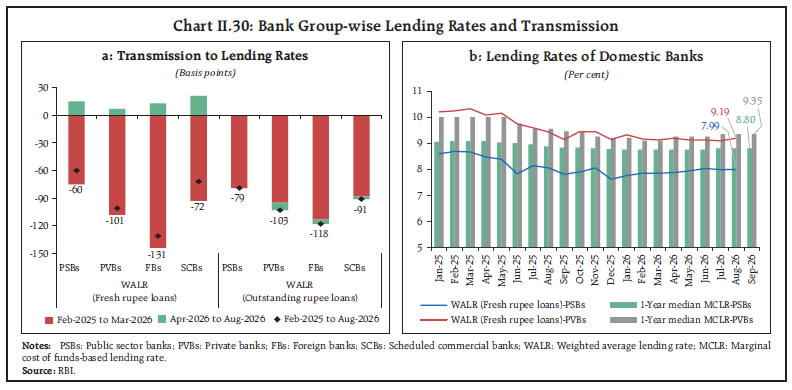
 For EBLR-linked loans, PVBs have increased their spreads (charged over the repo rate) for education, housing, MSMEs and vehicle loans, which dampened the extent of transmission (Table II.8). On the other hand, PSBs have reduced spread in education, MSME and vehicle loans, and increased it in other personal loans. For domestic banks, spread was higher in August 2026 over January 2025 for all sectors except education and vehicle loans. Through their extensive outreach and specialised lending activities across sectors, non-banking financial companies (NBFCs) substantially contribute to the transmission of monetary policy via the credit channel. Nevertheless, NBFCs typically charge higher lending rates compared to SCBs, mainly due to differences in the risk profile of borrowers, their funding structures, and cost of liabilities. During February 2025 to August 2026, lending rates of NBFCs moderated across sectors. The highest transmission in fresh lending rates was recorded in advances against gold followed by vehicle and MSME loans (Chart II.32). | Table II.8: Spread of Weighted Average Lending Rates on Fresh Rupee Loans* | | (Percentage points) | | Sectors | Jan-25 | Aug-26 | | Public sector banks | Private banks | Domestic banks | Public sector banks | Private banks | Domestic banks | | MSME Loans | 3.43 | 3.12 | 3.20 | 3.36 | 3.36 | 3.36 | | Personal Loans | | Housing | 2.09 | 2.44 | 2.34 | 2.09 | 2.69 | 2.44 | | Vehicle | 2.63 | 4.03 | 3.07 | 2.57 | 4.08 | 2.88 | | Education | 3.84 | 4.76 | 4.41 | 3.32 | 5.03 | 4.12 | | Other personal loans | 3.01 | 5.38 | 3.36 | 3.18 | 4.61 | 3.45 | Note: Other personal loans include loans other than housing, vehicle and education.
*: Calculated over the repo rate for loans linked to external benchmarks.
Sources: RBI; and staff calculations. |
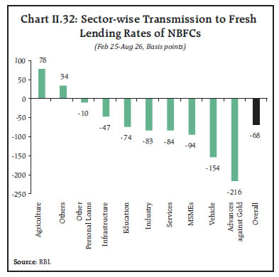 The Government of India reviewed the interest rates on various small savings instruments, which are linked to secondary market yields on G-secs of comparable maturities, and kept them unchanged for Q3:2026-27, marking 11 consecutive quarters with no change in rates. This has led to substantial positive spread of small saving instrument rates over their formula-based rates except for public provident fund (Table II.9). The widening gaps may be limiting the transmission of policy rates to banks’ deposit rates, especially during policy easing, because of the potential substitution effect. A large interest rate differential in favour of small savings could lead to migration of deposits away from banks, thus widening the credit-deposit gap in the banking system. II.4 Conclusion Financial markets conditions remained largely congenial during H1:2026-27, with intermittent bouts of volatility arising from geopolitical uncertainties, fluctuations in crude oil prices and capital flows. System liquidity remained in surplus for most of the period, aided by capital inflows under the Reserve Bank’s special swap facilities. Money market rates softened and remained largely range bound in line with the evolving liquidity conditions. Government bond yields softened before hardening in September, mainly reflecting global developments. Corporate bond yields moved in tandem with G-sec yields. Domestic equity markets gained in H1, supported by robust corporate earnings, and renewed buying by foreign investors. The Indian rupee experienced two-way movements with a depreciating bias, although the pace of depreciation moderated. Bank credit growth remained robust and broad-based across major sectors. The non-bank sources of finance also expanded. Transmission to deposit rates further strengthened in H1, while it moderated in the case of lending rates. Going ahead, liquidity management operations will be conditional on evolving domestic financial conditions, monetary policy decisions and the stance of monetary policy. | Table II.9: Interest Rates on Small Savings Instruments – Q3:2026-27 | | Small Savings Scheme | Maturity
(years) | Spread$
(Percentage point) | Average G-sec yield#
(Per cent) | Formula-based rate of Interest
(Per cent) | GoI Announced Rate of Interest
(Per cent) | Difference
(Basis points) | | (1) | (2) | (3) | (4) | (5) = (3) + (4) | (6) | (7) = (6) - (5) | | Savings Deposit | - | - | | | 4 | - | | Public Provident Fund | 15 | 0.25 | 6.97 | 7.22 | 7.1 | -12 | | Term Deposits | | | | | | | | 1 Year | 1 | 0 | 5.62 | 5.62 | 6.9 | 128 | | 2 Year | 2 | 0 | 5.82 | 5.82 | 7.0 | 118 | | 3 Year | 3 | 0 | 6.03 | 6.03 | 7.1 | 107 | | 5 Year | 5 | 0.25 | 6.44 | 6.69 | 7.5 | 81 | | Recurring Deposit Account | 5 | 0 | 6.03 | 6.03 | 6.7 | 67 | | Monthly Income Scheme | 5 | 0.25 | 6.41 | 6.66 | 7.4 | 74 | | Kisan Vikas Patra | 115 Months | 0 | 6.97 | 6.97 | 7.5 | 53 | | NSC VIII issue | 5 | 0.25 | 6.60 | 6.85 | 7.7 | 85 | | Senior Citizens Savings Scheme | 5 | 1.00 | 6.44 | 7.44 | 8.2 | 76 | | Sukanya Samriddhi Account Scheme | 21 | 0.75 | 6.97 | 7.72 | 8.2 | 48 | Note: Compounding frequency varies across instruments.
$: Spreads for fixing small saving rates as per the Government of India Press Release of February 2016.
#: Based on semi-annualised yield on G-sec of corresponding maturity for the period June 2026 – August 2026.
Sources: Government of India (GoI); Financial Benchmarks India Pvt. Ltd.; and RBI staff calculations. | _________________________________________________________________________________
III. Demand and Output Domestic economic activity exhibited resilience in H1:2026-27, despite continued global uncertainty. Real GDP posted a strong growth of 7.8 per cent in Q1:2026-27. Private final consumption remained healthy, supported by buoyant discretionary consumption. Revival in private capex and government’s continued focus on infrastructure spending strengthened investment activity. Manufacturing expanded at a robust pace, while services sector maintained its buoyancy. Looking ahead, weak monsoons, the prolonged West-Asia conflict, additional frictions in global trade and tighter global financial conditions may have an adverse bearing on both the demand and supply side of the economy. Domestic economic activity exhibited resilience in H1:2026-27, despite continued global uncertainty amidst the prolonged West-Asia conflict. The supply-side pressures were effectively dealt with proactive policy measures that ensured supply of key inputs for productive sectors. As per the National Statistics Office (NSO)’s estimates, real GDP recorded a growth of 7.8 per cent in Q1:2026-27 reflecting strong momentum in underlying economic activity. Aggregate demand remained strong on the back of both private consumption and investment. Net external demand also contributed positively to growth with rebound in merchandise exports and sustained buoyancy in services exports. On the supply side, both manufacturing and services sectors recorded strong growth in Q1. Going ahead, weak monsoon and El Niño may weigh on agricultural activity. Industry and services sectors are expected to continue benefitting from the Emergency Credit Line Guarantee Scheme 5.0 and the Transition Facilitation (Quality Control) Order 2026. Similarly, India’s growing network of bilateral free trade agreements (FTAs) augurs well for external demand, though uncertainties about additional tariffs on US imports, including those under Section 301, pose some risk. The risks from protracted West Asia conflict and financial market repricing due to changes in US monetary policy also require close monitoring. III.1 Aggregate Demand Aggregate demand conditions in the economy held up well in Q1:2026-27. As per the statistics released by the National Statistics Office, real GDP grew by 7.8 per cent, up from 6.9 per cent a year ago. Despite modest rise in domestic prices of select commodities, private final consumption expenditure (PFCE) remained healthy, while double-digit growth in gross fixed capital formation (GFCF) suggests a strong recovery in the capex cycle (Table III.1). Private final consumption contributed almost half of GDP growth in Q1:2026-27, though lower than 54.6 per cent a year ago. Strong growth in gross fixed capital formation (GFCF) also led to a sharp rise in its contribution to growth. By contrast, the contribution of government final consumption expenditure moderated in Q1. As real imports contracted and real exports rose sharply, net external demand was a positive contributor to GDP growth for the second successive quarter in Q1 (Table III.1 and Chart III.1a). The momentum of GDP – quarter-on-quarter (q-o-q) seasonally adjusted annualised growth rate (SAAR) – was placed at 6.5 per cent in Q1 (Chart III.1b). | Table III.1: Real GDP Growth | | (Y-o-y, per cent)^ | | Item | Annual | Quarterly | | Growth | Weighted Contribution* | 2025-26 | 2026-27 | | 2024-25 | 2025-26 | 2024-25 | 2025-26 | Q1 | Q2 | Q3 | Q4 | Q1 | | Private final consumption expenditure | 6.4 | 7.2 | 3.6 | 4.0 | 6.8 | 6.4 | 8.0 | 7.5 | 7.1 | | Government final consumption expenditure | 6.6 | 5.9 | 0.7 | 0.6 | 4.5 | 4.4 | 7.0 | 7.7 | 4.3 | | Gross fixed capital formation | 8.2 | 8.0 | 2.7 | 2.7 | 5.8 | 7.2 | 8.3 | 10.5 | 11.9 | | Exports | 4.9 | 6.4 | 1.1 | 1.4 | 6 | 9.7 | 6.2 | 3.9 | 12 | | Imports | 5.7 | 4.6 | 1.4 | 1.1 | 5.3 | 5.0 | 7.0 | 0.8 | -1.1 | | GDP at market prices | 7.2 | 7.8 | 7.2 | 7.8 | 6.9 | 8.1 | 7.7 | 8.6 | 7.8 | Note: *: Component-wise contributions to growth do not add up to GDP growth because change in stocks, valuables and statistical discrepancies are not included.
^: Unless specified otherwise, all discussions on growth rates in this chapter are on year-on-year (y-o-y) basis.
Sources: National Statistics Office (NSO); and RBI staff estimates. | The realised growth for Q1:2026-27 turned out to be higher than that projected in the Monetary Policy Report (MPR) of April 2026 (Chart III.2). This was mainly on account of a stronger than anticipated performance of gross fixed capital formation and net exports. III.1.1 Private Final Consumption Expenditure Private consumption growth in Q1:2026-27 remained strong at 7.1 per cent compared to 6.8 per cent during the same quarter last year, supported by buoyant discretionary spending. The rising purchasing power of households, buoyed by a prolonged phase of low inflation, stable employment conditions, tax rationalisation, and robust rabi production in previous quarters bolstered households' discretionary spending. Among major high frequency indicators, passenger vehicle sales recorded double-digit growth in April-July 2026. Demand for consumer durables increased at a healthy pace in Q1 and July-August, while growth in consumer non-durables remained subdued. The non-housing retail loans, which generally support discretionary spending, also increased at a robust pace. Slowdown in domestic air passenger traffic since February 2026 reflected price pressures amid the West Asia conflict. Tractor sales expanded at a robust pace during April-July, before remaining flat in August, which coupled with buoyant growth in two-wheeler sales during April-August, imply strong rural demand conditions. However, the increase in demand for work under the Viksit Bharat–Guarantee for Rozgar and Ajeevika Mission (Gramin) [earlier MGNREGA] in August- September 2026 due to weakening of agricultural activity reflects a shift of rural households towards low-paying jobs (Table III.2). 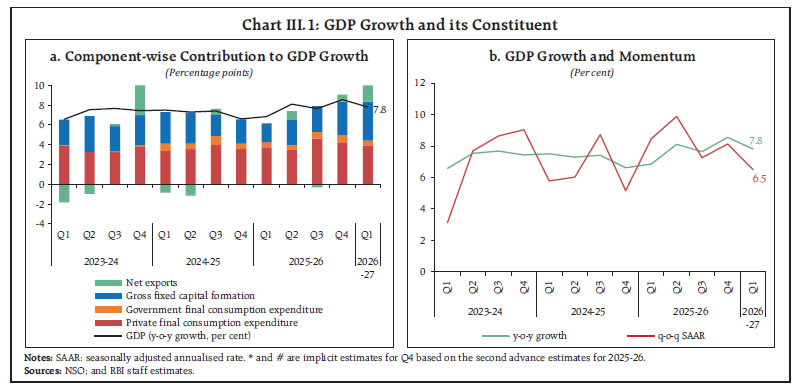
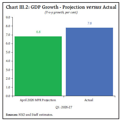 The extent of pass-through of input costs, impact of weak monsoon on rural income, and continued momentum in manufacturing and service sector activities will remain pivotal to the sustenance of overall PFCE growth. Government’s policy measures to support agriculture, resilient agriculture allied sectors, and a wider fiscal safety net through direct benefit transfers may help protect rural income and consumption. | Table III.2: Indicators of Consumption | | (Y-o-y growth, per cent) | | Indicators | 2024-25 | 2025-26 | 2026-27 | | Q1 | Q2 | Q3 | Q4 | Q1 | Q2 | Q3 | Q4 | Q1 | Jul | Aug | | Urban demand | | Domestic air passenger traffic | 5.6 | 7.3 | 11.4 | 12.0 | 5.3 | -2.1 | 1.7 | 0.6 | 1.2 | -4.7 | -9.0 | | Passenger vehicle sales (retail) | 5.0 | -2.0 | 8.7 | 3.8 | 2.9 | 5.1 | 20.9 | 23.7 | 22.3 | 19.1 | 16.1 | | IIP: Consumer durables | 11.1 | 9.5 | 8.5 | 4.8 | 2.8 | 3.1 | 4.3 | 2.1 | 8.0 | 12.0 | 11.1 | | Personal loans | 27.4 | 14.1 | 12.8 | 11.8 | 11.6 | 11.8 | 13.8 | 15.5 | 15.7 | 16.2 | 16.9 | | Vehicle loans | 13.6 | 11.0 | 10.4 | 9.3 | 8.9 | 8.3 | 13.9 | 17.6 | 17.5 | 18.8 | 19.7 | | Credit card outstanding | 23.3 | 20.0 | 16.9 | 11.6 | 8.7 | 4.6 | 3.7 | 2.3 | 2.3 | 2.3 | 3.6 | | Rural demand | | Tractor sales (retail) | -12.7 | -5.3 | 19.8 | -6.1 | 5.4 | 14.8 | 29.1 | 26.6 | 24.6 | 28.1 | 0.8 | | Two-wheeler sales (retail) | 13.0 | 5.3 | 12.9 | -3.5 | 4.0 | 0.5 | 19.1 | 26.3 | 15.3 | 28.3 | 19.7 | | IIP: Consumer non-durables | 4.0 | 3.5 | 3.9 | 3.0 | 1.5 | 1.8 | 0.1 | -0.1 | 1.8 | -0.8 | 2.1 | | Fertiliser sales | 2.4 | -7.3 | 0.4 | -9.6 | -14.7 | 30.6 | | | -47.2 | -18.9 | | | MGNREGA/VB-G RAM G work demand | -16.1 | -16.5 | 1.7 | 6.5 | 1.3 | -21.3 | -31.8 | -21.0 | -26.5 | -39.2 | 5.1 | | FMCG sales | | Rural | - | 5.7 | 9.1 | 8.3 | 8.4 | 7.7 | 2.9 | -0.8 | -5.1 | -7.8 | -8.0 | | Urban | - | 2.1 | 4.2 | 2.6 | 4.1 | 3.9 | 2.0 | 1.8 | -2.7 | -4.2 | -4.6 | | All India | - | 3.6 | 6.2 | 5.0 | 5.9 | 5.5 | 2.4 | 0.7 | -3.7 | -5.8 | -6.1 | | Sources: Directorate General of Civil Aviation (DGCA), Federation of Automobile Dealers Associations (FADA); NSO; RBI; Tractor and Mechanisation Association (TMA); and Ministry of Chemicals and Fertilisers (MoC&F); Ministry of Rural Development; NielsenIQ’s Retail Audit Service; and RBI staff estimates. | The July 2026 round of the Reserve Bank’s urban and rural consumer confidence surveys found moderation in households’ confidence for the current period. However, households are optimistic about their spending outlook for the year ahead amidst some concerns on the economic situation and employment (Table III.3). Labour market conditions continued to present a mixed picture in April-August 2026 (Chart III.3a). The worker population ratio and the labour force participation rate improved since June 2026 after three months of successive decline. The unemployment rate dropped in July and August 2026, after edging up in March-June. The workforce composition shifted towards regular salaried jobs, particularly in the secondary and tertiary sectors, with a decline in the share of self-employed in Q1:2026-27 over the previous quarters (Chart III.3b).1 III.1.2 Gross Fixed Capital Formation Gross fixed capital formation (GFCF) expanded by 11.9 per cent in Q1:2026-27 – the fastest pace in over three years. Investment activity was aided by both private and government capex. The share of GFCF in GDP improved to 34.3 per cent in Q1 from 33.1 per cent in the previous quarter. Buoyancy in investment activity was borne out by rising seasonally adjusted capacity utilisation in the corporate sector. A sharp surge in production and import of capital goods, robust credit demand and government’s capital outlay during July-August indicate continued buoyancy in investment activity during Q2. | Table III.3: Summary of Urban Consumer Confidence based on Net Responses | | Main variables | Current Perceptions | One year ahead Expectations | | May-26 | Jul-26 | May-26 | Jul-26 | | Economic Situation | -16.5 | -23.4 | 19.5 | 11.1 | | Employment | -14.4 | -21.9 | 21.8 | 15.1 | | Price Level | -90.7 | -92.7 | -71.5 | -74.9 | | Income | 0.9 | 1.9 | 47.1 | 45.8 | | Spending | 74.0 | 77.3 | 76.6 | 79.7 | | Consumer Confidence Index | 90.7 | 88.3 | 118.7 | 115.3 | Note: ‘Net response’ is the difference between the percentage of respondents reporting optimism and those reporting pessimism. It ranges between -100 and 100. Any value greater than zero indicates expansion/ optimism and values less than zero indicate contraction/ pessimism. Consumer Confidence Index = 100 + Average of Net Responses on the economic situation, income, spending, employment and the price level.
Source: Urban Consumer Confidence Survey, RBI. |
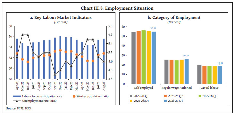 Revival in private-sector investment is gathering pace gradually as borne out by related indicators. Credit disbursal to large scale industry picked up sharply. Among major industries, credit to infrastructure; basic metal and metal products; engineering sector; chemical and chemical products; petroleum, coal products and nuclear fuels; and textiles recorded higher growth. Among major coincident indicators of investment in the construction sector, both steel consumption and cement production exhibited healthy growth in Q2:2026-27 so far (Table III.4). As per the CMIE data, private sector constituted 86.3 per cent of total new projects announced in H1:2026-27 vis-à-vis 68.7 per cent in H2:2025-26. The flow of resources to the commercial sector through various channels (banks/financial institutions, external commercial borrowings, initial public offerings, etc.) increased significantly in April-August 2026 from its level a year ago.2 The continued focus of public spending on transport, power, logistics and urban infrastructure is expected to crowd in private capex. Rise in capacity utilisation (CU) in previous few quarters augured well for new capacity additions that are required to meet domestic demand. Although CU in the manufacturing sector decreased sequentially in Q1, it was above its long-period average as well as the corresponding period’s level. The seasonally adjusted CU increased by 110 basis points from its level in the previous quarter and stood at 76.3 per cent in Q1:2026-27 (Chart III.4). III.1.3 Government Consumption Government final consumption expenditure (GFCE) in real terms grew by 4.3 per cent (y-o-y) in Q1:2026-27 compared to 7.7 per cent in the previous quarter (Table III.1). The gross fiscal deficit of the central government stood at 41.9 per cent of the fiscal year's budget estimates (BE) during April-August 2026, higher than 38.1 per cent, recorded during the corresponding period of the previous year. On the expenditure front, revenue expenditure of the central government (excluding interest payments and major subsidies) registered a growth of 12.5 per cent during April-August 2026 on a y-o-y basis, as compared to marginal contraction of 0.3 per cent during the same period of the last fiscal year (Chart III.5a). Expenditure on major subsidies (comprising food, fertiliser, and petroleum) of the Centre registered a double-digit growth of 24.4 per cent during April-August 20263 led by expansion in fertiliser and food subsidy. Interest payments by the Centre, however, contracted during April-August 2026, over the corresponding period of 2025-26. Capital expenditure of the Centre registered a y-o-y growth of 18.2 per cent during April-August 2026 (Chart III.5a). Accordingly, the quality of government expenditure improved as the ratio of revenue expenditure to capital outlay (RECO) declined in April-August 2026, boding well for infrastructure-led development4 (Chart III.5b). | Table III.4: Indicators of Investment Demand | | (Y-o-y, per cent) | | Indicators | 2025-26 | 2026-27 | | Q1 | Q2 | Q3 | Q4 | Q1 | Jul | Aug | | Import of capital goods | 14.3 | 8.5 | 14.7 | 12.9 | 25.6 | 25.4 | 23.6 | | IIP- Capital goods | 8.8 | 8.5 | 11.7 | 12.1 | 15.2 | 19.0 | 16.9 | | Finished steel consumption | 8.0 | 8.6 | 4.6 | 10.4 | 8.3 | 6.7 | 5.7 | | Cement production | 7.3 | 7.2 | 11.5 | 8.2 | 8.9 | 12.7 | 12.5 | | Sources: Directorate General of Commercial Intelligence and Statistics (DGCI&S); NSO; Joint Plant Committee; and Office of Economic Adviser. | On the receipts side, Centre’s gross tax revenue registered a growth of 6.5 per cent (y-o-y) during April-August 2026, attributable to growth in direct taxes. Direct tax collections registered a robust growth of 14.6 per cent (y-o-y) during April-August 2026, as compared to a contraction of 0.8 per cent during the corresponding period of last year. Robust growth in direct taxes is on account of double-digit growth in both corporation and income tax collections. Centre’s collections from indirect taxes contracted during April-August 2026, due to decline in goods and services tax (GST) revenue5 and revenue collected from union excise duties (Table III.5). It reflected GST rationalisation across key sectors and cut in excise duty on petrol and diesel. However, the GST collections by Centre plus States6 registered robust growth during April-September 2026 (Chart III.6). Net tax revenue, which largely represents Centre’s gross tax revenue adjusted for assignment to States, increased during April-August 2026 as assignment to States registered a strong growth during the period (Table III.5). 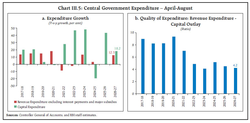
| Table III.5: Central Government's Tax Collections | | Item | ₹ thousand crore | Per cent | | BE | Actuals | Per cent of BE | Growth Rate (y-o-y) | | 2025-26 | 2026-27 | Apr-Aug 2025 | Apr-Aug 2026 | Apr-Aug 2025 | Apr-Aug 2026 | Apr-Aug 2025 | Apr-Aug 2026 | | A. Direct taxes | 2,520 | 2,697 | 693 | 794 | 27.5 | 29.4 | -0.8 | 14.6 | | of which: | | | | | | | | | | 1. Corporation tax | 1,082 | 1,231 | 229 | 265 | 21.2 | 21.5 | 2.1 | 15.4 | | 2. Income tax | 1,360 | 1,392 | 441 | 495 | 32.4 | 35.6 | -2.5 | 12.3 | | B. Indirect taxes | 1,750 | 1,707 | 651 | 638 | 37.2 | 37.4 | 2.7 | -2.0 | | of which: | | | | | | | | | | 1. GST | 1,183 | 1,025 | 454 | 439 | 38.4 | 42.8 | 5.0 | -3.4 | | 2. Custom duties | 240 | 271 | 83 | 107 | 34.6 | 39.3 | -11.9 | 28.2 | | 3. Union excise duties | 317 | 389 | 112 | 87 | 35.3 | 22.3 | 7.6 | -22.6 | | C. Gross tax revenue | 4,270 | 4,404 | 1,344 | 1,432 | 31.5 | 32.5 | 0.8 | 6.5 | | D. Assignment to States | 1,422 | 1,526 | 530 | 590 | 37.3 | 38.7 | 16.3 | 11.4 | | E. Net tax revenue | 2,837 | 2,867 | 810 | 838 | 28.6 | 29.2 | -7.3 | 3.4 | Note: BE: Budget Estimates.
Sources: Union Budget Documents; and Controller General of Accounts. | The central government’s non-tax revenue recorded a growth of 3.2 per cent during April-August 2026, primarily attributable to the surplus transfer of ₹2.87 lakh crore by the Reserve Bank in May 2026 (Chart III.7). The consolidated gross fiscal deficit of state governments and union territories7 is budgeted at 3.2 per cent of GDP for 2026-27, lower than the provisional estimates of 2025-26 (Table III.6). State governments continue to prioritise capital expenditure, as reflected in the decline in RECO ratio8 (Chart III.8). States’ capital expenditure is also supported by the central government through the ‘Scheme for Special Assistance to States for Capital Investment’, under which ₹2 lakh crore has been allocated for 2026-27.
| Table III.6: State Government Finances - Key Fiscal Indicators | | (Per cent of GDP) | | Item | 2024-25 (A) | 2025-26 (PA) | 2026-27 (BE) | | Revenue deficit | 0.6 | 0.7 | 0.2 | | Gross fiscal deficit | 3.2 | 3.4 | 3.2 | | Primary deficit | 1.5 | 1.8 | 1.5 | Note: Data pertain to 31 States/UTs.
A: Actuals; PA: Provisional Accounts; BE: Budget Estimates.
Sources: Budget documents of States/UTs and Comptroller and Auditor General (CAG) of India. | Data available for April-August 2026 indicate that the key deficit indicators of states, measured as a proportion of their respective budget estimates for 2026-27, were lower than in the corresponding period a year ago (Chart III.9a). This improvement is largely due to a lower growth in expenditure alongside a significant expansion in revenue receipts (Chart III.9b). Among the major components of revenue receipts, State Goods and Services Tax (SGST) collections registered strong growth at 15.2 per cent, while receipts from state excise duties and sales tax also remained buoyant.
| Table III.7: Government Market Borrowings | | (₹ crore) | | | H1:2025-26 | H1: 2026-27 | | | Centre | States | Total | Centre | States | Total | | Net Borrowings | 5,88,299 | 3,56,092 | 9,44,391 | 5,41,250 | 3,39,249 | 8,80,499 | | Gross Borrowings | 7,95,000 | 5,00,792 | 12,95,792 | 8,13,506 | 4,97,939 | 13,11,445 | | Source: RBI. | In the Union Budget for 2026-27, gross and net market borrowings of the Central Government through dated securities were pegged at ₹17.2 lakh crore and ₹11.7 lakh crore, respectively. Since the Budget presentation, switches of G-sec were conducted in March 2026, thereby reducing gross market borrowings of the Central Government to ₹16.0 lakh crore. During H1:2026-27, gross market borrowings raised by the Centre stood at ₹8.1 lakh crore, constituting 50.9 per cent of the revised gross market borrowings (Table III.7). The weighted average yield of issuances at 7.0 per cent in H1:2026-27 was higher than 6.6 per cent in H1:2025-26. The weighted average maturity of the issuances declined to 16.7 years in H1:2026-27 from 19.6 years in H1:2025-26. During H2:2026-27, the Government of India, in consultation with the Reserve Bank, has decided to borrow ₹7.9 lakh crore through dated securities. State Governments/Union Territories mobilised ₹5.0 lakh crore during H1:2026-27, as against the indicative calendar amount of ₹5.7 lakh crore. In order to bridge temporary mismatches between receipts and expenditures, the limit for Ways and Means Advances (WMA) for the Central Government was fixed at ₹2.5 lakh crore for H1:2026-27 and ₹50,000 crore for H2:2026-27. Currently, the aggregate WMA limit for States/UTs stands at ₹61,008 crore. III.1.4 External Demand Amidst the ongoing West Asia crisis and lingering trade policy uncertainty, global demand conditions continue to remain fragile. Strong demand for AI-related goods and the frontloading of consumer goods in anticipation of additional US tariffs after the expiration of temporary tariffs in July 20269, however, supported international trade. India's merchandise exports also rebounded and grew by 17.8 per cent in H1:2026-27 (April-August). With merchandise imports growing at a higher pace than exports, the merchandise trade deficit expanded to US$147.1 billion in H1:2026-27 (April-August) from US$ 123.9 billion in H1:2025-26 (April-August) (Chart III.10). Improvement in export performance was broad-based as the share of commodity groups with double-digit growth in H1:2026-27 (April-August) was 73.4 per cent vis-à-vis 16.2 per cent in H1:2025-26 (April-August). Petroleum products; engineering goods; electronic goods; organic and inorganic chemicals; and meat, dairy and poultry products were the main drivers of merchandise exports growth. Exports to the US remained resilient, primarily driven by electronic goods and engineering goods. Sectors that were a drag on exports included readymade garments of all textiles; ceramic products and glassware; fruits and vegetables; tobacco; and spices (Chart III.11a and b). 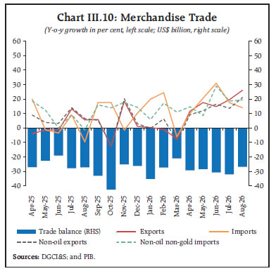
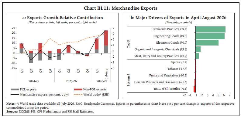 The growth in merchandise imports during H1:2026-27 (April-August) was driven by higher imports of electronic goods; petroleum, crude and products; machinery, electrical and non-electrical; fertilisers, crude and manufactured; and non-ferrous metals. By contrast, chemical material and products; pearls, precious and semi-precious stones; iron and steel; silver; and pulp and waste paper contributed negatively to import growth (Chart III.12). Gold imports at US$ 17.5 billion grew by 3.4 per cent during this period, while petroleum, crude and products imports grew by 22.4 per cent to US$ 95.6 billion, both reflecting the value impact due to steep rise in prices. Despite elevated trade uncertainty, both net terms of trade and income terms of trade improved in Q1:2026-27 vis-à-vis Q4: 2025-26, implying greater purchasing power of exports in terms of imports. As prices of key imports softened in June, net terms of trade in Q1 recouped from losses in the previous quarter (Chart III.13). India’s services exports growth remained robust at 10.9 per cent (y-o-y) in April-August 2026, led by software and business services (Chart III.14). India remains one of the top five service-exporting countries worldwide in terms of export growth in Q1:2026-27. Services imports also registered a strong growth in April-August 2026 on the back of higher transport and business services. Net services surplus increased by 7.3 per cent to US$ 85.8 billion in April-August 2026. Despite significant widening of the goods trade deficit, the current account deficit (CAD) at US$ 4.2 billion (0.5 per cent of GDP) in Q1:2026-27 was marginally higher than its level of US$ 3.4 billion (0.4 per cent of GDP) in Q1:2025-26 (Chart III.15). Services and remittance receipts continued to support the current account. There were net capital outflows of US$ 3.9 billion in Q1, as against net inflows of US$ 7.9 billion last year.10 Consequently, India’s foreign exchange reserves depleted by US$ 8.1 billion (BoP basis) during the quarter. As per preliminary estimates, CAD widened to US$ 7.0 billion in July 2026 from US$ 3.2 billion a year ago, driven by higher merchandise trade deficit and net income outgoes. 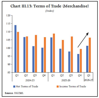
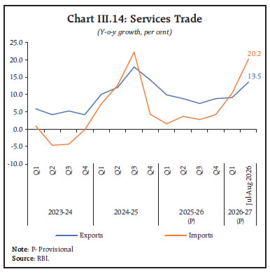
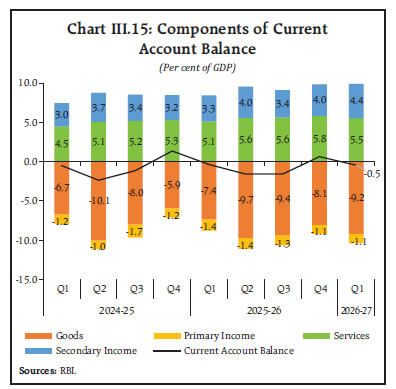 India’s gross inward foreign direct investment (FDI) and net FDI flows were higher in April-August 2026, both on y-o-y as well as sequential basis. A slowdown in the pace of outward FDI along with sustained higher gross FDI inflows supported net FDI flows. Financial services, communication services, computer services and manufacturing accounted for around 73 per cent of total FDI equity inflows during April-August 2026. In terms of origin, Singapore, Japan, Mauritius, The United Arab Emirates and the US were major sources of inward FDI to India, accounting for around 81 per cent of total inflows. Foreign portfolio investment (FPI) registered net outflows of US$ 8.9 billion during 2026-27 (up to September). After recording sustained outflows during the first quarter following geopolitical tensions in Middle East, FPI turned positive during June-August 2026 supported by measures taken by the RBI and the Government (Table III.8). FPI flows reversed again in September 2026 amidst rising global risk-off sentiment on re-escalation of Middle East tensions and rising US bond yields. External commercial borrowing (ECB) agreements during April-August 2026 (P) increased significantly by 93.4 per cent (y-o-y) to US$ 30.4 billion, partly attributed to the RBI’s concessional US dollar-rupee swap facility introduced in June 202611. Consequently, net ECB inflows to India12 grew by 55.9 per cent to US$ 7.3 billion during April-August 2026 from US$ 4.7 billion a year ago. In terms of utilisation, on-lending/ sub-lending accounted for the highest share (28.0 per cent), followed by general corporate purpose (13.8 per cent) and refinancing of rupee loans (11.9 per cent) during this period. As at end-August 2026, about 73.0 per cent of outstanding ECBs (excluding rupee and inter-company borrowings) were hedged by the Indian companies. Net inflows under non-resident deposits stood at US$ 119.2 billion during April-August 2026 (P), significantly higher than US$ 5.6 billion a year ago due to a surge in FCNR(B) deposits on account of RBI’s forex swap facility. During June 8 - August 31, 2026, gross inflows under the FCNR(B) deposit scheme stood at US$ 133.0 billion13. As of September 25, 2026, India’s foreign exchange reserves stood at US$ 747.6 billion which is equivalent to 10.9 months of goods imports and 96.1 per cent of the external debt outstanding as at end-June 2026. III.2 Aggregate Supply Aggregate supply – measured by real Gross Value Added (GVA) at basic prices – expanded by 8.2 per cent in Q1:2026-27 (8.7 per cent in the preceding quarter) despite headwinds after the onset of the West Asia conflict. Proactive measures undertaken by the Government to ensure adequate supply of key inputs supported growth in both manufacturing and services sectors (Chart III.16a and Table III.9). Supply-side measures included prioritisation of domestic supply and inventories, diversification of import sources of key inputs and targeted interventions to support the most vulnerable sectors. Some of these measures were subsequently withdrawn as supply-side pressures began to ease by end of Q1. The seasonally adjusted momentum of GVA moderated in Q1:2026-27 from the previous quarter (Chart III.16b). | Table III.8: Net Foreign Direct and Portfolio Investment | | (US$ billion) | | | 2024-25 | 2025-26 (Provisional) | 2026-27 (Provisional) | | Q1 | Q2 | Q3 | Q4 | Q1 | Q2 | Q3 | Q4 | Q1 | Q2 | | Net FDI | 6.2 | -2.8 | -2.8 | 0.4 | 5.2 | 2.1 | -5.1 | 4.5 | 3.1 | 10.7^ | | Net FPI | 0.9 | 19.9 | -11.4 | -5.9 | 1.6 | -5.7 | -0.2 | -13.5 | -9.6 | -0.3* | Notes: * implies that data for Net FPI to India for Q2:2026-27 sourced from daily data, published by NSDL; ^: Data for July-August 2026.
Sources: National Securities Depository Limited (NSDL) and RBI staff estimates. |
| Table III.9: Sector-wise Growth in GVA | | Sector | Annual | Quarterly | | Growth | Weighted Contribution | Growth | | (y-o-y, per cent) | (Percentage Points) | (y-o-y, per cent) | | 2024-25 | 2025-26 | 2024-25 | 2025-26 | 2025-26 | 2026-27 | | Q1 | Q2 | Q3 | Q4 | Q1 | | Agriculture and allied activities | 4.1 | 3.3 | 0.8 | 0.6 | 4.4 | 3.2 | 1.9 | 3.9 | 3.6 | | Industry | 9.4 | 7.8 | 1.8 | 1.6 | 7.3 | 10.1 | 7.6 | 6.4 | 7.7 | | Mining and quarrying | 13.5 | 7.1 | 0.3 | 0.2 | 12.4 | 21.6 | 3.3 | -2.9 | -2.4 | | Manufacturing | 10.0 | 8.8 | 1.5 | 1.4 | 8.3 | 10.0 | 9.0 | 7.9 | 9.2 | | Electricity, gas, water supply and other utilities | 2.8 | 2.1 | 0.1 | 0.1 | -1.8 | 3.8 | 1.9 | 4.8 | 8.9 | | Services | 7.4 | 9.3 | 4.5 | 5.7 | 7.6 | 8.9 | 9.6 | 11.0 | 9.7 | | Construction | 6.6 | 7.2 | 0.6 | 0.6 | 5.2 | 7.8 | 7.0 | 8.7 | 7.7 | | Trade, hotels, transport, communication | 7.0 | 11.3 | 1.0 | 1.6 | 9.8 | 10.6 | 11.7 | 12.9 | 8.5 | | Financial, real estate, ownership of dwelling, IT & professional services | 9.0 | 10.5 | 2.3 | 2.7 | 8.8 | 9.9 | 10.9 | 12.3 | 12.1 | | Public administration, defence and other services | 5.1 | 6.3 | 0.7 | 0.8 | 4.6 | 5.7 | 6.6 | 8.0 | 7.5 | | GVA at basic prices | 7.1 | 7.9 | 7.1 | 7.9 | 7.0 | 8.3 | 7.6 | 8.7 | 8.2 | | Sources: NSO; and RBI staff estimates. |
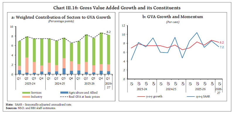 III.2.1 Agriculture Real GVA in agriculture and allied activities grew by 3.6 per cent in Q1:2026-27, lower than a year earlier. Robust growth in allied activities supported the overall growth in this sector. The shortfall and regional unevenness of Southwest monsoon and El Niño effects may pose some risks to both kharif and rabi output, though non-farm rural activities have shown greater resilience in recent years (Box III.1). The Southwest monsoon, after remaining weak in June, gained significant momentum subsequently, covering the entire country by July 9, 2026. Monsoon remained 1.0 per cent above the long period average (LPA) in July and supported kharif sowing. As of September 30, 2026, the cumulative rainfall was 12.6 per cent below the Long Period Average (Chart III.17a). In terms of spatial distribution, rainfall remained deficient compared to the LPA across all regions. As of September 30, 2026, the production-weighted rainfall index (PRN) stood at 90 per cent, suggesting a skewed rainfall distribution in major crop producing states (Chart III.17b). As of October 1, 2026, reservoir levels at 71.8 per cent remained below normal level14 (81.8 per cent) and last year’s level (90.3 per cent), due to erratic monsoon (Chart III.17c). Box III.1: Indian Agricultural Sector amidst Weather Shocks Rainfall shortfalls remain a major driver of year-to-year fluctuation in agricultural output. However, the rural economy is increasingly cushioned from erratic monsoon by resilient allied sector activities. Chand and Singh (2026) observe that for agricultural households possessing land up to one acre, wages contribute more than 55 per cent of household income, while crop production and livestock together contribute 36 per cent. This suggests that rural household incomes are increasingly supported by activities beyond crop production. Although annual estimates of value added are not available separately for rural and urban areas, historical benchmark estimates support the use of a broad rural-linked proxy. In 1999-2000, agriculture, forestry and fishing, mining and quarrying, and construction together accounted for about 59 per cent of total rural net domestic product (Central Statistical Organisation, 2007). This exercise therefore uses the sum of GVA of these sectors as an indicative proxy for rural-linked activity. Data available for both base years (i.e., 2011-12 and 2022-23) suggest that the non-agricultural component has become more important over time (Chart III.1.1). The growth-rate analysis below is calculated within the relevant published GVA base, with 2023-24 onward using the 2022-23-base series. Rainfall sensitivity differs across the two components of the proxy, viz., agricultural and non-agricultural (Chart III.1.2a). Agricultural growth suffers more in years of higher monsoon deficit, while growth in the non-agricultural component stays close to 6 per cent at every cut-off. In years of surplus rainfall, by contrast, agricultural growth averages 5.1 per cent, above the 4.3 per cent recorded in years close to the LPA. It is estimated that non-agricultural activity was the predominant contributor to growth in rural economic activity during years of rainfall deficiency exceeding 7 per cent, as against in other years. 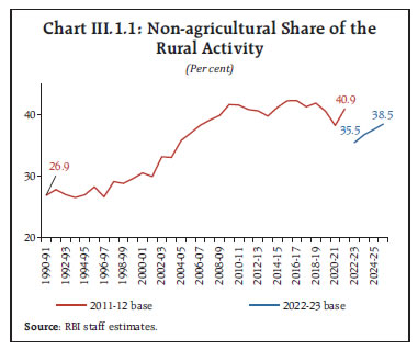 The same contrast is evident in the regression estimates (Chart III.1.2b). Over 1994-95 to 2025-26, a regression of annual growth of agriculture and allied activities on the rainfall shortfall from the long-period average gives a coefficient of (–) 0.40, statistically significant at 1 per cent. The shortfall measure explains about 39 per cent of the variation in agricultural growth. For the non-agricultural component, the coefficient is 0.01 but not statistically significant (Chart III.1.2b). The pattern is also stable across two equal sub-periods. Including a separate term for rainfall above the LPA leaves the shortfall coefficient for agriculture largely unchanged at (–)0.44, while the excess-rainfall term is small and not statistically significant at (–)0.12. A formal test rejects a symmetric response to deficient and surplus rainfall for agriculture (p value = 0.04) but not for the non-agricultural component. The asymmetry is not an artefact of the censoring implicit in the shortfall measure. The evidence on the declining role of rainfall in crop production is in line with Gupta et al. 2023. The factors that seem to have reduced the sensitivity of agricultural activity to rainfall shortfall include increased irrigation coverage, new weather resilient crop varieties, and diversification towards less water-intensive crops. At the same time, the composition of agricultural output has shifted towards allied activities. Over 1999-2000 to 2024-25, the coefficient for agriculture and allied GVA is (–)0.44 and significant at 1 per cent while the coefficients for milk, eggs, meat and fish as well as non-agricultural component are small and statistically insignificant (Chart III.1.3a). These estimates suggest that growth in these activities is less closely related to aggregate rainfall shortfalls than agricultural GVA. Rolling correlations of the absolute deviation of rainfall from the LPA with growth in agricultural GVA and the rural-linked activity proxy have generally become less negative since the mid-2000s (irrespective of the window-length), while remaining below zero throughout (Charts III.1.3b). 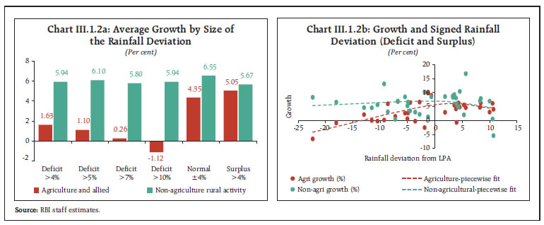
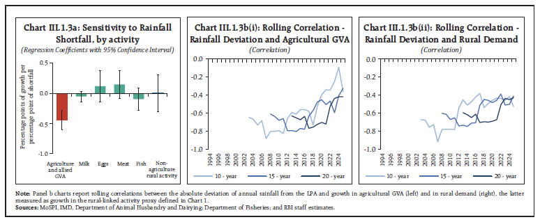 Summing up, empirical findings suggest that while rainfall shortfalls remain important for agricultural output, their association with allied activities and other rural-linked activity has moderated over time. Diversification across rural-linked activity and within agriculture has made the rural economy more resilient to rainfall shortfall. References: Chand, R., and J. Singh (2026). “Agriculture for Viksit Bharat: Strategies for Sustainable Growth and Transformation.” ICRIER Working Paper 434, July. Gupta, Kashyap; Sunil Kumar and Sarthak Gulati (2023), “Agriculture’s Dependency on Monsoon Rainfall in India”, RBI Bulletin, August. | As of October 2, 2026, kharif sowing was down by 1.0 per cent as compared to last year, while it remained above normal level by 1.0 per cent. The decline in kharif acreage was on account of lower sowing in rice, sugarcane and cotton, while sowing increased in pulses, coarse cereals and oilseeds (Chart III.17d). Rabi production may also face headwinds from low reservoir level due to deficient monsoon and above-normal temperatures associated with El Niño. 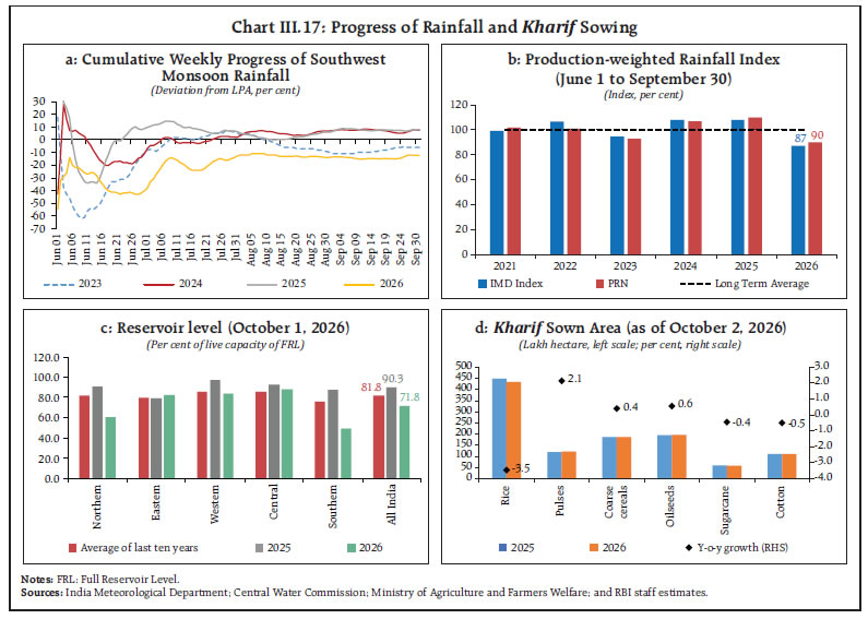 According to the third advance estimates of crops production for 2025-26, all major crops, except cotton, recorded an increase in production. Foodgrain output grew by 5.3 per cent to a record 3,766 lakh tonnes in 2025-26 (Table III.10). As per the second advance estimates, the production of horticultural crops reached 3,778 lakh tonnes in 2025-26, i.e., 1.9 per cent higher than the final estimates for 2024-25, driven primarily by higher output of banana; mangoes; potato; tomato; and non-TOP vegetables. The Government announced Minimum Support Prices (MSP) for kharif crops for the 2026-27 marketing season and rabi crops for 2027-28 marketing season. The increase in MSP ranged between 0.1-8.8 per cent across various kharif crops and 1.0-10.3 per cent across various rabi crops, with an intent to promote crop diversification and address demand-supply imbalances. III.2.2 Industry Industrial sector recorded a growth of 7.7 per cent in Q1:2026-27, which is higher than the previous quarter as well as a year ago. Real GVA growth in industry mainly reflected robust pace of activity in manufacturing and electricity segments, while the mining sector contracted in Q1 (Chart III.18a). A broad-based recovery was observed in the manufacturing sector with corporate manufacturing recording healthy revenue growth in Q1 amid rising cost pressures (Chart III.18b). | Table III.10: Agricultural Production in 2025-26 | | (Lakh tonnes) | | Crop | 2024-25 Final | 2025-26 | Variation in 2025-26 (Per cent) | | SAE | TAE | Over SAE 2025-26* | Over Final 2024-25 | | Foodgrains | 3,577.3 | 3,486.6 | 3,765.6 | 2.3 | 5.3 | | Kharif | 1,694.6 | 1,741.4 | 1,760.4 | 1.1 | 3.9 | | Rabi | 1,691.7 | 1,745.1 | 1,805.1 | 3.4 | 6.7 | | Summer | 191.1 | - | 200.1 | - | 4.7 | | Rice | 1,501.8 | 1,406.5 | 1,540.2 | 1.6 | 2.6 | | Wheat | 1,179.5 | 1,202.1 | 1,206.6 | 0.4 | 2.3 | | Coarse cereals | 639.2 | 639.3 | 744.7 | 7.2 | 16.5 | | Pulses | 256.8 | 238.7 | 274.1 | 2.7 | 6.7 | | Oilseeds | 429.9 | 410.0 | 430.6 | 1.4 | 0.2 | | Sugarcane | 4,546.1 | 5,002.0 | 5,000.6 | 0.0 | 10.0 | | Cotton # | 297.2 | 290.9 | 290.2 | -0.2 | -2.4 | | Jute & Mesta ## | 88.0 | 83.4 | 94.0 | 12.7 | 6.8 | Notes: *: SAE covers production of Kharif and Rabi crops only. Growth is calculated accordingly.
#: Lakh bales of 170 kgs each; ##: Lakh bales of 180 kgs each.
SAE: Second Advance Estimates. TAE: Third Advance Estimates.
Sources: Ministry of Agriculture and Farmers Welfare, GoI. |
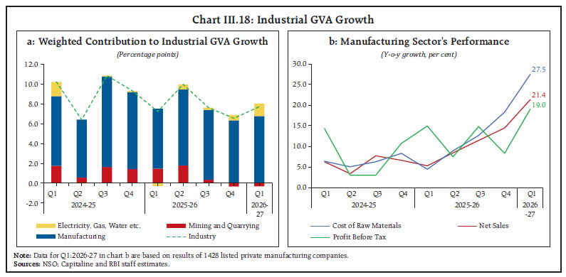 The index of industrial production (IIP) registered a healthy expansion of 6.7 per cent in April-August 2026 vis-à-vis 4.2 per cent in April-August 2025 (Table III.11). Manufacturing and electricity segments grew at a robust pace. Sectors having two-thirds of total weight within manufacturing reported higher production. Electrical, other transport equipment; motor vehicle; rubber & plastic products; and computer, electronics & optical products contributed to manufacturing growth. Mining sector slipped into contraction due to decline in fuel minerals; non-metallic minerals; and minor minerals. Activity in electricity, gas, water supply, and other utility services grew robustly in Q1:2026-27, after a prolonged phase of moderate growth. As per IIP data, electricity generation grew by 10.2 per cent during April-August 2026, while gas supply contracted marginally, probably reflecting input disruptions due to the West Asia Crisis. Electricity power generation from thermal; nuclear; and renewable sources reported higher production in April-July 2026, while hydro power generation contracted due to erratic weather conditions that reduced reservoir levels. In terms of regional demand, Southern region recorded a double-digit increase in electricity consumption during April-July 2026 (Table III.12). | Table III.11: Indicators of Industrial Activity | | (Y-o-y growth in per cent, unless indicated otherwise) | | | 2025-26 | 2026-27 | | Indicators | Q1 | Q2 | Q3 | Q4 | Q1 | Jul | Aug | Sep | | 1. PMI: Manufacturing (Index >50 indicates growth over previous month) | 58.1 | 58.7 | 56.9 | 55.4 | 54.6 | 53.5 | 52.8 | 55.1 | | 2. Index of Industrial Production (IIP) | 3.5 | 5.4 | 4.3 | 3.8 | 6.2 | 7.4 | 8.0 | | | 3. IIP: Mining & Quarrying | 3.5 | 14.0 | 2.2 | -1.8 | -1.2 | -0.9 | -5.6 | | | 4. IIP: Electricity & Gas Supply | -1.8 | 3.1 | -1.1 | 2.9 | 8.8 | 8.7 | 12.3 | | | 5. IIP: Water Supply, Sewerage & Waste Management | 8.2 | 6.9 | 4.9 | 5.7 | 6.0 | 7.4 | 6.3 | | | 6. IIP: Manufacturing | 4.1 | 4.7 | 5.2 | 4.7 | 6.9 | 8.2 | 9.0 | | | 7. IIP: Primary goods | 1.3 | 6.3 | 1.3 | 0.7 | 3.0 | 4.2 | 3.5 | | | 8. IIP: Capital goods | 8.8 | 8.5 | 11.7 | 12.1 | 15.2 | 19.0 | 16.9 | | | 9. IIP: Intermediate goods | 4.9 | 4.4 | 5.7 | 5.5 | 9.2 | 10.4 | 13.7 | | | 10. IIP: Infrastructure & construction goods | 6.1 | 10.1 | 9.8 | 9.3 | 7.2 | 8.0 | 6.4 | | | 11. IIP: Consumer durables | 2.8 | 3.1 | 4.3 | 2.1 | 8.0 | 12.0 | 11.1 | | | 12. IIP: Consumer non-durables | 1.5 | 1.8 | 0.1 | -0.1 | 1.8 | -0.8 | 2.1 | | | 13. Eight Core Industries (ECI) | 1.0 | 4.2 | 3.3 | 3.8 | 3.9 | 5.0 | 4.8 | | | 14. ECI: Steel | 9.4 | 15.1 | 10.7 | 11.1 | 5.1 | 1.9 | 3.4 | | | 15. ECI: Cement | 7.3 | 7.2 | 11.5 | 8.2 | 8.9 | 12.7 | 12.5 | | | 16. Electricity demand | -1.5 | 3.3 | -0.3 | 1.9 | 8.2 | 9.8 | 12.7 | | | Production of Automobiles | | 17. Passenger vehicles# | 3.4 | 4.2 | 19.1 | 11.3 | 16.8 | 26.4 | 25.7 | | | 18. Two wheelers | 0.7 | 10.8 | 15.0 | 20.7 | 22.8 | 24.2 | 15.2 | | | 19. Three wheelers | 9.8 | 18.5 | 34.7 | 32.4 | 39.1 | 30.0 | 21.5 | | | 20. Tractors | 12.7 | 14.6 | 31.5 | 37.2 | 14.4 | 6.7 | 13.6 | | Note: #: Does not include Tata Motors.
Sources: HSBC, S&P Global; CMIE; CEIC; NSO; SIAM; TMA; and RBI staff estimates. |
| Table III.12: Electricity Generation and Consumption | | (Y-o-y, per cent) | | Indicators | 2024-25 | 2025-26 | 2026-27 | | Q1 | Q2 | Q3 | Q4 | Q1 | Q2 | Q3 | Q4 | Q1 | Jul | Aug | | Electricity Generation | | Thermal | 12.0 | -1.4 | 0.0 | 0.3 | -8.1 | -1.5 | -5.4 | -1.0 | 7.5 | 12.2 | 11.8 | | Nuclear | 28.3 | 18.4 | 11.4 | 16.9 | 11.3 | -16.6 | -12.3 | 10.1 | 12.6 | 19.1 | 23.5 | | Hydro | 1.3 | 6.2 | 28.4 | 19.8 | 13.4 | 13.1 | 13.6 | 8.2 | -7.0 | -18.1 | -11.9 | | Renewables | 7.0 | 7.3 | 17.2 | 22.8 | 24.8 | 22.1 | 20.6 | 19.5 | 26.0 | 17.3 | 39.2 | | Electricity Consumption | | Northern region | 22.0 | 3.1 | 9.5 | 1.6 | -3.0 | -0.5 | -3.2 | 2.2 | 3.4 | 11.1 | 13.4 | | Western region | 5.5 | -6.7 | 0.4 | 4.4 | -0.3 | 7.0 | -1.3 | 0.8 | 9.2 | 6.4 | 8.1 | | Southern region | 3.3 | 0.8 | -2.3 | 3.1 | -1.3 | 2.9 | 2.9 | 1.6 | 14.0 | 14.0 | 19.9 | | Eastern region | 9.8 | 0.6 | 3.9 | 3.9 | -1.7 | 5.9 | 1.8 | 4.9 | 7.0 | 6.9 | 9.2 | | All-India | 10.2 | -0.7 | 2.6 | 3.2 | -1.5 | 3.3 | -0.3 | 1.9 | 8.2 | 9.8 | 12.7 | | Sources: Central Electricity Authority (CEA); and Power System Operation Corporation Limited (POSOCO). | Manufacturing purchasing managers’ index (PMI) remained in expansionary zone in H1:2026-27, although it moderated from H2:2025-26. The optimism in the new export orders inched up in September, whereas the outlook on the new orders remained steady. Stocks of finished goods increased, suggesting inventory build-up by manufacturing companies. The cost pressure on manufacturing firms remained elevated (Chart III.19a). III.2.3 Services Services sector expanded by 9.7 per cent and contributed nearly three-fourth to overall GVA growth in Q1:2026-27. The robust activity in services was also evident in PMI services, which remained in expansionary zone in Q2 (Chart III.19b). The momentum was driven by an upsurge in financial, real estate and professional services and trade, hotels, transport, communication, and services related to broadcasting (Chart III.20a). Construction activity also recorded a healthy growth of 7.7 per cent in Q1. Among the high frequency indicators of construction, cement production expanded at a robust pace during April-August 2026, whereas steel consumption growth moderated sequentially in July and August 2026 from its level in Q1 (Chart III.20b). 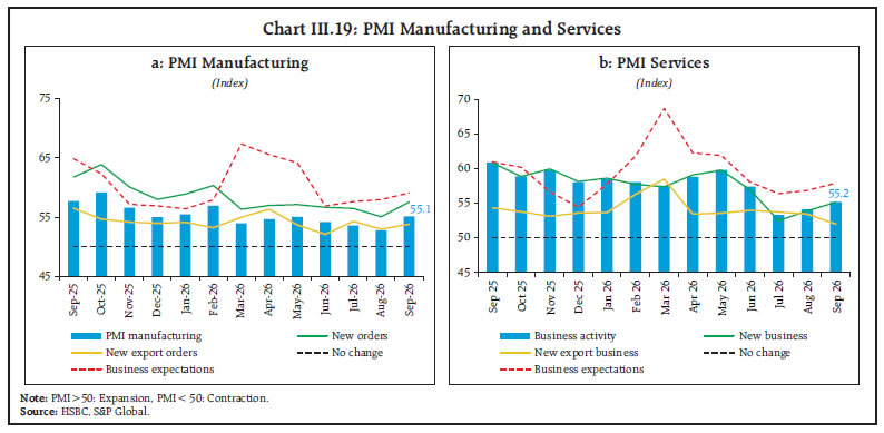
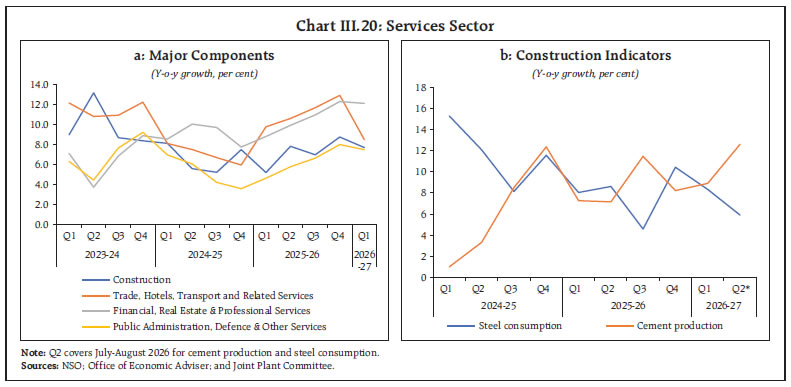 The growth in the real GVA of trade, hotels, transport, communication, and broadcasting services remained resilient at 8.5 per cent in Q1:2026-27 (12.9 per cent in Q4:2025-26). Among the transport indicators, domestic air traffic contracted mainly due to airlines scaling back their operations in response to surge in aviation turbine fuel price and pass-through of fuel prices impacting domestic travel. On the other hand, commercial vehicle sales and toll collection volume, indicators of road transport services, continued to grow at a robust pace in H1:2026-27 (April-July). After muted growth in Q1, gross GST collections surged by 15.4 per cent in July and 14.8 per cent in August 2026 indicating resilient business activity. Financial, real estate and professional services grew by 12.1 per cent in Q1:2026-27, contributing a major part to services sector growth (51.6 per cent) as well as to aggregate growth (37.0 per cent). Bank credit and deposit growth remained buoyant in Q2. Life insurance premium growth remained in double-digit in April-July 2026 (Table III.13). All these indicators suggest a continued resilient growth in financial services during Q2. Corporate sector performance in services sector improved in Q1:2026-27. Both GVA and operating profits of information technology (IT) firms improved, partly supported by favourable exchange rate movements. Non-IT services firms also recorded strong growth in both GVA and operating profits for the second successive quarter in Q1:2026-27 (Chart III.21). Growth in public administration, defence, and other services (PADO) – which also include education, health, recreation, and other personal services – grew at a stronger pace in Q1:2026-27 than a year ago. The centre’s revenue expenditure, excluding interest payments and subsidies, expanded by 11.4 per cent during April-July 2026. Services PMI dropped to 54.2 (average) in Q2:2026-27 from 58.7 in Q1:2026-27, albeit it remained in expansionary zone. Although new export business maintained similar optimism, outlook in new business worsened (Chart III.19b). After declining for two months from May 2026, the composite PMI rose to 55.9 in September 2026, compared to 54.3 in the previous month. Improvement in composite PMI was on the back of stronger increase in new order volumes reported by the private sector, though the pace of growth remained below the trend recorded in recent years. | Table III.13: Services Sector Indicators | | (Y-o-y growth, per cent) | | | 2025-26 | 2026-27 | | Indicators | Q1 | Q2 | Q3 | Q4 | Q1 | Jul | Aug | Sep | | 1. PMI: Services (>50 indicates growth over previous month) | 59.3 | 61.4 | 58.9 | 58.0 | 58.7 | 53.3 | 54.1 | 55.2 | | Construction | | 2. Steel consumption | 8.0 | 8.6 | 4.6 | 10.4 | 8.3 | 6.7 | 5.7 | | | 3. Cement production | 7.3 | 7.2 | 11.5 | 8.2 | 8.9 | 12.7 | 12.5 | | | Trade, Hotels, Transport, Communication and Services related to Broadcasting | | 4. Commercial vehicle sales | -0.6 | 8.3 | 21.5 | 18.9 | 18.3 | | | | | 5. Domestic air passenger traffic | 5.3 | -2.1 | 1.7 | 0.6 | 1.2 | -4.7 | -9.0 | -6.6# | | 6. Domestic air cargo | 6.6 | 4.9 | 6.8 | 12.5 | 9.1 | 4.2 | 3.5 | | | 7. International air cargo | 4.7 | 3.6 | 7.3 | 5.7 | 13.7 | 14.9 | 15.5 | | | 8. Freight traffic | 2.4 | 4.0 | 3.2 | 3.3 | 1.5 | 8.9 | 5.3 | | | 9. Port cargo | 5.6 | 5.9 | 13.1 | 4.0 | 6.1 | 8.8 | 8.4 | | | 10. Toll collection: volume | 16.2 | 14.7 | 16.7 | 12.4 | 14.0 | 15.5 | 11.7 | 16.4# | | 11. Petroleum consumption | 0.6 | 2.2 | 1.2 | 2.7 | -6.3 | 2.6 | -2.8 | | | 12. GST E-way bill | 20.5 | 23.1 | 19.4 | 15.7 | 12.4 | 6.0 | 7.7 | | | 13. GST revenue | 11.8 | 7.7 | 4.7 | 7.7 | 8.5 | 15.4 | 14.8 | | | Financial, Real Estate and Professional Services | | 14. Credit outstanding | 9.5 | 10.4 | 14.5 | 17.1 | 18.6 | 19.3 | 20.1 | 18.1* | | 15. Bank deposits | 10.1 | 9.5 | 12.7 | 16.2 | 13.3 | 15.4 | 18.6 | 17.3* | | 16. Life insurance premium | 4.3 | 10.7 | 24.9 | 21.7 | 16.6 | 20.7 | 33.1 | | | 17. Non-life insurance premium | 8.8 | 5.8 | 11.4 | 11.4 | 10.7 | 5.7 | 10.0 | | Note: * implies data as on September 15, 2026; # implies provisional data for September.
Sources: CEIC; NSO; HSBC, S&P Global; MOSPI; IRDAI; and RBI staff estimates. |
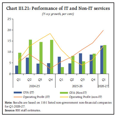 III.3 Conclusion Strong real GDP growth in Q1:2026-27, amidst global uncertainty and supply-side disruptions, signifies the inherent strength of the economy on the back of sustained focus on structural reforms, proactive policy responses, resilient macroeconomic fundamentals, and buoyant domestic demand. High frequency indicators available for Q2 suggest continued buoyancy in domestic economic activity, albeit with some moderation compared to Q1. Stable employment conditions, continued positive impact of tax rationalisation, congenial financial conditions, revival in corporate investment, and a pickup in goods exports are expected to support economic activity going forward. While a double-digit growth in GFCF reflects improving investment sentiment, sustenance of private consumption growth will be vital to broad-based recovery in private capex. Going forward, weak monsoons coupled with strong El Niño, protracted geopolitical tensions, rising international commodity prices, additional frictions in global trade and tightening of global financial conditions could adversely impact the outlook. _________________________________________________________________________________
IV. Prices and Costs Headline CPI inflation increased sequentially, rising above the target during June-August driven by a sustained positive price momentum. Higher food and fuel inflation led to this increase, reflecting adverse weather conditions and the sharp rise in energy prices following the West Asia conflict. Core inflation registered a pick-up with signs of generalisation in recent months. Going ahead, persistent supply-side pressures in food and volatile global energy prices pose risks to the domestic inflation outlook, particularly through second-round effects amid strong growth impulses. IV.1 Introduction The headline consumer price index (CPI) inflation1 has been increasing steadily in the period since the release of the previous MPR in April 2026. From 3.4 per cent in March 2026, headline inflation increased over successive months to 4.4 per cent in June (the first print above the inflation target in seventeen months) and further to 4.8 per cent in August (Chart IV.1a). The sequential pick-up in inflation witnessed since March was driven by a strong price momentum, which more than offset the favourable base effects in each month (Chart IV.1b).2 The momentum has been particularly strong since May. Among the major sub-components, food and fuel recorded sharp increases in y-o-y inflation over March levels (Chart IV.2a). Reflecting this, the contribution of food and fuel sub-components to headline inflation increased significantly (Chart IV.2b). The pick-up in food inflation was driven by unfavourable weather conditions and increasing fuel prices brought about by the sharp upturn in global energy prices following the West Asia conflict. Core inflation (CPI excluding food and fuel) also registered a pick-up, albeit by a lower magnitude upto July, reflecting limited pass-through of supply side pressures. In August core inflation accelerated to 4.2 per cent. 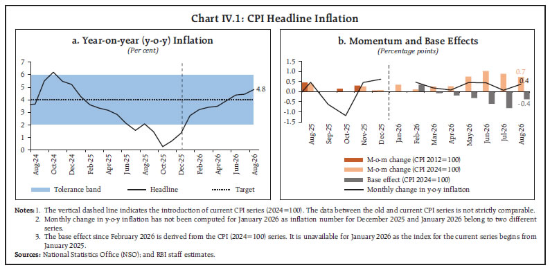
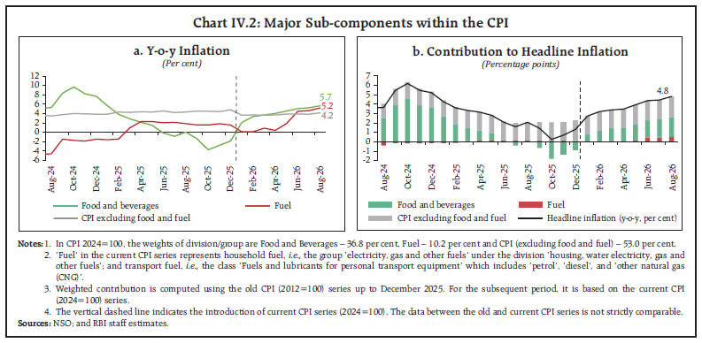 The April MPR projections had factored in risks from the West Asia conflict and adverse weather conditions as part of the baseline forecast. Reflecting this, the actual inflation outcomes remained broadly in line with the projections (Chart IV.3).3 Inflation for Q2:2026-27 so far (July-August) has turned out to be about 20 basis points (bps) higher than the quarterly average projection, as food price pressures have accentuated in recent months. The remainder of the chapter delves deeper into component-wise developments in inflation, statistical properties of observed inflation trends as well as determinants of inflation. IV.2 Developments across Major Components of the CPI CPI Food and Beverages Food and beverages inflation increased from 3.7 per cent in March to 5.7 per cent in August 2026, driven by items other than vegetables (Chart IV.4).
Of the 200-bps increase in food inflation in August over March, nearly 48 per cent was contributed by two sub-components, viz., animal protein4 and spices5, which together have a weight of about 36 per cent within the food and beverages division. The increase in inflation in animal protein primarily reflected rising input costs (Chart IV.5a). Higher feed and fodder costs, high transportation and packaging outlays, elevated energy prices, and heatwave-induced bird mortality contributed to the firming up of prices (Chart IV.5b). Inflation in spices rose steadily since January 2026 and touched 13.0 per cent in August, after being in deflation for a prolonged period.6 Ginger, dry chillies and coriander contributed the most to the increase. The emergence of El Niño conditions and deficient southwest monsoon have raised risks to overall food price outlook. However, robust domestic production in the previous year, comfortable foodgrain stocks7, conducive trade policy measures and proactive supply management provided some cushion, keeping the cumulative price build-up so far broadly in line with that of non-El Niño years (Chart IV.6). 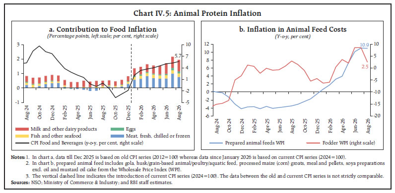
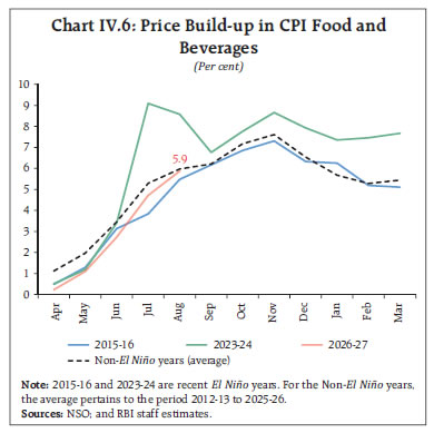 Among the major products, inflation in cereals and products8 increased to 2.8 per cent in August 2026 from -0.2 per cent in April amidst a pickup in rice prices on account of lower kharif sowing (Chart IV.7a). The build-up in cereals prices during 2026-27 (up to August) has also been above the historical average (Chart IV.7b). Pulses9 recorded a modest increase in y-o-y inflation, largely reflecting unfavourable base effects after remaining in deflation through most of 2025-26. Imports of key pulses from Myanmar, Brazil and Australia, along with government interventions in retail markets, helped keep prices at moderate levels.10 Inflation in oils and fats was lower at 7.8 per cent by August 2026 as compared to over 20 per cent a year ago (Chart IV.8a). Despite the moderation, elevated global edible oil prices amid increased diversion towards biofuel production in major producing economies continue to pose pressure on domestic prices. Domestically, tighter mustard seed arrivals amid steady export demand also kept mustard oil prices elevated (Chart IV.8b). However, reduction in basic import duty on crude palm, soybean and sunflower oils is likely to soften domestic prices.11
Vegetables12 inflation remained moderate, averaging 3.5 per cent (y-o-y) in H1:2026-27 so far (April-August 2026), supported by improved production and robust market arrivals.13 The price build-up in the Tomato, Onion and Potato (TOP) category was broadly aligned with its historical seasonal pattern while the increase in non-TOP vegetable prices remained below that observed in both El Niño and non-El Niño years (Chart IV.9). 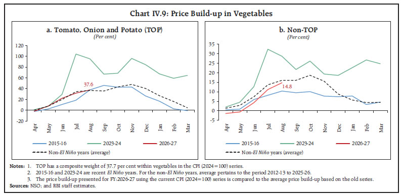 The impact of the deficient14 and uneven spatial rainfall distribution and lower kharif sowing15 on food prices is reflected in the recent high frequency retail price data in certain food items such as sugar and onion. Sugar16 prices increased by about 34 per cent since the first week of July to reach ₹65/ kg by late August, due to lower than anticipated domestic production, lower carry-over stocks, and precautionary stocking by market intermediaries17 (Chart IV.10). The government undertook targeted measures such as export restrictions, stock limits on dealers and bulk consumers, duty-free imports of up to 10 lakh tonnes of raw sugar, physical verification of stocks, and advancing the sugarcane crushing season to augment domestic availability and contain speculative pressures. Prices have since retreated in September. 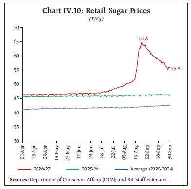 Onion prices have increased by about 84 per cent since end-June (up to September 30) due to depletion/ some spoilage of stored rabi stocks and concerns over the timing and quality of kharif arrivals amid uneven rainfall (Chart IV.11). Although onion prices exhibit a seasonal uptick during August-September before the arrival of the kharif crops, the magnitude of increase has been much higher this year than the historical average.
CPI Fuel Global crude oil prices ratcheted up since March 2026 along with an increase in the premium for refined products on account of extreme market tightness (Chart IV.12). Reflecting the partial pass-through of this increase, CPI fuel18 inflation went up from 0.4 per cent in April to 5.2 per cent in August. Among household fuel items included in CPI, domestic liquefied petroleum gas (LPG) prices were revised upwards by ₹60 per cylinder in early March 2026 and by a further ₹29 per cylinder in June, resulting in a cumulative increase of around 10.3 per cent. Kerosene and other fuel items also witnessed an increase in prices. Electricity prices, however, recorded a decline on a y-o-y basis on account of reduction in tariffs and provision of free or subsidised electricity in certain states (Chart IV.13a). Within transport fuel, retail prices of petrol and diesel were increased in four successive rounds during the month of May leading to a 7.5 per cent increase for petrol and 8.4 per cent for diesel (Chart IV.13b). The magnitude of domestic price increases was however moderate as compared to the increase in global prices (Chart IV.14). Part of the shock was absorbed by the Government by reducing the Special Additional Excise Duty on petrol and diesel by ₹10 per litre each in March to ease the burden on domestic consumers. After the initial surge, global oil prices have remained highly volatile with sharp two-way movements triggered by geopolitical developments. Amidst renewed uncertainty about the US-Iran negotiations, Indian basket crude oil prices increased from US$82 per barrel in July to around US$116 per barrel in September.19 Tightness in refined product markets also continues with low diesel inventories, higher stock drawdowns and the crude futures curve in backwardation.20 These conditions, along with elevated refined product margins, pose upside risks to domestic fuel prices if geopolitical disruptions persist.
Core CPI (CPI excluding Food and Fuel) Core inflation (CPI excluding food and fuel)21 increased from 3.7 per cent in April to 4.2 per cent in August 2026. Core inflation excluding precious metals22 registered a sharper increase from 2.2 per cent to 2.9 per cent during the same period (Table IV.1). Precious metals, which are part of the ‘personal care and effects’ sub-group, were a major driver of core inflation over the last year. During April-December 2025, gold and silver prices rose by 41.6 per cent and 66.3 per cent, respectively, accounting for about one-third of the overall core inflation during this period. After peaking in January 2026, precious metal prices have remained range-bound. In terms of sub-components, housing, restaurants and accommodation services, and clothing and footwear were the other major contributors to core inflation (Chart IV.15). Table IV.1: Exclusion-based Measures of Inflation
(Y-o-y, per cent) | | Period | CPI excluding food and fuel | CPI excluding food, fuel and precious metals | | Jul-25 | 4.2 | 3.2 | | Aug-25 | 4.3 | 3.1 | | Sep-25 | 4.5 | 3.1 | | Oct-25 | 4.5 | 2.6 | | Nov-25 | 4.4 | 2.4 | | Dec-25 | 4.8 | 2.4 | | Jan-26 | 3.7 | 2.1 | | Feb-26 | 3.7 | 2.1 | | Mar-26 | 3.7 | 2.1 | | Apr-26 | 3.7 | 2.2 | | May-26 | 3.9 | 2.3 | | Jun-26 | 3.9 | 2.5 | | Jul-26 | 3.9 | 2.7 | | Aug-26 | 4.2 | 2.9 | Note: Inflation numbers from July 2025 to December 2025 are based on the old CPI (2012=100) series, while those from January 2026 to August 2026 are from the current CPI (2024=100) series.
Sources: NSO; and RBI staff estimates. |
The pick-up in inflation up to July was primarily on account of higher inflation within goods category whereas services inflation remained moderate (Chart IV.16a). In August, however, services inflation also increased, indicating broadening of price pressures (Chart IV.16b). IV.3 Decoding the Inflation Dynamics Statistical properties Statistical properties provide useful insights into the nature of the inflation process, in terms of how generalised inflation is, and whether the underlying inflation differs from headline numbers. The distribution of CPI inflation on an average basis during 2026-27 so far (April-August) vis-à-vis 2025-26 indicates a positive skew, reflecting the disproportionately large contribution from precious metals for most months (Chart IV.17). In terms of the monthly trajectory, the increase in inflation during April-August 2026 was accompanied by a widening of inflation divergence across quantiles (Chart IV.18). The widening of inflation divergence across CPI groups is on account of an uptick in inflation in food, pan and tobacco, and personal transport groups.23
The recent uptick in inflation is also reflected in the CPI headline diffusion indices24 in August 2026, the weighted distribution of y-o-y headline inflation components shows a shift towards higher inflation categories (Box IV.1). 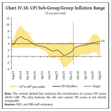
Box IV.1: Measuring Inflation Generalisation through the Diffusion Index When confronted with supply shocks, monetary policy responses are calibrated based on the assessment of second-round effects. If supply shocks are temporary, monetary policy often looks through them, whereas when there are signs of generalisation, policy acts to prevent inflation from becoming embedded in expectations. One critical challenge in this context is to gauge the extent to which inflation has become generalised. This can be assessed by examining whether the initial price pressures remain confined to the directly affected components or have spread to a wider set of items in the CPI basket. A useful measure of this generalisation is the inflation diffusion index, which captures the weighted distribution of item-level price changes in the CPI basket (de Soyres et al., 2026). An increase in the diffusion index in the high inflation categories indicates that price pressures are becoming more widespread across the consumption basket. This can be used along with the headline or core inflation numbers to understand the nature of inflation process. An increase in headline inflation accompanied by a low diffusion index for the high inflation categories is indicative of inflation driven by idiosyncratic supply shocks. On the other hand, surge in diffusion index in the higher inflation category along with the headline inflation number, indicates that inflationary pressures have become more broad-based and generalised. Many countries use diffusion indices alongside other measures of underlying inflation to understand the spread of inflationary pressures.25 Over the years, the Reserve Bank of India has also examined the distribution of item-level inflation using diffusion indices, inflation distributions and kernel density plots (RBI, Monetary Policy Report, various issues; Nadhanael and Pattanaik, 2010; Hasan et al, 2026). Against this backdrop, the box attempts to compile diffusion indices for inflation in India based on the revised CPI (2024=100) series. The diffusion indices are compiled for i) Headline CPI comprising all items; and ii) Core or CPI excluding food and fuel.26 The indices are constructed using weighted item-level year-on-year (y-o-y) inflation rates.27 Conceptually, diffusion indices represent the weighted share of items in the respective CPI basket, categorised into the following four buckets (intervals), aligning it with the inflation target and its tolerance band: i. Below 2 per cent; ii. Between 2 per cent and 4 per cent; iii. Between 4 per cent and 6 per cent; and iv. Above 6 per cent. The item-level y-o-y inflation rates are calculated using the following formulae:
The expenditure (CPI)-weighted diffusion index corresponding to inflation interval k is then calculated as: where ωi is the weight of the item i in the CPI basket and N is the number of the items in CPI basket (number of items = 358 for headline and 198 for CPI excluding food and fuel). The distribution of CPI inflation points to a progressive broadening of inflationary pressures. In August 2026, around 37 per cent of the CPI basket registered inflation above 4 per cent, as compared to 23 per cent in April 2026 (Chart IV.1.1a). The weighted share of the items in the CPI basket experiencing inflation below 2 per cent declined substantially with a notable rise in the weighted share of items experiencing inflation above 6 per cent. Distribution of core, i.e., CPI excluding food and fuel inflation also indicates a similar shift in distribution as in the case of headline inflation, albeit of a lower magnitude (Chart IV.1.1b). References: de Soyres, F., Pradhan, A., and Saijid, Z. (2026). Is the Inflation Process in Advanced Economies Different After the Pandemic? FEDS Notes. Washington, DC: Board of Governors of the Federal Reserve System. https://doi.org/10.17016/2380-7172.4024 Hasan, S., Sarkar, S., Anjanakrishna K and John, J. (2026). Diffusion Indices for Inflation in India: A Measure of Inflation Generalisation. Mimeo. Nadhanael, G. V., and Pattanaik, S. (2010). Measurement of Inflation in India: Issues and Associated Challenges for the Conduct of Monetary Policy. RBI Staff Studies. Reserve Bank of India. Reserve Bank of India. (n.d.). CPI Diffusion Indices: Various issues. Monetary Policy Reports. https://www.rbi.org.in/Scripts/PublicationsView.aspx?id=23426 | Statistical measures of underlying inflation such as the trimmed mean and the weighted median28, although increasing steadily during March to August 2026, remained lower than CPI excluding food and fuel inflation (Table IV.2). In terms of trajectory, they remain largely aligned with the conventional core inflation. Table IV.2: Measures of Underlying Inflation: Trimmed Mean Measures and Weighted Median
(Y-o-y, per cent) | | Month | 5% trimmed | 10% trimmed | 25% trimmed | Weighted Median | | Jul-25 | 2.7 | 3.0 | 3.1 | 3.0 | | Aug-25 | 2.9 | 2.9 | 2.9 | 3.0 | | Sep-25 | 2.5 | 2.6 | 2.7 | 2.7 | | Oct-25 | 1.9 | 2.2 | 2.4 | 2.4 | | Nov-25 | 2.0 | 2.2 | 2.4 | 2.5 | | Dec-25 | 1.8 | 1.9 | 2.1 | 2.1 | | Jan-26 | 2.3 | 2.2 | 2.0 | 2.0 | | Feb-26 | 2.4 | 2.5 | 2.1 | 2.0 | | Mar-26 | 2.7 | 2.4 | 2.2 | 2.0 | | Apr-26 | 2.7 | 2.6 | 2.3 | 2.0 | | May-26 | 3.1 | 3.0 | 2.6 | 2.3 | | Jun-26 | 3.7 | 3.6 | 3.3 | 2.7 | | Jul-26 | 3.8 | 3.5 | 3.4 | 3.1 | | Aug-26 | 4.2 | 4.0 | 3.7 | 3.5 | Note: Inflation numbers till December 2025 are based on the old CPI (2012=100) series, while from January 2026 are from the CPI (2024=100) series.
Sources: NSO; and RBI staff estimates. | Regional Trends in Inflation Turning to inflation trajectory across regions, both urban and rural areas have been experiencing an uptick in inflation since January 2026. Rural inflation consistently exceeded urban inflation during January-August 2026, which is largely attributable to the greater weight of ‘food and beverages’ that has witnessed a consistently higher inflation vis-à-vis other components during the same period (Chart IV.19). There was a marked divergence in inflation across states during April-August 2026 as compared to the corresponding period of last year. During 2025-26, average headline inflation was concentrated between 0-4 per cent. However, while 21 states in the current year registered average inflation in the range of 2-4 per cent, 13 states registered inflation in the 4-6 per cent range (Table IV.3). Only one state29 reported average inflation greater than 6 per cent during this period. 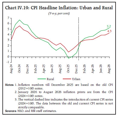
| Table IV.3: Distribution of Headline Inflation across States/UTs: Number of states1 | Headline Inflation Range
(Per cent) | 2025-26
(Apr-Aug)2 | 2026-27
(Apr-Aug)3 | | In Deflation | 0 | 0 | | Between 0 and 2.0 | 14 | 1 | | Between 2.0 and 4.0 | 16 | 21 | | Between 4.0 and 6.0 | 5 | 13 | | Greater than 6.0 | 1 | 1 | Notes: 1. Accounted for the unification of Daman and Diu with Dadra & Nagar Haveli and the formation of Ladakh as a Union Territory (UT) in the old CPI (2012=100) series.
2. Average headline inflation figures for April-August 2025-26 are based on old CPI (2012=100) series.
3. Average headline inflation figures for 2026-27 (April-August 2026-27) are from the CPI (2024=100) series.
Sources: NSO; and RBI staff estimates. | IV.4 Drivers of Inflation Trajectory This section analyses the evolution of inflation conditions based on the assessment of underlying factors. Imported Inflation The contribution of imported components to domestic inflation picked up in 2026 following the onset of the West Asia conflict. Imported inflation as per the Wholesale Price Index (WPI) (2022-23=100) registered a significant increase up to May 2026, with some pullback thereafter, driven by petroleum products (Chart IV.20). CPI imported inflation also remained elevated during this period, mainly due to higher precious metals prices, given the larger relative weight of precious metals in CPI.30 The extent of sequential increase in imported inflation in CPI since the onset of the West Asia conflict was lower than that in WPI, partly on account of delayed and partial price increases in petroleum products at the retail level. Cost Conditions Input cost pressures, as measured by WPI industrial raw materials and farm inputs inflation, rose sharply during March-May and remained elevated thereafter. The acceleration in industrial input costs was led by petroleum products, particularly aviation turbine fuel (ATF), high-speed diesel (HSD), naphtha, bitumen, furnace oil, and petroleum coke. The increase in farm input cost inflation was driven mainly by HSD, fertilisers, and nitrogen compounds (Chart IV.21). In the organised corporate sector, staff cost growth (y-o-y) in manufacturing accelerated in Q1:2026-27, following a moderation in Q4:2025-26 driven by strong momentum. In the services sector, y-o-y staff cost growth moderated during both Q4:2025-26 and Q1:2026-27, despite a positive momentum, on account of unfavourable base effects (Chart IV.22).
On the outlook for cost and price conditions, infrastructure and services firms expect both input cost and selling price pressures to abate during Q3:2026-27, as per the firms polled in the Reserve Bank’s enterprise surveys. Manufacturing firms expect a moderation in input cost pressures while also expecting an increase in selling prices. Salary outgo pressures are expected to increase for manufacturing firms during Q3:2026-27. In contrast, it is expected to ease for services and infrastructure firms (Chart IV.23). The Purchasing Managers’ Index (PMI) surveys indicate some sequential moderation in manufacturing firms’ cost pressures after the sharp increase following the onset of the West Asia conflict. Input price pressures reported by manufacturing firms eased gradually up to August 2026 after peaking in April. Output price pressures followed a broadly similar trajectory. Both input and output prices inched up in September. The manufacturing PMI input-output price gap turned positive in March 2026, indicating weak pass-through of input costs to selling prices. Although the gap narrowed from its March peak, it remained positive in August, suggesting some pent-up pass-through (Chart IV.24a). In the services sector, operating cost pressures eased gradually up to July before a mild pick-up in August 2026. Selling price pressures also moderated up to June but increased in July-August. Consequently, the services PMI input-output price gap narrowed significantly in August (Chart IV.24b). Similar trends were observed for Output and Input Producer Price Index (PPI)31 for manufactured products during April-August 2026. For most industry groups, pace of increase in input prices was faster than that of output prices, suggesting that the full extent of input price rise may not have been passed on to output prices (Chart IV.25). At the aggregate level, however, output prices rose faster than input prices driven by coke and refined petroleum products. Margins Food price margins32 have recorded a mixed trend in the recent period. Retail margins for cereals remained stable during April-September 2026. Margins for pulses remained stable until June before moderating during July-September. For TOP vegetables, margins picked up since April. In case of edible oils, margins peaked in May 2026 but remained range-bound thereafter (Chart IV.26).
In terms of the relative contribution of supply and demand factors in conditioning inflation dynamics, the evidence points towards the dissipation of both favourable supply and benign demand conditions, which led to increase in inflation in 2026-27 so far (Box IV.2). Box IV.2: What Drives Inflation in India? Disentangling Demand and Supply Factors Disentangling the relative roles of demand and supply factors in driving inflation is critical for an inflation-targeting central bank to calibrate appropriate policy response. Demand-driven inflation typically calls for monetary tightening, while supply-driven inflation creates difficult policy trade-offs as it is often accompanied by a slowdown in growth. In case of India, the recent experience of inflation significantly undershooting the target before a sharp reversal merits a thorough examination of the role of demand and supply factors in shaping the inflation dynamics. Empirical literature has adopted different approaches to disentangle the contributions of aggregate demand and supply conditions such as identifying the cyclical component of inflation by examining its relationship with economic activity as proposed by Stock and Watson (2020). Another approach is to explicitly decompose inflation into demand and supply-driven components using price and quantity information at the commodity or consumption-category level (Shapiro, 202433 and Shekhar, Kishore and Bhoi, 2023). More recently, Eickmeier and Hofmann (2025) have developed a structural factor model to identify aggregate demand and supply conditions using a broad set of inflation and real activity indicators. Their methodology exploits the common variation across a large number of macroeconomic series and identifies demand and supply factors through theoretically motivated sign restrictions on factor loadings. The demand factor is characterised by positive co-movement between inflation and economic activity, whereas the supply factor is associated with opposite movements in inflation and economic activity. This framework enables the construction of aggregate indicators of demand and supply conditions and facilitates an assessment of their contribution to inflation dynamics over time. This factor-based approach is applied to the Indian economy to identify indicators of aggregate demand and supply conditions and examine their role in the evolution of inflation in India. Compared with approaches that focus primarily on cyclical inflation or commodity-level price and quantity responses, the proposed framework incorporates information from a broader set of macroeconomic variables. Data The dataset includes a broad set of inflation measures including headline CPI, house price index, and other group/sub-group-wise inflation. The real-activity block includes GDP and expenditure components, gross and sectoral GVA indices, and other demand proxies such as diesel consumption and capacity utilisation. Other global price indicators like gold, copper, Brent crude oil and fertiliser prices are also included.34 Methodology The empirical strategy uses a factor model estimated by employing principal component analysis on quarterly macroeconomic time series data for India. Factor identification follows the standard supply-demand analysis based on randomly generated orthogonal rotations. The demand factor is identified as one that loads positively on inflation measures and real-activity measures. The supply factor is identified as one that loads negatively on inflation measures and positively on real-activity measures. Sign restrictions are imposed across key variables while allowing some variables to remain unrestricted. Once the demand and supply factors are identified35, Fry-Pagan median target approach is used to select accepted rotation closest to the median target. Results The findings indicate that the recent episode of inflation declining from H2:2024-25 to H2:2025-26 was driven by a weakening of demand as well as easy supply conditions (Chart IV.2.1 and Chart IV.2.2). Latest data for Q1:2026-27 show closing of negative demand conditions as well as waning of easy supply conditions. Demand factor converged to almost zero levels during Q1 as economic activity strengthened despite global shocks and emerging supply side pressures. As growth has surprised on the upside and inflation is showing early signs of generalisation, this indicates waning of favourable factors that kept inflation benign during 2025-26 and potential pressures going forward. References Eickmeier, S., and Hofmann, B. (2025). What Drives Inflation? Disentangling Demand and Supply Factors, International Journal of Central Banking, 21(3).
Shapiro (2004), A. (2024). Decomposing Supply and Demand Driven Inflation, Working Paper Series, Federal Bank of San Francisco. Shekhar, H., Kishore, B. and Bhoi B. B. (2023). Recent Inflation Dynamics in India: Role of Supply vis-à-vis Demand, RBI Bulletin, December. Stock, J. H., and Watson, M. W. (2020). Slack and Cyclically Sensitive Inflation. Journal of Money, Credit and Banking, 52(S2), 393-428. | The historical decomposition of inflation using a vector autoregression (VAR)36 model indicates that inflation firmed up since Q4:2025-26 as the impact of favourable supply shocks progressively waned while the contribution of fuel price shocks and exchange rate shocks increased (Chart IV.27). IV.5 Conclusion Headline inflation has increased steadily throughout 2026-27 (up to August), initially driven by higher food and fuel inflation but showing signs of broad-based price pressures in recent months. The impact of El Niño conditions and deficient southwest monsoon is increasingly reflected in food prices. Core inflation recorded a pick-up along with incipient signs of generalisation. Going forward, there is a material risk that supply-side pressures in food may remain unabated as weather uncertainties persist and global oil prices continue to remain volatile. In this context, generalisation of inflation through second-round effects remains a major risk from the firming up of demand conditions, given strong growth impulses. This is particularly pertinent as growth in credit and monetary aggregates remains robust (see Chapter II); therefore, stricter vigilance is required on the inflation front. _________________________________________________________________________________
V. Macroeconomic Outlook Amidst persistent geopolitical tensions, volatility in global commodity and financial markets and persisting trade uncertainty, India’s economic activity remains robust, supported by resilient domestic demand, strengthening investment and sound macroeconomic fundamentals. Headline inflation has firmed up in recent months, largely reflecting food and fuel price pressures, but with increasing evidence of generalisation. The outlook for growth and inflation is subject to uncertainties arising from external economic environment, commodity prices, weather events and global financial conditions. Against this backdrop, monetary policy remains focussed on maintaining price stability while supporting sustained economic growth. V.1 Key Developments since the April 2026 MPR Since the release of the Monetary Policy Report (MPR) in April 2026, the global economy has continued to navigate an uncertain environment precipitated by geopolitical tensions, evolving trade and tariff stipulations, volatile financial conditions, and rapid technological change. Despite these headwinds, global economic activity has remained resilient, with the International Monetary Fund (IMF) projecting global growth at 3.0 per cent in 2026 and 3.4 per cent in 2027.1 The inflation outlook, however, is of material concern with global headline inflation projected to rise from 4.1 per cent in 2025 to 4.7 per cent in 2026 by the IMF, suggesting that the disinflation process that was underway since early 2024 has reversed its course. Macroeconomic dynamics have been multi-paced across countries, reflecting the varying level of exposure to geopolitical developments, state of domestic demand conditions and extent of involvement in the ongoing technology-related investment cycle. Against this backdrop, monetary policy has been cautious in major economies with central banks balancing the risk of renewed inflationary pressures against concerns on slowing economic activity. Financial markets, meanwhile, have remained resilient, albeit with intermittent bouts of volatility in the wake of the prevailing uncertainty. Global equity markets have generally been supported by strong corporate earnings and optimism around technology-related investment, even as geopolitical uncertainties and macroeconomic data releases led to periodic corrections. Sovereign bond yields, particularly at longer maturities, have hardened across major economies amidst concerns over inflation, elevated public debt and large financing requirements. Global commodity prices have been volatile since April 2026, with the West Asia conflict induced initial surge moderating across some segments before renewed supply concerns triggered price pressures again since August. Energy markets were particularly sensitive to supply disruptions. Similarly, metal prices remained elevated amidst supply disruptions, supported by strong demand from infrastructure and technology-related investment, before moderating subsequently and rising again since August. The emergence of El Niño conditions has also added uncertainty to the outlook for agricultural production and food prices. Agricultural commodity prices, which were relatively stable after April, faced upward pressures from higher energy and fertiliser costs, adverse weather conditions and disruptions to trade and supplies. These developments were also reflected in currency markets with varying level of exchange rate adjustments across major economies. Fluctuations in the US dollar and evolving monetary policy expectations contributed to changing currency dynamics, while higher energy prices continued to exert pressure on some energy-importing economies. Amidst this volatile backdrop, the global economy has so far demonstrated resilience, although the interplay of geopolitical developments, inflationary pressures and financial market conditions will remain the key in shaping the outlook ahead. On the domestic front, economic activity remained robust in Q1:2026–27, with real GDP expanding by 7.8 per cent and real GVA by 8.2 per cent. Growth remains broad-based, with strong momentum in industry and services, while agriculture and allied activities also contributed positively. On the expenditure side, private consumption remained resilient and investment activity strengthened, with gross fixed capital formation registering a notable expansion. Headline CPI inflation increased from 3.5 per cent in April 2026 to 4.8 per cent in August, driven by sustained positive price momentum. Food inflation firmed up during this period and contributed significantly to the increase in headline inflation. Fuel inflation, which had remained subdued earlier, started increasing from May due to elevated international energy prices and their pass-through to domestic prices, albeit partially. Core inflation recorded only a modest increase till July before accelerating in August amidst signs of generalisation. Against this growth-inflation dynamics, the Monetary Policy Committee (MPC) considered it prudent to wait for the implications of prevailing uncertainties on growth and greater clarity on the inflation outlook to emerge before undertaking any policy action. Therefore, following the cumulative easing of 125 basis points during February to December 2025, the MPC left the policy repo rate unchanged at 5.25 per cent in its April, June and August 2026 meetings while retaining the neutral stance. Monetary Policy Committee Meetings: April 2026-September 2026 The MPC met for its first policy of the financial year in April 2026, amidst heightened geopolitical tensions arising from the West Asia conflict, which severely disrupted global supply chains, posing headwinds for India. The Indian economy, however, remained resilient, though elevated energy and commodity prices and disruptions in the Strait of Hormuz were expected to weigh adversely on domestic economic activity and inflation in 2026-27. Considering all these factors, real GDP growth for 2026-27 was projected at 6.9 per cent with downside risks while CPI headline inflation was projected at 4.6 per cent with upside risks. Core inflation was projected at 4.4 per cent for 2026-27. Recognising the supply-side nature of the shock and strong fundamentals of the domestic economy, the MPC considered it prudent to wait and unanimously decided to keep the repo rate unchanged at 5.25 per cent while retaining the neutral stance. At the June 2026 meeting, the continuing West Asia conflict posed risks to inflation and growth; nonetheless, domestic economic activity remained broadly resilient. Elevated energy and commodity prices and persistent supply disruptions were expected to weigh on growth. Consequently, real GDP growth projection for 2026-27 was revised downwards by 30 basis points (bps) to 6.6 per cent. Meanwhile, marginal pick up in headline CPI inflation in March and April, primarily due to higher food inflation and subsequent increases in retail fuel prices, raised inflationary pressures, leading to an upward revision of the CPI inflation projection for 2026-27 to 5.1 per cent. Core inflation was projected at 4.7 per cent for 2026-27. The MPC noted that while the risks to inflation have increased, it would be prudent to await for greater clarity on the evolving outlook. Accordingly, the MPC unanimously decided to retain the policy repo rate at 5.25 per cent along with the neutral stance. In the run up to the August 2026 meeting, the global economic outlook remained volatile as the relief from temporary ceasefire dissipated quickly. Domestically, risks to agriculture emanated from an erratic monsoon and El Niño conditions and supply-side measures were undertaken to mitigate the impact. Overall, the Indian economy demonstrated resilience, driven by better-than-expected consumption and investment demand, despite persistent global headwinds. Accordingly, real GDP growth projection for 2026-27 was revised slightly upwards to 6.7 per cent. On the inflation front, CPI inflation rose to 4.4 per cent in June 2026 after remaining below the target of 4.0 per cent for 16 consecutive months, but was 30 bps lower than projections, prompting a downward revision of the 2026-27 inflation projection to 5.0 per cent. The core inflation was also projected lower at 4.3 per cent for 2026-27. The MPC observed that the rise in headline inflation was mainly driven by supply-side pressures and considered it appropriate for greater clarity to emerge on the inflation outlook before taking policy action. Accordingly, the MPC unanimously voted to keep the policy repo rate unchanged at 5.25 per cent and retained the neutral stance. Nevertheless, the MPC pointed out that any policy action would also consider the recalibration of policy rates in line with the evolving growth-inflation dynamics, especially normalisation of the underlying inflation from its earlier benign levels. The Indian MPC’s unanimous voting pattern stands in contrast to the diversity in voting witnessed in many other central banks (Table V.1). Monetary policy decisions remained divergent across economies based on domestic conditions, although a tilt towards hawkish pivot is visible. Among the Advanced Economies (AEs), while policy rate remained broadly unchanged, dissent among the members was more pronounced. Japan and the UK witnessed voting disagreements in all their meetings, while the US saw dissent in two out of four meetings with a rate hike in its latest meeting. Among the Emerging Market Economies (EMEs), pivot towards hiking is visible for some although Brazil and Hungary have reduced their policy rates by 100 bps and 75 bps, respectively, in view of high real policy rates. | Table V.1: Monetary Policy Committees and Policy Rate Voting Patterns | | Country | Policy Meetings: April 2026 - September 2026 | | Total meetings | Meetings with full consensus | Meetings without full consensus | Variation in policy rate (basis points) | | Brazil | 4 | 4 | 0 | -100 | | Chile | 4 | 4 | 0 | 0 | | Colombia | 4 | 1 | 3 | 100 | | Czech Republic | 4 | 3 | 1 | 25 | | Hungary* | 6 | 3 | 2 | -75 | | India | 3 | 3 | 0 | 0 | | Japan | 4 | 0 | 4 | 50 | | South Africa | 3 | 1 | 2 | 50 | | Sweden | 4 | 4 | 0 | 0 | | Thailand | 3 | 3 | 0 | 0 | | UK | 4 | 0 | 4 | 0 | | US | 4 | 2 | 2 | 25 | Note: 1. Minus sign indicates a reduction in policy rate.
2. *: Total number of meetings happened is six. However, the minutes of last meeting (September 22, 2026) are not published to date.
Sources: Central bank websites. | Factors conditioning the Macroeconomic Outlook Macroeconomic developments pertaining to economic activity and inflation during H1:2026-27 are analysed in chapters III and IV. Going forward, the outlook is based on a set of baseline assumptions. First, assumption on crude oil price has been revised up to US$95 per barrel for the second half of 2026-27 from US$85 per barrel for 2026-27 in the last MPR (Table V.2). This makes the alternate scenario presented in MPR April 2026 as our baseline with a $10 per barrel rise in oil price assumption over 2026- 27 and 2027-28. International crude oil prices peaked in April 2026 primarily because of severe supply shock caused by the West Asia conflict. Following the signing of Memorandum of Understanding between the US and Iran in June, oil prices eased and reached around US$83 per barrel in July 2026. After the ceasefire violations and the consequent collapse of the US-Iran agreement, prices began to firm up in August and further escalated in September. The Brent futures curve, however, remained in backwardation, with expectations of prices easing in future (Chart V.1a). The upward pressure on prices was mitigated to some extent due to destocking of crude oil inventory by several countries, which has witnessed sharp depletion since Q4:2025-26, with minimal support to prices expected in the months ahead. With steady increase in production, crude oil inventory is expected to be replenished in the second half of 2026-27 that might keep demand and price pressures high (Chart V.1b). | Table V.2: Baseline Assumptions for Projections | | Indicator | MPR April 2026 | MPR October 2026 | | Crude Oil | US$85 per barrel during 2026-27 and US$75 per barrel during 2027-28 | US$95 per barrel during H2: 2026-27 and $85 per barrel during 2027-28 | | Exchange rate | ₹ 94/US$ during 2026-27 | ₹ 95/US$ during 2026-27 | | Monsoon | Normal for 2026-27 and 2027-28 | Below normal for 2026-27 and normal for 2027-28 | | Global growth | 2.9 per cent in 2026
3.0 per cent in 2027 | 3.0 per cent in 2026
3.4 per cent in 2027 | Fiscal deficit
(per cent of GDP) | To remain within BE 2026-27
Centre: 4.3
Combined:6.8 | To remain within BE 2026-27
Centre: 4.3
Combined: 7.0 | | Domestic macroeconomic/ structural policies during the forecast period | No major change | No major change | Notes: 1. The assumption on oil is based on Brent Crude.
2. The exchange rate path assumed here is for the purpose of generating the baseline projections and does not indicate any ‘view’ on the level of the exchange rate. The Reserve Bank is guided by the objective of containing excess volatility in the foreign exchange market and not by any specific level of and/or band around the exchange rate.
3. BE: Budget Estimates.
4. Combined fiscal deficit refers to that of the Centre and States taken together.
Sources: RBI estimates; Budget documents; and International Monetary Fund (IMF). | Second, the nominal exchange rate of the Indian rupee (₹) remained in the range of ₹92–97 per US dollar during April–September 2026 (Chart V.1c). The rupee depreciated towards the end of April driven by portfolio outflows that reflected a risk off sentiment towards EMEs under heightened uncertainty. Subsequently, the rupee reversed its trend, supported by the easing of geopolitical tensions and the announcement of measures by the Reserve Bank of India to attract foreign capital flows including USD-INR swap window for FCNR(B) deposits and foreign investment in government securities. The Indian rupee subsequently weakened in early July in tandem with rising crude oil prices, but has since remained range-bound. Considering the volatility of the US dollar and fluctuations in global capital flows, the baseline assumption for the exchange rate has been revised to ₹95 per US dollar as against ₹94 in the April 2026 MPR. 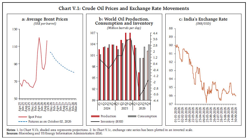 Third, according to the IMF, global economic growth is projected at 3.0 per cent in 2026 and 3.4 per cent in 2027, lower than 3.5 per cent registered during 2025 (Chart V.2). The prolonged conflict in West Asia continues to pose significant downside risk, with the potential to exacerbate supply-chain disruptions, and tighten financial conditions. AEs are projected to grow at 1.7 per cent in 2026, marginally lower than 1.9 per cent in 2025, while growth in EMEs is expected to decline to 3.8 per cent in 2026 from 4.5 per cent in 2025. In its Economic Outlook (September 2026), the Organisation for Economic Cooperation and Development (OECD) projected global GDP at 2.9 per cent in 2026 and 3.0 per cent in 2027. According to the IMF, world trade volume is expected to moderate sharply from 5.0 per cent in 2025 to 3.5 per cent in 2026 before recovering to 4.3 per cent in 2027. This moderation reflects the easing of earlier front-loading, tariff-related headwinds and the gradual reconfiguration of trade and production networks, partly offset by robust growth in technology-related trade flows. Global inflation is projected to reverse its declining trajectory temporarily, rising from 4.1 per cent in 2025 to 4.7 per cent in 2026 before easing to 3.9 per cent in 2027, primarily reflecting higher energy and food prices in 2026. 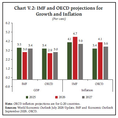 V.2 Inflation Outlook Domestic headline inflation edged up to 4.8 per cent in August, driven primarily by rising food and fuel prices but with increasing evidence of broad-basing of price pressures as evident from diffusion indices (as discussed in Chapter IV). Inflation in food and beverages rose to 5.7 per cent, while core inflation inched up to 4.2 per cent. Going forward, inflation trajectory remains subject to considerable upside risks from overlapping climate and geopolitical shocks. Domestically, outlook is clouded by recent projections from the National Oceanic and Atmospheric Administration (NOAA), USA, warning that the prevailing El Niño phenomenon is set to intensify till the end of 2026 and remain strong in the first half of 2027, posing downside risks to agriculture output, and reservoir replenishment. On the external front, developments in West Asia pose key upside risks, particularly through their impact on global energy prices, commodity markets and supply chains. Renewed geopolitical tensions have kept energy markets volatile and could raise freight, insurance and other transportation costs. Any sustained increase in these costs could feed into domestic retail prices and raise input costs across a range of products, triggering the risk of second-round and broader cost-push pressures. Urban households’ inflation expectations for the next three months as well as one year ahead rose by 70 bps and 60 bps to 9.9 per cent and 10.0 per cent, respectively, in the latest survey round (September 2026) of the Reserve Bank’s bi-monthly households survey.2 The proportion of respondents anticipating a rise in general inflation has inched up for both the time horizons (Chart V.3a). Additionally, according to the Reserve Bank’s recent bi-monthly Rural Consumer Confidence Survey (RCCS)3, the current perception (vis-à-vis a year ago) of inflation in rural and semi-urban households increased by 70 bps to 6.8 per cent in September 2026 as compared with the previous round. Moreover, their one-year ahead expectations also rose by 50 bps to 7.9 per cent. A sequential rise in the inflation expectations has been observed since January 2026 survey round as against the declining trend during the calendar year 2025 (Chart V.3b). 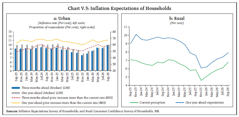 Manufacturing firms surveyed in the July-September 2026 round of the Reserve Bank’s quarterly Industrial Outlook Survey expect pressures from cost of raw materials to persist in Q3:2026-27 with increased pass-through to selling prices (Chart V.4a).4 Services and infrastructure sectors expect some easing of input cost pressures in Q3:2026-27, resulting in moderation in the pace of increase of selling prices (Chart V.4b and V.4c).5 Professional forecasters surveyed by the Reserve Bank in September 2026 projected CPI inflation to increase from 3.9 per cent in Q1:2026-27 to 4.9 per cent in Q2. It is expected to increase further to 5.9 per cent in Q3:2026-27, then moderate to 5.5 per cent in Q4 and further to 4.7 per cent in Q2:2027-28 (Chart V.5a and Table V.3).6 CPI inflation, excluding food and fuel7, is expected at 4.1 per cent during Q2:2026-27, and thereafter remain between 4.3 to 4.7 per cent till Q2:2027-28. Long-run inflation expectations of professional forecasters – measured by their five- and ten-year horizons – is at 4.5 per cent and 4.2 per cent, respectively, in the current round (Chart V.5 b). Considering the initial conditions, signals from forward-looking surveys and estimates from time-series and structural models8, CPI inflation is projected to average 5.2 per cent in 2026-27 with Q2 at 4.9 per cent; Q3 at 6.0 per cent; and Q4 at 5.7 per cent with risks evenly balanced (Chart V.6 and Table V.3). Assuming a normal monsoon, and no further exogenous or policy shocks, structural model estimates indicate that inflation will average 5.0 per cent in 2027-28. The 50 per cent and the 70 per cent confidence intervals for headline inflation in Q4:2027-28 are 3.1-6.1 per cent and 2.3-6.9 per cent, respectively. 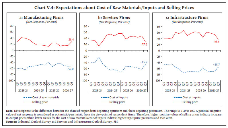
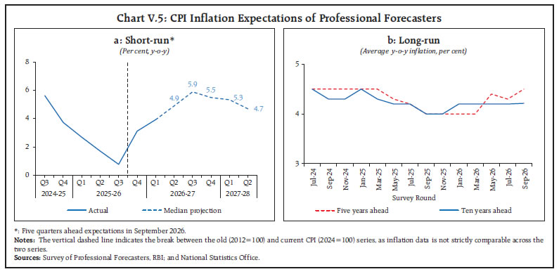
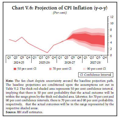
| Table V.3: Projections - Reserve Bank and Professional Forecasters | | (Per cent) | | | 2026-27 | 2027-28 | | Reserve Bank’s Baseline Projections | | | | Inflation | 5.2 | 5.0 | | Real GDP growth | 7.1 | 7.0 | | Median Projections of Professional Forecasters | | | | Inflation, Q4 (y-o-y) | 5.5 | - | | Real GDP growth | 7.1 | 7 | | Gross domestic saving (per cent of GNDI) | 33.2 | 33.5 | | Gross capital formation (per cent of GDP) | 35 | 35 | | Credit growth of scheduled commercial banks | 16 | 13.7 | | Combined gross fiscal deficit (per cent of GDP) | 7.5 | 7.3 | | Central government gross fiscal deficit (per cent of GDP) | 4.5 | 4.3 | | Repo rate (end-period) | 5.75 | - | | Yield on 91-days treasury bills (end-period) | 5.9 | 6.0 | | Yield on 10-year central government securities (end-period) | 7.2 | 7.0 | | Overall balance of payments (US$ billion) | 90 | 10 | | Merchandise exports growth | 11.6 | 4.9 | | Merchandise imports growth | 11.7 | 5.4 | | Current account balance (per cent of GDP) | -1.2 | -1.1 | Note: GNDI: Gross National Disposable Income.
Source: RBI staff estimates; and Survey of Professional Forecasters (September 2026). | The baseline forecasts are subject to both upside and downside risks. Upside risks to inflation are from weather-related shocks as well as a prolonged or renewed escalation of geopolitical tensions that could disrupt energy supplies and global supply chains and keep commodity, freight and insurance costs elevated. Downside risks could emanate from de-escalation of geopolitical tensions and easing of global trade-policy uncertainty, a moderation in global growth and commodity prices, and an improvement in domestic supply conditions, particularly food supplies. V.3 Growth Outlook Domestic economic activity remains resilient supported by private consumption and fixed investment. High-capacity utilisation, robust bank credit growth, conducive financial conditions, and the government’s continued emphasis on infrastructure are expected to stimulate investment activity. Moreover, several measures announced in the Union Budget 2026-27 are also growth supportive. However, spillovers from heightened geopolitical tensions, along with volatility in international financial markets and trade dynamics, pose downside risks to the growth outlook. Forward-looking surveys offer additional insights. The bi-monthly consumer confidence (current situation index) for urban households remained almost at a similar level in September 2026 vis-à-vis the previous round. Consumer confidence of rural households registered a decline in the latest survey round, dipping further into pessimistic zone (Chart V.7). Consumers’ optimism for the year ahead, measured by the future expectations index, remained in positive territory; however, it continued to decline for both urban and rural households in the recent survey round, driven mainly by lower expectations across most survey parameters (Chart V.7).
In the Reserve Bank’s quarterly industrial outlook survey of July-September 2026, manufacturing firms continued to stay optimistic and recorded improved sentiments of the firms from the previous quarter about the business conditions (BAI/BEI)9 (Chart V.8a). The services firms experienced some moderation in sentiments in Q3:2026-27 as compared to previous quarter, while optimism increased for infrastructure firms (Charts V.8b and V.8c). Professional forecasters polled in the September 2026 round of the Reserve Bank’s survey expect real GDP growth to be at 7.2 per cent during Q2:2026-27. Growth is expected at about 6.8-7.1 per cent during the subsequent four quarters (Chart V.9). Taking into account the baseline assumptions, survey indicators and model forecasts, real GDP growth is expected at 7.1 per cent in 2026-27 with 7.2 per cent in Q2; 6.9 per cent in Q3 and 6.8 per cent in Q4 – with risks evenly balanced around this baseline path (Chart V.10 and Table V.3). Assuming a normal monsoon and no major exogenous or policy shocks, structural model estimates for 2027-28 place real GDP growth at 7.0 per cent.
There are upside and downside risks to the baseline growth estimate. Upside risks emanate from easing of geopolitical tensions, abating of trade-related uncertainty and a broad-based revival in private investment. On the downside, spillovers from prolonged geopolitical tensions, volatility in global financial markets, shifting trade patterns, and climate-related shocks pose risks to the baseline growth path. V.4 Balance of Risks The baseline projections of domestic growth and inflation remain conditional on key domestic and global macroeconomic assumptions that are given in Table V.2. These assumptions are subject to evolving uncertainties from ongoing geopolitical tensions in West Asia, commodity price volatility, global trade fragmentation, and domestic weather-related risks. Against this backdrop, this section outlines the balance of risks surrounding the baseline projections under plausible alternative scenarios. (i) Global Growth Uncertainties Global economic activity is navigating crosscurrents from ongoing war-induced supply shocks and a positive technology-led investment cycle. Growth momentum remains highly uneven, with advanced and emerging economies that are integrated into the artificial intelligence (AI) and semiconductor value chains experiencing technology-driven growth. In contrast, activity across energy-importing and non-tech economies are constrained by elevated energy prices, structural headwinds, and trade disruptions. Downside risks to global growth dominate. Broadening geopolitical conflicts in the West Asia may continue to disrupt global supply chains and critical maritime transit routes, particularly the Strait of Hormuz. This continued escalation of geopolitical hostilities may further disrupt the commodity markets. Moreover, elevated policy uncertainty and a potential surge in trade protectionism may restrain international trade flows and investment. High public debt levels in major economies leave sovereign markets exposed to financial tightening, restricting the fiscal space for productive investment. Downside risk also originate from potential sharp downside corrections in AI-related asset valuations which pose contagion risks to global financial markets. On the upside, a durable resolution of geopolitical tensions, swifter normalisation in energy markets, and faster AI-driven productivity gains could lift global growth above the baseline. If global growth turns out to be 100 bps below the baseline, domestic growth and inflation could be lower by around 30 bps and 15 bps, respectively. Conversely, if global growth is higher by 50 bps relative to the baseline, domestic growth and inflation could turn out to be higher by around 15 bps and 7 bps, respectively (Charts V.11a and V.12a). (ii) International Crude Oil Prices Global crude oil markets remain volatile due to supply disruptions in the Gulf region. After prices surged following the onset of the West Asia conflict, brent crude oil scaled a peak of US$105 per barrel in late July 2026 following renewed hostilities and maritime disruptions, before easing to around US$90 per barrel by end August 2026. Prices rose to an average of US$114 during September 2026. According to the Oil Market Report by International Energy Agency (IEA), approximately 10.0 million barrels per day (mb/d) of Gulf output remained unavailable as of August 2026. The IEA projects global oil supply to contract by 5.7 mb/d, while global oil demand is expected to decline by 2.5 mb/d in 2026. The primary upside risks originate from significant supply disruption due to prolonged West Asia conflict, which could threaten major energy infrastructure or further restrict critical maritime transit routes. Additionally, deeper, or prolonged production constraints by major oil-exporting nations, combined with depleted global inventory buffers, could severely tighten supply. If these shocks materialise, a sustained spike in crude oil prices would rapidly transmit to domestic inflation through higher imported fuel costs and second round effects (Box V.1). Assuming full pass-through to domestic product prices, if crude oil prices are higher by 10 per cent than the baseline, inflation could turn out to be higher by around 50 bps and growth may be lower by around 15 bps. Conversely, sharper-than-expected deceleration in global growth, an accelerated resolution to ongoing geopolitical hostilities or robust production increases from non-traditional suppliers could ease prices. If crude oil prices are lower by 10 per cent relative to the baseline, inflation could be lower by around 50 bps and GDP growth could be higher by 15 bps (Charts V.11a and V.12a). Box V.1: Crude Oil Price Shocks: Quantifying the Macroeconomic Impact on the Indian Economy Being an energy importer, crude oil price dynamics remain a critical determinant of macroeconomic stability in India, exerting a profound influence on domestic price stability, external sector balances, and overall growth outlook. Global crude oil prices have experienced extreme volatility in 2026 so far, driven by the West Asian conflict and supply chain disruptions. The Indian crude oil basket spiked to around US$125 per barrel in March 2026. Prices subsequently eased to an average of US$82 per barrel in July, before rising to US$90 per barrel by August 2026. The renewed West Asia conflict has pushed up crude oil prices to $116 per barrel in September 2026. Given India’s heavy reliance on external energy sources, adverse international crude price shocks pose significant pass-through risks to headline inflation – both directly through fuel components and indirectly via generalised cost-push pressures, creating headwinds to medium-term macroeconomic stability. Furthermore, the broader global energy outlook remains clouded by several compounding factors including widespread uncertainty regarding the timeline for supply resumption and the restoration of critical shipping routes. Additionally, global strategic petroleum reserves remain low, leaving markets vulnerable to further shocks. To evaluate how these price fluctuations ripple through the economy, the Quarterly Projection Model (QPM) is utilised to delineate several interconnected channels through which the increase in crude oil prices impacts the economy (John et.al., 2022, 2023). An escalation in crude oil prices adversely impacts key global macroeconomic aggregates, aggravating global inflationary pressures, dampening output growth, possibly triggering higher monetary policy rates. Heightened global energy prices cause import bill to rise, putting downward pressure on the domestic currency, leading to rise in imported inflation. An immediate pass-through of international price movements to domestic energy prices exert an instantaneous upward pressure on headline inflation, capturing the direct effect. The increase in petroleum product prices triggers indirect cost push effects emanating from firms passing on higher input costs, pushing up prices of final goods and services. Concurrently, elevated energy prices compress household real disposable incomes and narrow corporate profit margins, precipitating a contraction in discretionary consumer spending and private investment. This resultant moderation in aggregate demand has a dampening effect on inflationary pressures. 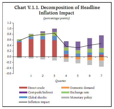 To prevent inflation expectations from getting unhinged, the central bank could raise policy rates. This monetary tightening widens the output gap and compresses demand to bring inflation back to target. Chart V.1.1 depicts the decomposition of impact on headline inflation due to a persistent 10 per cent shock in crude oil prices highlighting the relative strength of the channels of transmission. Higher inflation in the first year is primarily driven by the direct effects, which dissipates over the next year. In the medium term, indirect cost push effects play the prominent role. While the demand channel exerts a moderating impact on price pressures, its offsetting impact is considerably smaller than that of the cost-push channel. Furthermore, monetary policy reaction also imparts a consequential dampening effect on inflation in the medium-term. 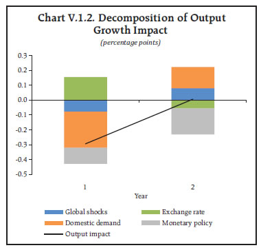 In the case of output growth, the favourable impact of exchange rate depreciation will only be evident in the first year but this impact will be more than offset by moderation in domestic demand as well as weaker global growth. The pass-through of a depreciated currency turns contractionary in the subsequent year, as higher imported costs exert pressure on macroeconomic output (Chart V.1.2). References: John, J., Kumar, D., George, A.T., Mitra, P., Kapur, M. and Patra. M.D. (2023), “A Recalibrated Quarterly Projection Model (QPM 2.0) for India”, Reserve Bank of India Bulletin, February, pp.59-77. John, J., Kumar, D., and Patra, M.D. (2022). Monetary Policy: Confronting Supply-driven Inflation, Reserve Bank of India Bulletin, July, pp. 97-109. | (iii) Exchange Rate The Indian Rupee (INR) was supported by robust FCNR(B) deposit inflows in early September 2026, subsequently, these gains were reversed due to higher crude oil prices. Looking ahead, the INR may face headwinds, including a robust US dollar, elevated import cost, volatile capital inflows and rise in trade policy uncertainties. Any escalation in geopolitical tensions or unexpectedly aggressive monetary tightening by major central banks may put pressure on INR. Conversely, the INR could find support from the resilience of India’s services exports, the stability in bilateral trade frameworks and sustained foreign capital inflows. In a scenario where the INR depreciates by 5 per cent over the baseline, inflation could be higher by around 40 bps, while GDP growth may benefit by around 25 bps through the exports channel in the short term, under normal macroeconomic conditions. In contrast, an appreciation of the INR by 5 per cent relative to the baseline would moderate both inflation and GDP growth by around 40 bps and 25 bps, respectively (Charts V.11b and V.12b). (iv) Food Inflation Domestic headline CPI inflation experienced an uptick in mid-2026, driven primarily by food price pressures. Price pressures across all the classes within the food and beverage basket firmed up. Risk to agricultural crops remain in the wake of deficient and erratic monsoon experienced in 2026-27. Food price risks remain sensitive to weather variations. Adverse impact of El Niño, unseasonal rain, lower reservoir levels, localised heatwaves, higher input costs pose upside risks to food inflation, which may result in headline inflation being higher by 40 bps vis-à-vis the baseline. On the other hand, large buffer stocks, and government's various supply side measures could moderate headline inflation by around 40 bps relative to the baseline (Charts V.11b and V.12b). V.5 Conclusion India’s macroeconomic outlook continues to be supported by resilient domestic economic activity on the back of private consumption and investment. The external environment, however, remains uncertain. At the same time, improving investment outlook, bilateral trade agreements and conducive financial conditions could provide further support to economic activity. On the inflation front, the recent increase in headline inflation has been driven largely by food and fuel prices, but core inflation has also registered a pickup from its benign levels, indicating signs of greater generalisation of price pressures as evident from diffusion indices. Going forward, upside risks to the inflation outlook persist from renewed geopolitical tensions, disruptions to energy supplies and adverse weather conditions. Against this backdrop, potential second-round effects warrant stricter vigilance particularly as demand conditions remain strong. Overall, the outlook for growth and inflation will depend on how domestic demand and supply conditions evolve alongside developments in the global economy, with the balance of risks remaining contingent on these factors. _________________________________________________________________________________
ABBREVIATIONS | A | Actuals | | AEs | Advanced Economies | | AI | Artificial Intelligence | | bbl | Barrel | | BE | Budget Estimates | | BoP | Balance of Payment | | bps | Basis Points | | CAG | Comptroller and Auditor General of India | | CAGR | Compounded Annual Growth Rate | | CCIL | Clearing Corporation of India Limited | | CD | Certificate of Deposit | | CEIC | China Economic Information Centre | | CMIE | Centre for Monitoring Indian Economy | | CNG | Compressed Natural Gas | | CPB | Central Plan Bureau | | CPI | Consumer Price Index | | CPs | Commercial Papers | | CRR | Cash Reserve Ratio | | CU | Capacity Utilisation | | DGCI&S | Directorate General of Commercial Intelligence and Statistics | | EBLR | External Benchmark-based Lending Rate | | ECB | External Commercial Borrowing | | EM | Emerging Market | | EMEs | Emerging Market Economies | | FAO | Food and Agriculture Organization of the United Nations | | FAR | Fully Accessible Route | | FBIL | Financial Benchmarks India Pvt. Ltd. | | FCNR(B) | Foreign Currency Non-Resident (Bank) | | FDI | Foreign Direct Investment | | Fed | Federal Reserve | | FMCG | Fast Moving Consumer Goods | | FPI | Foreign Portfolio Investment | | FPIs | Foreign Portfolio Investors | | FPO | Follow on Public Offer | | F-TRAC | FIMMDA Trade Reporting and Confirmation System | | G7 | Group of Seven comprising Canada, France, Germany, Italy, Japan, UK and US | | GDP | Gross Domestic Product | | GFCF | Gross Fixed Capital Formation | | G-Secs | Government Securities | | GST | Goods and Services Tax | | GVA | Gross Value Added | | HFCs | Housing Finance Companies | | HSBC | Hong Kong and Shanghai Banking Corporation | | ICRIER | Indian Council for Research on International Economic Relations | | IIP | Index of Industrial Production | | IMD | India Meteorological Department | | IMF | International Monetary Fund | | INR | Indian Rupee | | IPO | Initial Public Offer | | IRDAI | Insurance Regulatory and Development Authority of India | | IT | Information Technology | | LAF | Liquidity Adjustment Facility | | LPA | Long Period Average | | LPG | Liquefied Petroleum Gas | | MCLR | Marginal Cost of funds-based Lending Rate | | MGNREGA | Mahatma Gandhi National Rural Employment Guarantee Act | | MoSPI | Ministry of Statistics and Programme Implementation | | MPC | Monetary Policy Committee | | MPR | Monetary Policy Report | | MSCI | Morgan Stanley Capital International | | MSME | Micro, Small and Medium Enterprises | | NBFCs | Non-Banking Financial Companies | | NDTL | Net Demand and Time Liabilities | | NSO | National Statistics Office | | OECD | Organisation for Economic Co-operation and Development | | OMOs | Open Market Operations | | PA | Provisional Accounts | | PE ratio | Price to Earnings Ratio | | PIB | Press Information Bureau | | PLFS | Periodic Labour Force Survey | | PMI | Purchasing Managers’ Index | | POL | Petroleum, Oil & Lubricants | | PPAC | Petroleum Planning & Analysis Cell | | PSBs | Public Sector Banks | | PSUs | Public Sector Undertakings | | PVBs | Private Banks | | QMA | Quarter Moving Average | | RBI | Reserve Bank of India | | RE | Revised Estimate | | RECO | Revenue Expenditure to Capital Outlay Ratio | | REER | Real Effective Exchange Rate | | RHS | Right Hand Side | | S&P | Standard and Poor’s | | SAAR | Seasonally Adjusted Annualised Rate | | SAE | Second Advance Estimates | | SCBs | Scheduled Commercial Banks | | SDF | Standing Deposit Facility | | SLR | Statutory Liquidity Ratio | | T-Bill | Treasury Bill | | TOP | Tomato, Onion, and Potato | | UK | United Kingdom | | US | United States | | USD | US Dollar | | UT | Union Territory | | VAR | Vector Auto Regression | | VRR | Variable Rate Repo | | VRRR | Variable Rate Reverse Repo | | WACR | Weighted Average Call Rate | | WADR | Weighted Average Discount Rate | | WADTDR | Weighted Average Domestic Term Deposit Rate | | WALR | Weighted Average Lending Rate | | WPI | Wholesale Price Index | | WTO | World Trade Organisation | |