Snehal S. Herwadkar, Shubham Gupta and Vaishnavi Chavan* Received on: June 17, 2022
Accepted on: December 07, 2022 In recent years, the Indian banking sector has witnessed hectic activity in the merger space. Compiling data on bank mergers since 1997, the paper analyses the impact of bank mergers on the short-term and medium-term performance of the acquirer banks. Data envelopment analysis (DEA) suggests that the efficiency of acquirers improved post-merger due to an increase in scale or productive capacity. Financial ratio analysis, which compares the pre- and post-merger performance of acquirers, reinforces the findings of efficiency analysis. These results are robust even after controlling for industry-wide impact. The event study analysis employed for bank mergers between 2019 – 2020 indicates an increase in shareholders’ wealth of the acquiree banks. The study identifies geographical diversification and greater focus on interest earnings as a source of income as the key factors behind post-merger improvement in bank efficiency. JEL Classification: C61, G21, G34 Keywords: Bank mergers, M&As, efficiency, financial ratios, DEA, Tobit model, event study Introduction In the recent years, the Indian banking sector has witnessed a flurry of activity in the merger space. In one of the biggest consolidations of the sector, ten public sector banks (PSBs) were merged into four, effective April 1, 2020. The Government of India while announcing the merger plan suggested that, “The adoption of best practices across amalgamating entities would enable the banks improve their cost efficiency and risk management…” (PIB, 2019). More than two years have elapsed since the mega-merger and the impact assessment in the literature appears to be divided. While certain studies suggest that non-performing assets (NPAs) of weak merging banks declined by 10 per cent, almost entirely due to a decline in strategic defaults (Kashyap et al., 2022), some researchers, on the other hand, argue that, “the merger decisions were not necessarily on efficiency grounds, and hence, post-merger benefits are minimal” (Das and Kumbhakar, 2022). The aim of the present paper is to analytically evaluate the impact of mergers on the acquirer banks. The expected benefits of mergers and acquisitions (M&As) in financial institutions worldwide, including in India, are cost reduction, profit maximisation, and gains through portfolio or geographical diversification. Mergers impact shareholders’ wealth, alter capital infusion requirements in case of weak banks, and can also lead to reduced competition and creation of too-big- to-fail (TBTF) banks that may have a systemic impact. Historically, M&As in banks are aimed at improving financial performance and efficiency, either by resolving the problem of distressed banks or by ameliorating economies of scale.1 For example, most of the European bank mergers in the 1990s were either for defensive purpose of inefficient acquired entity or for improving their competitiveness in the European Union (Azofra et al., 2008). Evidence from the US banks suggests that mergers strengthened the credit market by allowing banks to achieve higher economies of scale while minimising their costs (Al-Sharkas, 2008). In the emerging market economies (EMEs) as well, bank mergers were undertaken primarily for revenue maximisation and cost reduction (Berger et al., 1998). Higher scale efficiency is documented to be one of the major causes behind mergers of South African banks post global financial crisis (Wanke, 2017). Protecting distressed banks was a key motivation behind EME bank mergers, especially those led by government policy (Sufian, 2007; Joshua, 2011). However, economic literature so far is not unanimous on “….whether the participating banks indeed benefit from M&As, whether their customers share the benefits, or whether systemic risks increase or decrease after the merger…” (DeYoung et al., 2009). Globally, previous studies have employed performance ratio approach, efficiency analysis and event studies to evaluate the benefits of bank M&As. Contemplating bank mergers since 1997, for both public and private sector banks, the current study employs all the three approaches used in the literature to gauge whether bank mergers in India resulted in short-term and medium-term gains for the acquirer banks. The paper also attempts a deep dive into factors contributing to efficiency gains. In particular, the paper seeks to answer four questions: a) What were the efficiency characteristics of acquirer and acquiree banks pre-merger? In particular, whether the mergers were amongst equals or between a strong and a weak bank?; b) Whether the financial performance and efficiency of acquirers improved or deteriorated post-merger? And what contributed to the efficiency gains post-merger—gains in managerial prowess or scale efficiencies?; c) Did geographical diversification or changes in the source of income (greater focus on interest earnings as compared to non-interest earnings) had a role to play in efficiency improvement?; and d) How did the recent mergers perform, especially with reference to their impact on shareholders’ wealth. Our findings, using the non-parametric technique of data envelopment analysis (DEA) suggest that mergers, on an average, improved the efficiency of acquirers—both in the short-term (1 year and 3 years since merger) and medium-term (5 years since merger). A more nuanced analysis suggests that this improvement was due to increased scale of productive capacity (scale efficiency). These findings are supported by financial ratio approach, where the pre-merger financial performance of acquirers is compared to that in the post-merger period. Additionally, the results remain robust when compared to the average performance of the ‘control group’—consisting of all scheduled commercial banks (SCBs). The event study approach employed for mergers during 2019-2020, where adequate data is still not available, suggests that mergers resulted in an increase in shareholders’ wealth of the acquiree banks, while the share price of acquirer banks witnessed a temporary blip. Furthermore, the paper makes an innovative contribution to the existing literature by analysing factors that may have contributed to efficiency gains. Using Herfindahl-Hirschman index (HHI) as a measure of geographical concentration, the paper finds that mergers have led to higher geographical diversification for acquirers. Results of panel Tobit regression analysis suggest that geographical diversification coupled with changes in earning sources—away from non-interest income to interest income—resulted in post-merger improvement in bank efficiency. The rest of the paper is structured as follows: Section II reviews the relevant literature. Section III presents an overview of bank M&As in the Indian context. Section IV gives a detailed description of the data and methodology used. Section V is devoted to empirical findings and analysis of results. Section VI concludes the study. Section II
Literature Review The literature on bank M&As is vast and can be largely divided into four strands. Studies that focus on the impact of M&As on the financial performance of banks employ the performance analysis using accounting ratios, efficiency frontier analysis using either DEA or stochastic frontier analysis (SFA), and/or event study analysis (Kolaric and Schiereck, 2014). Another strand of literature focuses on the non-financial motives behind mergers. These include ‘fringe utilities’ like enhanced managerial power of the CEO and the financial benefits of becoming a ‘too-big-to-fail (TBTF)’ institution. Studies have also evaluated the benefits accrued due to various types of diversification—across financial products and across geographies—as a fallout of mergers. Lastly, some studies are devoted to documenting the benefits received by borrowers, depositors, and external stakeholders due to mergers. The event study is another commonly used technique of impact assessment for banking M&As. This method involves investigating the publicly traded stock returns of the acquirer and acquiree banks around the merger announcement date. Specifically, abnormal/expected stock returns are estimated, and a merger is considered successful if the actual stock returns received by the investors exceed the abnormal returns. In the bank M&As literature, most event study analysis suggest a positive and statistically significant abnormal stock returns for the acquiree banks and negative returns for the acquirers (Hannan and Wolken, 1989; Cornett and Tehranian, 1992; Houston and Ryngaert, 1997; DeLong, 2003a; Campa and Hernando, 2006; Al-Sharkas and Hassan, 2010). However, recent studies for the US, Euro and EMEs report non-negative returns for the acquirers also (Kolaric and Schiereck, 2014). Kiymaz (2004, 2013) reports that the US banks involved in cross-border M&A transactions generated positive abnormal returns for the acquirer and acquiree banks. Kolaric and Schiereck (2013) and Goddard et al. (2012) find positive abnormal stock returns for Asian and Latin American bank mergers over a long-term period. Similarly, Ismail and Davidson (2005, 2007) report positive abnormal stock returns for both the parties involved in the merger transaction for European banks. As per Houston et al. (2001), better valuation of bank M&A transactions or better access to information for the acquirers may have attributed to positive abnormal returns for the acquirer banks. Similar to the results from developed economies, evidence from EMEs showed mixed or no significant impact of mergers on cumulative abnormal returns (CARs)2 to the shareholders of acquirer banks. Evidence from the Middle East and North African region showed that mergers did not have significant positive or negative impact on shareholders’ wealth (Sindi et al., 2018). The study on Indian banking mergers found a mixed impact of the announcement of bank mergers—merger announcements had limited impact on the volatility of share prices and no significant impact on the liquidity of the shares of acquirers (Kumar et al., 2013). Since the merger news is often leaked in the market much before the official announcement day, researchers have also used ‘date of leakage’ i.e., the date on which the news of the merger first reached the market instead of the official announcement date (Houston and Ryngaert, 1994, 1997; Houston et al., 2001), while others have simply extended the event window to account for the information leakage (Amihud et al., 2002). In the case of performance studies using accounting ratios, pre- and post-merger financial health parameters like capital adequacy, profitability, operational efficiency, liquidity, asset quality, loan loss provisions, etc. are compared. A merger is considered successful if the combined entity’s financial performance improves post-merger. The empirical evidence from the studies using accounting ratios to ascertain the success/failure of bank M&As is heterogeneous. In the US, performance studies have obtained both positive (Boyd and Graham, 1988; Cornett et al., 2006) and negative (Linder and Crane,1993; Knapp et al., 2005) results from bank M&As. Similarly, results from performance studies for European banking M&As are also mixed and highly sensitive to the period under investigation (Kondova and Burghof, 2007). Reda (2013) showed that profitability and liquidity ratios for Egyptian banks deteriorated post-merger, however, there was a significant improvement in their risk management practices. In the Indian context, Bishnoi and Devi (2015) did not find any significant improvement in performance indicators of acquirer banks post-merger. A few studies also use a control/peer group to account for the noise not directly related to merger-related sources. Kwan and Wilcox (1999) show that for the US bank mergers between 1985 and 1997, the operating expenses (both labour cost and occupancy expense) of the merged entities reduced significantly compared to their non-merging peers. Other studies simply exclude the merger year to account for the distortion in cost performance due to differing accounting methods (Linder and Crane, 1993; Cornett et al., 2006). Efficiency analysis for bank M&As, on the other hand, employs frontier analysis using accounting data to estimate a cost or profit function of the best performing bank in the sample, to which other banks are compared. The closer a bank gets to the efficiency frontier after the merger, the higher is the improvement in its efficiency. Parametric techniques like the SFA and non-parametric techniques like DEA are used to estimate efficiency (Liu and Tripe, 2003). However, non-parametric techniques are preferred as they avoid the complexities arising out of assuming a specific functional form i.e., distributional assumptions about the explained/error terms, restriction for minimum sample size, etc. Worldwide evidence on whether bank mergers lead to efficiency gains is mixed, both in the developed and EMEs. In a study of 57 US bank mergers between 1981–1989, Akhavein et al. (1997) found that mergers led to improvement in profit efficiency of the acquiring banks. Similar results were observed for the UK bank mergers between 1981–1993 (Haynes and Thompson, 1999). Al-Sharkas et al. (2008) show that the US bank mergers between 1985–1999 improved both cost and profit efficiency of the acquirer banks. On the other hand, Fixler and Zieschang (1993) reported deterioration in cost efficiency of the US banks that underwent M&As in 1986. Overall, a majority of efficiency studies on the US bank mergers report mixed results (Rhoades, 1998; DeYoung, 1997; Fried et al., 1999; Peristiani, 1997). Comparing pre- and post-merger DEA efficiency scores of Australian trading banks, Avkiran (1999) concluded that before merger, acquirer banks were more efficient than their acquirees and in-market mergers resulted in increased efficiency post-merger. Similarly, evidence for bank mergers between 1989-1998 in New Zealand suggested improvement in employee productivity and post-merger efficiency gains in five out of six banks (Liu and Tripe, 2003). Echoing these findings for Egypt, Reda (2013) documented significant improvement in managerial efficiency of banks post-merger. In a study of seven bank mergers in Malaysia during 2000, Sufian (2007) suggested that the technical efficiency of the acquirer banks improved post-merger. Sufian and Majid (2009) also show that Singaporean banks became relatively more scale inefficient after mergers. In Taiwanese banking sector, scale efficiency of acquirers improved post-merger due to portfolio diversification and therefore, Lee et al. (2013) suggested multi-product strategy to lower production costs. In the Indian banking sector, evidence proposed by Jayaraman et al. (2014) suggests that the technical efficiency of merged banks deteriorated in immediate periods post-merger but improved in the third year since merger. However, mergers did not have significant impact on profitability and cost efficiency. In contrast, the findings of Singh (2009) suggested that bank mergers post-2000 did not have any adverse impact on profit and cost efficiency of acquiring banks and short-term losses were recovered quickly. Das and Kumbhakar (2022) suggested that the recent wave of mergers in India had only limited efficiency gains. Niche segment of regional rural banks (RRBs) were also documented to achieve remarkable improvement in post-merger technical efficiency, pure technical efficiency as well as scale efficiency (Antil et al., 2020). Nishat (2020) found that although scale efficiency of Indian PSBs did not change significantly post-merger, their managerial efficiency improved significantly due to better planning and managing techniques. Overall, the empirical evidence of impact of bank M&As has been mixed across all the three prominent methodologies. Each methodology has its own distinctive pros and cons while assessing a merger transaction. Event study analysis is best suited when the ultimate goal of the analysis is to focus on shareholders’ wealth creation. However, the market assessment of the merger deal may be erroneous around the merger announcement date which makes interpreting short-term success as an indication of long-term success questionable (Kolaric and Schiereck, 2013). Efficiency and performance studies, on the other hand, are more useful to investigate the medium to long-term effects of M&As. Section III
M&As in the Indian Banking Industry Analogous to other EMEs, bank mergers in India were government policy driven during the nationalisation phase (1960 to 1969), when distressed banks were consolidated with stronger banks. Subsequently, however, there was a relative lull in the merger activity till the economy embarked on the liberalisation process (Table 1). The intellectual rationale for bank mergers in the post-liberalisation period was provided by the Narasimhan Committee Reports (1991, 1998)—that recommended banking consolidation, both in the public and private sectors and even with financial institutions and NBFCs—to make them stronger and more competitive. | Table 1: Bank M&As in India | | Period | Number of Mergers | | Pre-nationalisation of banks (1961-1968) | 46 | | Nationalisation to Liberalisation period (1969-1996) | 14 | | Post-Liberalisation period (1997-2022) | 40 | | Total | 100 | | Sources: RBI, 2008; and STRBI, various issues. | In contrast to the nationalisation phase, the consolidation during the post-liberalisation phase was primarily market-driven with an objective to enhance efficiency and gain greater resilience. During 1997-2022, there were 40 bank amalgamations, out of which 12 were between private sector banks (PVBs) and PSBs, 16 were amongst PSBs and the remaining 12 were between PVBs and foreign banks. The consolidation of State Bank of India (SBI) with its associates (during 2008-2017) and the mega merger of ten banks into four in April 2020 account for majority of PSB mergers. Further, bank amalgamations prior to 1999 were primarily triggered by weak financial conditions of the acquiree banks whereas post-1999, business and commercial considerations (such as, the need for increasing market share, operational synergies, acquisition of a business unit or segment, etc.) have also influenced mergers between healthy banks (Leeladhar, 2008). Section IV
Data and Methodology The study covers all registered M&As in the Indian commercial banking industry between 1997 to 2020. The following criteria was used for a merger to be considered under the study: (a) consistent data availability in line with the research design; (b) both the acquirer and the acquiree bank should either belong to public sector (PSB) or private sector (PVB) bank-group3, and (c) a single merger application within the period of analysis, although there could be multiple acquiree banks during the same merger year. In cases with multiple mergers in consecutive years, the latest merger application was considered4, and a single merger observation was considered for cases where multiple acquiree banks were merged with an acquirer in the same year.5 After applying these criteria, the sample reduced to 17 merger cases during 1997-2017 (Annex I) and five merger cases during 2019-2020 (Annex II). Table 2 illustrates the descriptive statistics of the acquiree and acquirer banks involved in M&As during 1997-2017. Bank-level financial data from 1994 to 2022 was compiled from audited financial statements of banks and Statistical Tables Relating to Banks in India (STRBI) published by the Reserve Bank of India (RBI). Apart from acquiree and acquirer banks, data was also collated for all the remaining PVBs and PSBs operating in India, as the latter group formed the ‘control group’ for statistical analysis. | Table 2: Data Description6 | | (₹ crore) | | Bank Type | Summary Statistics | Net Loans & Advances | Investments | Total Assets | Deposits | Capital Reserves & Surplus | Operating Profit | | Acquiree Banks | Average | 28,881 | 11,256 | 45,667 | 34,320 | 7,137 | 754 | | SD | 93,410 | 33,338 | 142,963 | 105,210 | 26,007 | 2,526 | | Median | 1,665 | 1,713 | 4,444 | 3,631 | 244 | 46 | | Min | 15 | 10 | 43 | 36 | 5 | (273) | | Max | 389,474 | 139,578 | 597,138 | 440,227 | 107,847 | 10,479 | | Acquirer Banks | Average | 176,982 | 80,606 | 300,490 | 218,677 | 20,501 | 5,575 | | SD | 362,127 | 145,635 | 587,441 | 434,379 | 36,441 | 10,834 | | Median | 34,756 | 25,055 | 72,915 | 53,986 | 3,381 | 1,347 | | Min | 2,110 | 2,861 | 6,982 | 6,073 | 308 | 82 | | Max | 1,463,700 | 575,652 | 2,357,618 | 1,730,722 | 144,274 | 43,258 | Note: Data pertains to end-March of the year prior to the M&A year.
Source: STRBI, Authors’ calculations. | To measure the impact of merger, comparing data of up to three years prior to the merger event with that up to three years afterwards is the most common practice in the literature (Rhoades, 1998; Avkiran, 2006; Liu and Tripe, 2003; Sufian and Majid, 2009; Bishnoi and Devi, 2015). Most researchers have argued that the performance of banks might deteriorate in the immediate years following merger due to organisational changes, but a minimum of three-year window is required to absorb the effects and to reflect its impact on managerial and scale efficiency (DeYoung et al., 2009; Berger et al., 1998). On the other hand, any time window beyond 5 years will be too long, where apart from factors relating to mergers, influence of other factors may dominate. Motivated by earlier literature, the study analyses the impact of M&As on the financial performance and efficiency of the merged entities in short term i.e., (-1, +1) years, (-3, +3) years and the medium-term (-3, +5) years. A. Financial Ratio Analysis Financial ratios are the health indicators of banking institutions. The current study computes mean financial ratios of the banks involved in M&As over three years before merger to see if the acquirers had better financial health than their acquirees. The study also compares the mean financial ratios of the acquirers over the short-term —(- 1, +1), (-3, +3) and the medium-term (-3, +5) event window, excluding the merger year to see if the financial conditions of the acquirers improved post-merger. Following Reda (2013) and Cornett et al. (1992), the study looks at 15 financial ratios, covering liquidity, profitability, operating efficiency, capital adequacy, asset quality and NPA provisions aspects that have implications for revenue enhancement, cost cutting and solvency of the banks. Detailed definitions for each are provided in Annex III. Although financial ratio analysis is the most rudimentary and widely used approach to investigate the effects of banking M&As, it has certain limitations. One of the major drawbacks is that it relates only one input to one output at a time (Chen and Ali, 2002). Banks typically use multiple inputs to produce one or more outputs, with no one-to-one correspondence. A performance metric based on the ratio of a single output to a single input fall short of capturing the comprehensive view of their performance. To avoid this, literature suggests that the ratio analysis may be complemented with other approaches, such as the frontier approach (Thanassoulis et al., 1996). In this vein, the present study also explores the non-parametric DEA frontier approach to analyse the impact of banking M&As in the Indian context. B. Data Envelopment Analysis In the recent years, researchers have increasingly used efficiency measures—such as DEA and SFA to gauge the impact of M&As. SFA requires a parametric specification for the efficient frontier and its statistical noise (Anwar, 2011). In contrast, the non-parametric approaches such as DEA—developed by Charnes, Cooper and Rhodes (CCR) in 1978—avoids the complexities arising out of assuming a specific functional form (i.e., distributional assumptions about the explained/error terms, restriction for minimum sample size, etc.). Moreover, for banking services, DEA is a more suitable approach as it helps in simultaneously modelling multiple outputs for a given set of inputs and allows researchers to choose a combination of inputs and outputs, regardless of different measurement units (Avkiran, 2006). DEA uses linear programing methods to construct a ‘grand frontier’ based on a piecewise linear connection of the best-practice decision making units’ (DMUs) efficiency scores, to which other DMUs in the sample are compared, to obtain relative efficiency scores. In essence, it estimates relative efficiency scores by maximising the ratio of weighted outputs to weighted inputs and a DMU is said to have become efficient if it moves closer to the grand frontier (refer to Annex IV for details). The relative efficiency of each DMU lies between 0-100, where an efficiency score of 100 implies that the DMU is situated at the best-practice frontier. On the other hand, an efficiency score of less than 100 implies that the DMU is relatively inefficient than the best-practice DMU and imply sub-optimal behaviour. Thus, the advantage of using DEA approach is that it also highlights the areas that need improvement for each DMU (Sufian and Majid, 2009). DEA model developed by CCR in 1978 estimates the overall technical efficiency (TE) scores of input-output transformations under the assumption of constant returns to scale (CRS). Later, in 1984, Bankers, Charnes and Cooper (BCC) extended the CCR model to include variable returns to scale (VRS) which provides estimates for pure technical efficiency (PTE) devoid of scale effects. The scale efficiency (SE) is computed as the ratio of technical efficiency to pure technical efficiency, i.e., SE = TE/PTE This paper employs the output-oriented7 DEA with CRS to compute TE of acquiree and acquirer banks involved in M&As and then decomposes the TE into two mutually exhaustive components – PTE and SE to identify the sources of efficiency (inefficiency) post-merger. In essence, PTE measures the controllable, managerial or overall organisational efficiency in transforming a DMU’s inputs into outputs whereas SE captures the efficiency of a DMU attributable to its size and production level. A scale efficient firm will produce where production frontier exhibits CRS (Alexander and Jaforullah, 2005; Sufian, 2007; Reda, 2013). Choice of Production Approach The choice of appropriate inputs and outputs for measuring banking efficiency remains a contentious issue among researchers. As majority of banking services are jointly produced where the costs/revenues are jointly assigned to a bundle of financial products, it is difficult to classify inputs and outputs separately (Antil et al., 2020). Nevertheless, two main approaches to model bank production dominate the literature: production approach and intermediation approach (Sealey and Lindley, 1977). Under the production approach—pioneered by Benston (1965)—output is measured as the number of accounts rather than the rupee value of services provided and costs include all operating expenses, except the interest paid on deposits (as deposits are considered as output). This approach focuses on the operational aspect of banking business and is more appropriate for measuring branch-level efficiency (Berger and Humphrey, 1997). The intermediation approach (also known as the asset approach), on the other hand, considers banks as financial intermediaries between savers and borrowers that purchase labour, physical capital (fixed assets and equipment), deposits and other liabilities to produce interest-earning assets such as loans and advances, investments and other securities (Sealey and Lindley, 1977). Unlike the production approach, outputs are measured as the rupee value of assets and this approach is well suited for bank-level efficiency studies. Moreover, this approach includes interest expense (which constitute a large proportion of a bank’s total cost) along with operational expenses (Mester, 1987). Following several previous studies (Charnes et al., 1990; Bhattacharyya et al., 1997; Avkiran, 2006; Sathye, 2001; Isik, 2002; Liu and Tripe, 2003; Sufian and Majid, 2009), the current paper also uses the intermediation approach for measuring banking efficiency. Choice of Inputs and Outputs for Bank Production In DEA, a limited number of variables are employed to avoid the issue of over-specification of the model. Moreover, using a large number of variables may inflate the efficiency scores and in case of very small samples, this may lead to all DMUs being on the efficient frontier. On the other hand, omission of relevant variables can lead to underestimation of efficiency with the effect being amplified in case of irrelevant variables in the DEA model. Thus, the current study uses a limited number of inputs and outputs which satisfy the rule of thumb specified by Cooper et al. (2002).8 Although the choice of inputs-outputs in a DEA model is left to the user’s discretion, judgement, and expertise (Nataraja and Johnson, 2011), the selection of inputs and outputs in the current study is guided by the availability of data and previous studies. As per Avkiran (1999), potential inputs under the intermediation approach include deposits, interest expense, non-interest expense, number of employees (full time equivalent), other purchased capital, physical capital (fixed assets and equipment), demographics and competition. Potential outputs include net interest income, non-interest income, consumer loans, housing loans, commercial loans and investments. Given that DEA is sensitive to the choice of input-output mix, this study explores four DEA models (Table 3) such that the above-mentioned rule of thumb is satisfied for all four models. | Table 3: DEA Model Specification | | | Model 1 | Model 2 | Model 3 | Model 4 | | Inputs | 1. Non-Interest Expense
2. Interest Expense | 1. Non-Interest Expense
2. Interest Expense | 1. Non-Interest Expense
2. Interest Expense | 1. Non-Interest Expense
2. Deposits
3. Borrowings | | Outputs | 1. Non-Interest Income
2. Net-Interest Income | 1. Investments
2. Total Loans | 1. Non-Interest Income
2. Net-Interest Income
3. Total Loans
4. Investments | 1. Operating Income
2. Total Loans
3. Investments | In line with the past research (Avkiran, 2006; Sathye, 2003; Kao and Lui, 2004; Sufian, 2007; Reda, 2013; Sonai et al., 2020), interest and non-interest expense are used as the input variables in the first three models. These inputs are used to generate interest and non-interest income—the outputs in Model 1. Alternately, these inputs also help generate investments and total loans—the outputs in Model 2. Model 3 combines the input-output mix of the earlier two models and Model 4 uses a different set of input-output combination that account for a larger proportion of the intermediation function of banking business (Liu and Tripe, 2003). Here, deposits include domestic and foreign demand, savings and term deposits of customers and other banks and borrowings comprise of borrowings from the central bank (RBI), other banks and agencies. Since DEA efficiency scores change with the change in inputs and outputs, average efficiency scores across these four models are used as robust estimates of banking efficiency. C. Tobit Regression Given that the efficiency scores are bounded within [0,100], the study uses panel data Tobit model to investigate the factors that could have led to efficiency improvement for the acquirer post-merger. The Tobit regression for panel data with individual specific effects has the following specification:
D. Event Study Following (MacKinlay, 1997; Mathur et al., 2021), we employ an event study model to evaluate bank mergers during 2019-2020. Under this approach, the change in shareholders’ wealth or abnormal return—the stock return in excess of the expected return is calculated using the market model as: The calculated ARs are indexed to 0 on day (-1) of the event window and cumulated over the next days to obtain the cumulative abnormal returns (CARs). The average CARs for all bank in the sample over each day of the event window are plotted, using bootstrap 95 per cent confidence intervals. Section V
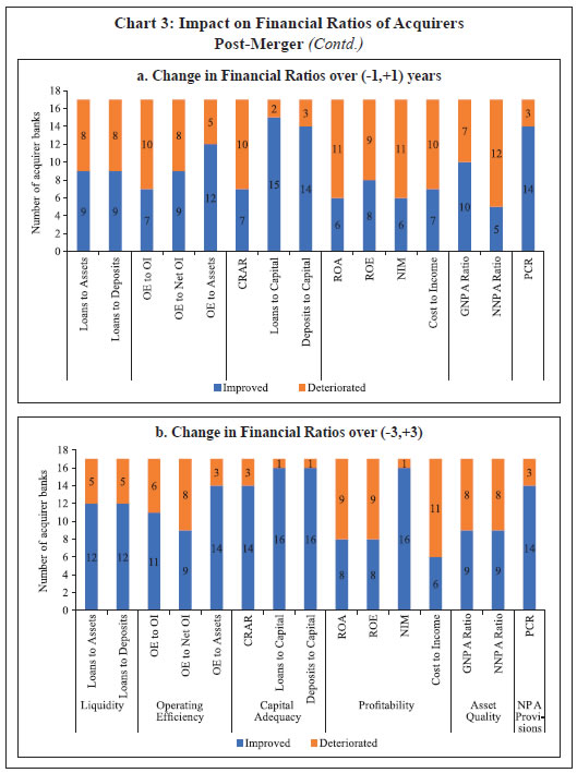
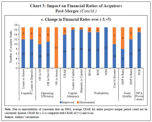
Empirical Results The empirical analysis of the paper can be broadly divided into two parts. In the first part, using data on bank M&As during 1997-2017, we evaluate three questions: (a) were the acquirers more financially sound and efficient than their acquirees before the merger i.e., over (-3,0) years event window; (b) whether the efficiency of acquirers improved or deteriorated post-merger over the short-term — (-1, +1), (-3, +3) years and medium-term (-3, +5) years event window. Both these questions are evaluated using financial ratio analysis as well as DEA. The study also explores if changes in efficiency scores post-merger were due to changes in scale efficiency or pure technical efficiency—evaluated through the decomposition of overall TE scores into PTE and SE; and (c) whether geographical diversification and/or changes in source of income (greater focus on interest earnings as compared to non-interest earnings) were responsible for efficiency changes post-merger—evaluated using panel Tobit regression analysis. The second part is devoted to the analysis of bank mergers during 2019-2020 using event study analysis, as post-merger longer time series financial data in line with the current research design is still not available. However, we have extended the financial ratio analysis as well as the efficiency analysis for as much time period as possible. V.1 Were the acquirers more efficient than their acquirees, pre-merger? Theoretically, a financially sound and more efficient bank should acquire a weak and inefficient bank as that would lead to an increase in the overall efficiency of the banking system (Avkiran, 2006). The findings of some studies in the Indian context, however, suggest that government-led mergers were aimed at accommodating less efficient banks, which did not improve the overall efficiency (Das and Kumbhakar, 2022). Using bank mergers during 1997-2017, we analyse the question in the Indian context. Using the financial ratio analysis, we find that acquirers, across all the metrics, on an average, had better financial health as compared to their acquirees in the pre-merger period (Chart 1). To extend the analysis through DEA, we compare the pre-merger (i.e., three years before the merger year) mean11 TE scores of acquirers to that of their acquirees. In most cases, the acquirers were found to be more efficient than their acquirees in the pre-merger period (Chart 2). On an average, acquirers were 4 per cent more technically efficient than acquirees in the pre-merger period. Parametric (t-test and bootstrap t-test) and non-parametric (Mann-Whitney [Wilcoxon Rank-Sum]) test results confirm the findings that the mean difference between acquirers’ and acquirees’ TE is statistically significant (Table 4). Presumably, most of the mergers amongst PVBs were market-driven and those between PSBs were government-led mergers. Our analysis suggests that the efficiency trends between acquirers and their acquirees were consistent across ownership patterns. Therefore, signalling out the government-led mergers alone as being aimed at accommodating weak banks with stronger ones may not be correct. V.2 Did the acquirers perform better post-merger? Financial ratio analysis suggests that while mergers led to improvement in acquirers’ efficiency across most of the metrics, it was most prominent for liquidity, capital adequacy, profitability and NPA provisions measures. Moreover, the impact was sharper in the medium term (-3 to +5 years period) as compared to the short-term (-1 to +1 years or -3 to +3 years period) (Chart 3). Gains in liquidity indicators suggest that post-merger, the intermediation function of the combined entity improved—banks were able to channelise higher share of deposits/assets into loans. The improvement in capital adequacy and NPA provisions measures indicate that post-merger, the combined entity has become relatively more resilient to financial risks. The improvement in profitability ratios may be indicative of economies of scale—post-merger, banks may have been able to cut some operating costs by consolidating bank branches/ATMs operating in the same area, etc. These gains were also complemented by improvement in operating efficiency as well as asset quality indicators. | Table 4: Acquirer vs Acquiree Mean TE Pre-Merger | | Individual Tests | Test groups | | Parametric Test | Non-Parametric Test | | T-test | Bootstrap t-test | Mann- Whitney [Wilcoxon Rank-Sum] test | | Hypothesis | P(T ≤ t) | P(T ≤ t) | P(Z ≤ z) | | Test Statistics | Mean | t | Mean | t | Mean rank | z | | Pre-Merger (-3,0) | | | | | | | | Acquiree | 86.29 | -2.233** | 86.29 | -2.263** | 13.94 | -2.084** | | Acquirer | 90.88 | | 90.88 | | 21.06 | |
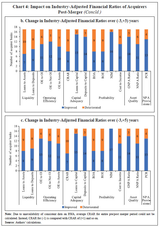
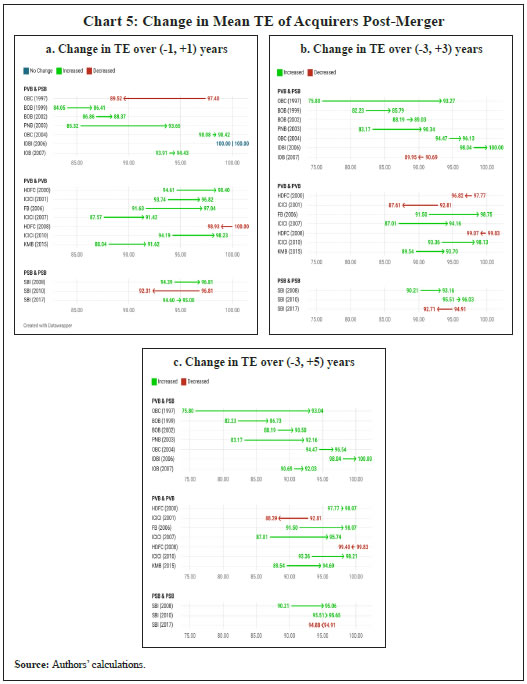
 One drawback of comparing the post-merger financial ratios of the acquirer with its own pre-merger ratios is that such a comparison ignores changing macroeconomic circumstances. For example, it could be argued that during the three/ five-year period under consideration, the credit cycle may have turned, thus making all the banks more profitable and the merger may not have had a significant role to play. In order to address this issue, comparison of the acquirer with industry average performance is suggested in the literature (DeLong, 2003b). Following this method, we calculate how far the financial ratios of acquirers were in comparison to the industry average, pre-and post-merger. The findings of this exercise corroborate the earlier findings—across most metrics, the acquirers’ financial performance improved post-merger compared to pre-merger, even after adjusting for industry-wide influences, both in the short-term and medium-term period (Chart 4). Acknowledging the criticism on financial ratio analysis, it was complemented by DEA output-oriented mean TE scores for acquirer banks over the short term — (-1, +1), (-3, +3) and medium-term (-3,5) event window (Chart 5). In line with the findings of financial ratio analysis, the DEA findings suggest that the efficiency of acquirers increased post-merger—the mean TE increased from 90.88 in the pre-merger period to 93.80 three years post-merger and 94.24 five years post-merger. In other words, the average inefficiency12 of acquirer banks reduced from 9.12 per cent pre-merger to 6.20 per cent and 5.70 per cent, three years and five years post-merger, respectively. 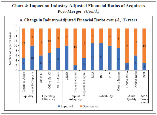
| Table 5: Acquirer’s Mean TE Pre- and Post-Merger | | Individual tests | Test groups | | Parametric Test | Non-Parametric Test | | t-test | Bootstrap t-test | Wilcoxon Signed-Rank Test | | Hypothesis | P(T ≤ t) | P(T ≤ t) | P(Z ≤ z) | | Test Statistics | Mean | t | Mean | t | Mean rank | z | | Short-term event window (-1,1) | | Pre-merger | 93.01 | -1.697 | 93.01 | -1.759 | 15.97 | -2.343** | | Post-merger | 94.55 | | 94.55 | | 19.03 | | | Short-term event window (-3,3) | | Pre-merger | 90.88 | -2.471** | 90.88 | -2.573** | 15.29 | -2.231** | | Post-merger | 93.80 | | 93.80 | | 19.71 | | | Medium-term event window (-3,5) | | Pre-merger | 90.88 | -3.172* | 90.88 | -3.266** | 14.68 | -2.397** | | Post-merger | 94.24 | | 94.24 | | 20.32 | | The results are statistically significant (Table 5). This improvement can be attributed to improvement in banks’ ability to curtail cost-inefficiency and better management practices. The results of the paper that mergers have, on an average, led to improvement in efficiency gains of acquirer banks are in contrast with the findings of Das and Kumbhakar (2022). This is partly due to methodological differences; while they used SFA, we used DEA. More importantly, however, their analysis focuses on the point that the acquired banks were more inefficient as compared with their acquirers. From this, they conclude that merger of inefficient banks with the more efficient banks may have pulled down the efficiency of the merged entity. While the present paper agrees with the findings of Das and Kumbhakar (2022) that typically the acquired entities were more inefficient than their acquirers, we show that this has not necessarily affected the efficiency of the merged entity. In section V.3, we show that, in fact geographical diversification and more focus on net interest income as earning source have improved the efficiency of the merged bank. Decomposing the post-merger TE scores into PTE and SE, the results indicate that the mean PTE of acquirers changed marginally from 98.85 in the pre-merger period to 98.82 three years post-merger and 98.85 five years post-merger. On the other hand, the mean SE of acquirers improved significantly from 92.11 in the pre-merger period to 95.15 three years post-merger and 95.37 five years post-merger (Chart 6 and Chart 7). These results, taken together indicate that relatively weak and inefficient acquiree banks were not a hindrance for efficiency of the merged entity and acquirers benefited from mergers primarily on account of increased scale of productive capacity.
The test results for PTE and SE scores also confirm the finding that there is no statistically significant difference in the pure technical efficiency of acquirer banks post-merger whereas the improvement in scale efficiency is statistically significant, both over the short-term and medium-term event window (Table 6 and Table 7). V.3: Does geographical diversification or focus on interest income explain efficiency gains? In order to investigate factors that may explain the efficiency improvement, a novel approach of panel-data Tobit regression was adopted with TE scores of acquirers as the dependant variable: where, GC is geographical concentration and NII/TI is the share of non-interest income to total income.13 Using state-wise branch spread of acquirers before and after merger, we constructed the Herfindahl-Hirschman index (HHI) of geographical concentration (GC). Thus, if the banks’ branches were concentrated in a few states, it gave a relatively higher HHI score as compared to a bank whose branches are spread widely across many states. An eyeball analysis suggests that the HHI of acquirer generally declined post-merger, implying that their geographical concentration reduced. Termed differently, merger resulted in geographical diversification for the acquirers. | Table 6: Acquirer’s Mean PTE Pre- and Post-Merger | | Individual tests | Test groups | | Parametric Test | Non-Parametric Test | | t-test | Bootstrap t-test | Wilcoxon Signed-Rank Test | | Hypothesis | P(T ≤ t) | P(T ≤ t) | P(Z ≤ z) | | Test Statistics | Mean | t | Mean | t | Mean rank | z | | Short-term event window (-1,1) | | Pre-merger | 98.75 | -0.200 | 98.75 | -0.205 | 17.76 | 0.267 | | Post-merger | 98.85 | | 98.85 | | 17.24 | | | Short-term event window (-3,3) | | Pre-merger | 98.85 | 0.088 | 98.85 | 0.090 | 18.21 | 0.351 | | Post-merger | 98.82 | | 98.82 | | 16.79 | | | Medium-term event window (-3,5) | | Pre-merger | 98.85 | -0.258 | 98.85 | -0.265 | 17.71 | 0.106 | | Post-merger | 98.95 | | 98.95 | | 17.29 | |
| Table 7: Acquirer’s Mean SE Pre- and Post-Merger | | Individual tests | Test groups | | Parametric Test | Non-Parametric Test | | t-test | Bootstrap t-test | Wilcoxon Signed-Rank Test | | Hypothesis | P(T ≤ t) | P(T ≤ t) | P(Z ≤ z) | | Test Statistics | Mean | t | Mean | t | Mean rank | z | | Short-term event window (-1,1) | | Pre-merger | 94.78 | -0.964 | 92.11 | -0.994 | 16.44 | -1.086 | | Post-merger | 95.73 | | 95.15 | | 18.56 | | | Short-term event window (-3,3) | | Pre-merger | 91.96 | -2.554** | 91.96 | -2.645** | 15.47 | -2.296** | | Post-merger | 94.95 | | 94.95 | | 19.53 | | | Medium-term event window (-3,5) | | Pre-merger | 91.96 | -2.647** | 92.11 | -2.747** | 15.29 | -2.462** | | Post-merger | 95.25 | | 95.37 | | 19.71 | | Elyasiani et al. (2012) used data on lending, securities and insurance activities of Bank Holding Companies (BHCs) to measure changes in production efficiency and found a negative association of TE with activity diversification. Data constraints however prevent us from using the same. Instead, we use the ratio of non-interest income to total income (NII/TI) as a proxy. The rationale behind this is that the primary business of banks is lending and any change in strategy that increases the share of interest income in total income may lead to increase in its efficiency. The expected sign of coefficient of this variable is negative. Apart from these factors, size of the bank (proxied by log of total assets) and a bank group dummy (0 for PSBs and 1 for PVBs) are used as control variables. | Table 8: Random Effects Tobit Regression for Acquirer’s TE over (-3,3) | | Dependent Variable: TE (-3,3) | | | (1) | (2) | (3) | (4) | | GC | -.303*** | -.344*** | | -.326*** | | | (.117) | (.117) | | (.12) | | Share of NII/TI | -.002 | | -.003** | -.002 | | | (.001) | | (.001) | (.001) | | Size | 0 | .002 | .01** | .001 | | | (.006) | (.006) | (.005) | (.006) | | Bank Group dummy | .053* | .044 | .044** | | | | (.028) | (.028) | (.022) | | | Constant | .991*** | .994*** | .844*** | 1.018*** | | | (.08) | (.082) | (.058) | (.083) | | Observations | 102 | 102 | 102 | 102 | | AIC | -314.06 | -313.70 | -307.94 | -312.71 | Note: 1. *** p<.01, ** p<.05, *p<.1
2. Figures in the parenthesis represent standard errors.
3. All the covariates are winsorised at the 95th percentile.
4. The TE scores were scaled down to lie between [0,1].
Source: Authors’ calculations. | The results indicate that post-merger geographical diversification and an increase in the share of interest income to total income led to improvement in efficiency. In particular, the negative coefficient of GC suggests that post-merger reduction in geographical concentration explains efficiency gains. Also given that the banking business is primarily focussed on lending activities, the diversification of banks away from non-interest income to interest income may have contributed to increased efficiencies (Table 8). The results are consistent across short-term as well as medium-term period (Table 9). In addition, the positive coefficient of asset size variable suggests that an increase in asset size post-merger helped in strengthening efficiencies. Gains in efficiencies were significantly higher for PVBs as compared with their PSB counterparts. V.4 How did the recent bank mergers perform? Since the recent spate of banking mergers (i.e., bank mergers during 2019-2020; refer to Annex II for details) attracted a lot of attention from analysts and researchers, we extended the analysis for these mergers as well, although longer time-series post-merger data as used in the earlier exercise is not yet available. Given that all the banks involved in the recent mergers were publicly listed, it is possible to evaluate the impact on shareholders’ wealth using the event study framework. An analysis of cumulative abnormal returns (CARs) one day prior and one day after the ‘news leak day’ suggested wealth gain for shareholders of the acquiree banks but losses for shareholders of the acquirer banks.14 This is not surprising in light of our earlier result that generally weak banks are acquired by stronger banks. Thus, the markets viewed the news of merger positively for the acquiree banks—in anticipation that their financials would strengthen after merger—but negatively for acquirer banks (Chart 8). | Table 9: Random Effects Tobit Regression for Acquirer’s TE over (-3,5) | | Dependent Variable: TE (-3,5) | | | (1) | (2) | (3) | (4) | | GC | -.164** | -.19** | | -.172** | | | (.078) | (.079) | | (.082) | | Share of NII/TI | -.003*** | | -.003*** | -.002** | | | (.001) | | (.001) | (.001) | | Size | .007 | .006 | .014*** | .007 | | | (.005) | (.005) | (.004) | (.005) | | Bank Group dummy | .048** | .034 | .044** | | | | (.022) | (.022) | (.02) | | | Constant | .9*** | .88*** | .804*** | .915*** | | | (.069) | (.07) | (.051) | (.072) | | Observations | 136 | 136 | 136 | 136 | | AIC | -439.34 | -434.61 | -436.67 | -434.45 | Note: 1. *** p<.01, ** p<.05, *p<.1
2. Figures in the parenthesis represent standard errors.
3. All the covariates are winsorised at the 95th percentile.
4. The TE scores were scaled down to lie between [0,1].
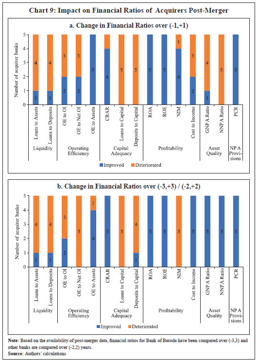
Source: Authors’ calculations. | Although longer time series data is not yet available for bank mergers between 2019-2020, the event study is complemented with financial ratio analysis and DEA using the data available so far. Financial ratio analysis suggests that CRAR, RoA, RoE, cost-to-income ratio, GNPA, NNPA and NPA provisions improved for the acquirers, post-merger (Chart 9). Moreover, the results are consistent across most of the metrics even after adjusting for industry-wide influences (Chart 10). Using limited data available so far, DEA analysis suggests that in four out of five cases under the study, acquirers were more efficient than the acquirees—in line with the historical trend presented earlier (Table 10). Test results of parametric and non-parametric tests also confirm that the differences in their efficiency are statistically significant (Table 11). | Table 10: Acquirer's vs Acquiree's Technical Efficiency Pre-Merger | | Merger | Pre-Merger | Acquirer's Pre-merger Average | Acquiree's Pre-merger Average | If Acquirer More Efficient than Acquiree Pre-Merger | | Acquirer | Acquiree | | 3 years | 2 years | 1 year | 3 years | 2 years | 1 year | | Merger 1 | 97.24 | 98.65 | 99.31 | 92.03 | 90.58 | 94.00 | 98.40 | 92.20 | Yes | | Merger 2 | 99.73 | 90.79 | 97.55 | 96.88 | 93.52 | 95.63 | 96.02 | 95.34 | Yes | | Merger 3 | 92.33 | 92.68 | 95.52 | 90.23 | 90.21 | 82.70 | 93.51 | 87.71 | Yes | | Merger 4 | 94.96 | 96.19 | 96.86 | 90.79 | 87.91 | 90.84 | 96.00 | 89.85 | Yes | | Merger 5 | 96.94 | 96.44 | 97.12 | 97.77 | 99.35 | 96.97 | 96.83 | 98.03 | No | | Note: In order to protect the financial interests of entities involved, mergers are neither arranged chronologically, nor alphabetically in this table, but randomly. |
 The DEA results also show that in most of the cases, the efficiency of acquirer has improved post-merger, and the difference is statistically significant (Tables 12 and 13). It may be noted that the results are based on limited data available so far and it is acknowledged that efficiency gains in some cases are yet to accrue and reflect in financial performance completely. Notwithstanding this disclaimer, it can be argued that recent mergers in the banking sector have contributed to efficiency gains.
| Table 11: Acquirer’s vs Acquiree’s Mean TE Pre-merger | | Individual tests | Test groups | | Parametric Test | Non-Parametric Test | | T-test | Bootstrap t-test | Mann- Whitney [Wilcoxon Rank-Sum] test | | Hypothesis | P(T ≤ t) | P(T ≤ t) | P(Z ≤ z) | | Test Statistics | Mean | t | Mean | t | Mean rank | z | | Pre-Merger (-3,0) | | | | | | | | Acquiree | 92.63 | -1.750* | 92.63 | -1.830* | 4 | -1.462* | | Acquirer | 96.15 | | 96.15 | | 7 | |
| Table 12: Acquirer TE Post-Merger | | | Pre-merger | Post-merger | Pre-merger Average | Post-merger Average | Change in Efficiency | | 3 years | 2 years | 1 year | 1 year | 2 years | 3 years | | Merger 1 | 94.96 | 96.19 | 96.86 | 92.28 | 93.06 | 88.13 | 96.00 | 91.16 | Decreased | | Merger 2 | | 90.79 | 97.55 | 96.54 | 98.46 | | 94.17 | 97.50 | Increased | | Merger 3 | | 92.68 | 95.52 | 93.55 | 98.13 | | 94.10 | 95.84 | Increased | | Merger 4 | | 96.44 | 97.12 | 96.57 | 98.12 | | 96.78 | 97.34 | Increased | | Merger 5 | | 98.65 | 99.31 | 96.25 | 96.52 | | 98.98 | 96.39 | Decreased | Note: 1. In order to protect the financial interests of entities involved, mergers are neither arranged chronologically nor alphabetically in this table, but randomly.
2. Based on the availability of post-merger data, financial ratios for Bank of Baroda have been compared over (-3,3) and other banks are compared over (-2,2) years.
Source: Authors’ calculations. |
| Table 13: Acquirer’s Mean TE Pre- and Post-Merger | | Individual tests | Test groups | | Parametric Test | Non-Parametric Test | | t-test | Bootstrap t-test | Wilcoxon Signed-Rank Test | | Hypothesis | P(T ≤ t) | P(T ≤ t) | P(Z ≤ z) | | Test Statistics | Mean | t | Mean | t | Mean rank | z | | Pre-merger | 96.01 | 0.243 | 96.01 | 0.272 | 5.4 | -0.135 | | Post-merger | 95.65 | | 95.65 | | 5.6 | | Section VI
Conclusions Compiling data on bank mergers during 1997-2020, comprising both public and private sector banks, the current study employs DEA, financial ratio technique and event study analysis to investigate the impact of bank mergers in the Indian context. The study also uses a novel technique of panel Tobit regression to assess the factors that may have contributed to efficiency gains in the post-merger period. In particular, the paper seeks to answer four questions: a) What were the efficiency characteristics of acquirer and acquiree banks pre-merger? In particular, whether the mergers were amongst equals or between a strong and a weak bank?; b) Whether the financial performance and efficiency of acquirers improved or deteriorated post-merger and what contributed to these efficiency gains – improvement in managerial prowess or scale efficiencies?; c) Did geographical diversification and/or greater focus on interest earnings post-merger contribute to efficiency improvement?; and d) How successful were the recent mergers? The findings of the paper confirm that banking mergers in India have been, on an average, beneficial to the banking sector as the financial performance and efficiency of acquirers improved post-merger. These findings also hold true for the recent bank mergers during 2019-2020, for which limited data is available so far. Our findings suggest that the mean technical efficiency of acquirers increased from 90.88 in the pre-merger period to 93.80 three years post-merger, and 94.24 five years post-merger. Relatively lower managerial and organisational competencies in acquired banks were not a hindrance for preserving efficiency of the merged entity and the benefits to acquirers from mergers on account of increased scale of productive capacity were statistically significant. A deep dive into factors that may have led to efficiency gains identifies post-merger geographical diversification and improvement in the share of interest income as the significant factors. An analysis of cumulative abnormal returns one day prior and one day after the ‘news leak day’ in the event study framework for banks that merged during 2019-2020 suggested wealth gains for the shareholders of the acquiree banks. This is not surprising in light of our earlier results that generally weak banks were acquired by stronger banks. Thus, the markets viewed the news of merger positively for the acquiree banks, in anticipation that their financials would strengthen after merger. The evidence so far, thus, suggests that mergers have been an effective tool of efficiency improvement in the Indian banking sector. Mergers have provided avenues for increasing the scale of operations, geographical diversification, and adoption of more efficient business strategies.
References Akhavein, J., Berger, A., & Humphrey, D. (1997). The effects of megamergers on efficiency and prices: evidence from a bank profit function. 12(1), 95–139. Alexander, W. R. J., & Joforullah, M. (2005). Scale and pure efficiencies of New Zealand secondary schools. (Discussion Paper No. 0501). University of Otago. Al-Sharkas, A., & Hassan, M. (2010). New evidence on shareholder wealth effects in bank mergers during 1980–2000. 34(3), 326-348. Al-Sharkas, A., Hassan, M., & Lawrence, S. (2008). The impact of mergers and acquisition on the efficiency of the US banking industry: further evidence. 35(1/2), 50-70. Amihud, Y., DeLong, G., & Saunders, A. (2002). The effects of cross-border bank mergers on bank risk and value. J Int Money Financ, 21(6), 857-877. Antil, S., Kumar, M. & Swain, N. (2020) Evaluating the efficiency of regional rural banks across the Indian states during different phases of structural development, Applied Economics, 52:41, 4457-4473. Avkiran, N. (1999). The evidence on efficiency gains: the role of mergers and the benefits to the public. Journal of Banking and Finance, 23, 991-1013.. Avkiran, N.K. (2006). Productivity analysis in the service sector with Data Envelopment Analysis. Available at SSRN: https://ssrn.com/abstract=2627576 Azofra, S., Olalla, M., & Olmo, B. (2008). Size, Target Performance and European Bank Mergers and Acquisitions. American Journal of Business, 53-63. Bauer, P. W., Berger, A. N., Hamphrey, D.B., & Ferrier, G.D. (1998). Consistency conditions for regulatory analysis of financial institutions. Journal of Economics and Business, 50, 85-114. Benston, G. J. (1965). Branch Banking and Economies of Scale. The Journal of Finance 20 (2): 312–331. Berger, A. N., Saunders, A., Scalise, J. M., & Udell, G. F. (1998). The effects of bank mergers and acquisitions on small business lending. Journal of Financial Economics, 187-229. Bhattacharyya, A., Lovell, C., & Sahay, P. (1997). The impact of liberalization on the productive efficiency of Indian commercial banks. European Journal of Operational Research, Elsevier, vol. 98(2), pages 332-345, April. Bishnoi, R. T., & Devi, S. (2015). Mergers and Acquisitions of Banks in Post-Reform India. Economic and Political Weekly, 50-58. Boyd, J., H., Graham, S., L. (1988) The profitability and risk effects of allowing bank holding companies to merge with other financial firms: a simulation study. Fed Reserve Bank Minneap Q Rev 12(2):3–20. Campa J., M., Hernando, I. (2006) M&As performance in the European financial industry. J Bank Financ 30(12):3367–3392. Chen, Y. & Ali, I., A. (2002). Output-input ratio analysis and DEA frontier. European Journal of Operational Research, Elsevier, vol. 142(3), pages 476-479, November. Cornett, M., & Tehranian, H. (1992). Changes in corporate performance associated with bank acquisitions. J Financ Econ, 31(2), 211–234. Cornett, M. M., McNutt, J. J., & Tehranian, H. (2006). Performance Changes around Bank Mergers: Revenue Enhancements versus Cost Reductions. Journal of Money, Credit and Banking, 38(4), 1013–1050. Das, A., Kumbhakar, S., C. (2022). Bank Merger, Credit Growth, and the Great Slowdown in India. Economic and Political Weekly, Volume 57, Year 2022, Pages 58-67. DeLong, G. (2003a). The announcement effects of US versus non-US bank mergers: do they differ? J Financ Re, 26(4), 487–500. DeLong. (2003b). Does long-term performance of mergers match market expectations? Evidence from the U.S. banking industry. Financial Management 32, 5–25., 32, 5-25. DeYoung, R. (1997) Bank mergers, x-efficiency, and the market for corporate control. Manag Financ 23(1):32–47. DeYoung, R., Evanoff, D., D. & Molyneux, P. (2009). Mergers and Acquisitions of Financial Institutions: A Review of the Post-2000 Literature. J Financ Serv Res 36, 87–110. Elyasiani, E., & Wang, Y. (2012). Bank holding company diversification and production efficiency. Applied Financial Economics, 22:17, 1409-1428. Reserve Bank of India, (2008). Report on Currency and Finance.. Fixler, D., & Zieschang, K. (1993). An index number approach to measuring bank efficiency: an application to mergers. J Bank Financ, 23(4), 367–386. Fried, H., Lovell, C., & Yaisawarng, S. (1999). The impact of mergers on credit union service provision. J Bank Financ, 23(4), 367–386. Goddard, J., Molyneux, P., & Zhou, T. (2012). Bank mergers and acquisitions in emerging markets: evidence from Asia and Latin America. Eur J Financ, 18(5), 419–438. Gurkaynak, R., & Wright, J. (2013). Identification and inference using event studies. 81, 48–65. Hannan, T., & Wolken, J. (1989). Returns to bidders and targets in the acquisition process: evidence from the banking industry. J Financ Serv Res, 3(1), 5–16. Haynes, M., & Thompson, S. (1999). The productivity effect of bank mergers: evidence from the UK building societies. J Bank Financ, 23(5), 825–846. Houston, J., & Ryngaert, M. (1994). The overall gains from large bank mergers. J Bank Financ, 18(6), 1155–1176. Houston, J., & Ryngaert, M. (1997). Equity issuance and adverse selection: a direct test using conditional stock offers. J Financ, 52(1), 197–219. Houston, J., James, C., & Ryngaert, M. (2001). Where do merger gains come from? Bank mergers from the perspective of insiders and outsiders. J Financ Econ, 60(2/3), 285–331. Isik, I., & Hassan, M. (2002). Technical, scale and allocative efficiencies of Turkish banking industry. Journal of Banking and Finance, 26, 719–66. Ismail, A., & Davidson, I. (2005). Further analysis of mergers and shareholder wealth effects in European banking. Appl Financ Econ, 15(1), 13–30. Ismail, A., & Davidson, I. (2007). The determinants of target returns in European bank mergers. Serv Ind J, 27(5), 617–634. Jayaraman, A., & Srinivasan, M. R. (2014). Impact of merger and acquisition on the efficiency of Indian bank: a pre -post analysis using data envelopment analysis. Int. J. Financial Services Management, 7 (1). Joshua, O. (2011). Comparative Analysis of the Impact of Mergers and Acquisitions on Financial Efficiency of Banks in Nigeria. Journal of Accounting and Taxation, 3, 1-7. Kao, C., & Liu, S. (2004). Predicting Bank Performance with Financial Forecasts: A Case of Taiwan Commercial Banks. Journal of Banking & Finance, 28 (10), 2353–2368. Kashyap, N. & Mahapatro, S. & Tantri, P. (2022). How Does The Rescue of Weak Banks Through Mergers Impact Loan Performance? Evidence From India *. Kiymaz, H. (2004). Cross-border acquisitions of US financial institutions: impact of macroeconomic factors. J Bank Financ, 28(6), 1413–1439. Kiymaz, H. (2013). Cross-border mergers and acquisition and country risk ratings: evidence from US financials. Int J Bus Financ Res, 7(1), 17–29. Knapp, M., Gart, A. & Becher, D. (2005). Post-Merger Performance of Bank Holding Companies, 1987-1998. The Financial Review, Eastern Finance Association, vol. 40(4), pages 549-574, November. Kolaric, S. & Schiereck, D. (2013). Shareholder wealth effects of bank mergers and acquisitions in Latin America. Management Research: The Journal of the Iberoamerican Academy of Management, 11(2), 157-177. Kolaric, S. & Schiereck, D. (2014). Performance of bank mergers and acquisitions: a review of the recent empirical evidence. Manag Rev Q, 39-71. Kondova, G., G. & Burghof, H., P. (2007) The impact of bank mergers on efficiency: empircial evidence from the German banking industry. In: Conference paper presented at the EFMA annual meeting 2007, Vienna Kumar, M., Kumar, S. & Deisting, F. (2013). Wealth effects of bank mergers in India: A study of impact on share prices, volatility and liquidity. Banks and Bank Systems, 8(1), 127–133. Kwan, S., & Wilcox, J. (1999). Hidden cost reductions in bank mergers: accounting for more productive banks. Working Papers in Applied Economic Theory 99-10, Federal Reserve Bank of San Francisco. Lancaster, T. (2000). The incidental parameter problem since 1948. Journal of Econometrics, 95, 391–413. Leeladhar, V. (2008). Consolidation in the Indian Financial Sector. Adress at the International Banking & Finance Conference. Indian Merchants’ Chamber, Mumbai. Lee, T., H., Liang, L., W. & Huang, B., Y. (2013). Do mergers improve the efficiency of banks in Taiwan? Evidence from stochastic frontier approach. The Journal of Developing Areas, 47(1), 395–416. Linder, J. & Crane, D. (1993). Bank mergers: integration and profitability. J Financ Serv Res, 7(1), 35–55. Liu, B. & Tripe, D. (2003). New Zealand Bank Mergers and Efficiency Gains. Journal of Asia-Pacific Business, 37-41. MacKinlay, A. (1997). Event Studies in Economics and Finance. Journal of Economic Literature, 35(1), 13–39. Mathur, A., Sengupta, R. & Pratap, B. (2021). Saved by the bell? Equity market responses to surprise Covid-19 lockdowns and central bank interventions. . Mester, L. (1987). Efficient production of financial services: scale and scope economies. Federal Reserve Bank of Philadelphia Business Review, 15-25. Nataraja, N., R., & Johnson, A., L. (2011). Guidelines for Using Variable Selection Techniques in Data Envelopment Analysis. European Journal of Operational Research, 215 (3), 662–669. Neyman, J., & Scott, E. (1948). Consistent Estimates Based on Partially Consistent Observations. Econometrica, 16, 1-32. Nishat, Shabnam, The Impact of Mega Mergers on the Efficiency of Indian PSU Banks (March 22, 2020). IUP Journal of Business Strategy. Jun2020, Vol. 17 Issue 2, p21-33. 13p Peristiani, S. (1997). Do mergers improve the x-efficiency and scale efficiency of US banks? Evidence from the 1980s. J Money Credit Bank, 29(3), 326–337. Reda, M. (2013). The effect of mergers and acquisitions on bank efficiency: evidence from bank consolidation in egypt. The Economic Research Forum (ERF), 1-24. Rhoades, S. (1998). The efficiency effects of bank mergers: An overview of case studies of nine mergers. Journal of Banking and Finance, 22, 273–291. Sameer Mohammed Sindi & A.N. Bany-Ariffin & Nazrul Hisyam Ab Razak & Fakarudin Kamarudin. (2021). Bank mergers and acquisitions in emerging markets: evidence from the Middle East and the North Africa region, International Journal of Business and Globalisation, vol. 28(1/2), pages 97-116. Sathye, M. (2001). X-efficiency in Australian banking: An empirical investigation. Journal of Banking and Finance. Journal of Banking and Finance, 25, 613–630. Sathye, M. (2003). Efficiency of Banks in a Developing Economy: The Case of India. European Journal of Operational Research, 148 (3), 662–671. Schiereck, S. K. (2014, January). Performance of bank mergers and acquisitions: a review of the recent emprical evidence. 39-71. doi:10.1007/s11301-014-0099-3 Seadly, C., & Lindley, J. (1977). Inputs, outputs and a theory of production and cost at depository financial institutions. Journal of Finance, 32, 1251±1266. Singh, P. (2009). Mergers in Indian Banking: Impact Study using DEA Analysis. South Asian journal of management. Vol. 16.2009, 2, p. 7-27. Sonia Antil, Mukesh Kumar & Niranjan Swain. (2020). Evaluating the efficiency of regional rural banks across the Indian states during different phases of structural development, Applied Economics, 52:41, 4457-4473, Sufian, F., & Habibullah, M. (2009). Asian financial crisis and the evolution of Korean banks efficiency: A DEA approach. Global Economic Review, Taylor and Francis Journals, 38 (4), 335-69. Sufian, F. (2007). Mergers and acquisitions in the Malaysian banking industry: technical and scale efficiency effects. International Journal of Financial Services Management, 304-326. Thanassoulis, E., Boussofiane, A., & Dyson, R. (1996, June). A comparison of data envelopment analysis and ratio analysis as tools for performance assessment. Omega, Elsevier, 24 (3), 229-244. Wanke, M. G. (2017). Merger and acquisitions in South African banking: A network DEA model. Research in International Business and Finance, 362-376.
Annexure | Annex I: List of M&As during 1997-2017 | | Sr. No. | Name of Transferor Bank/ Institution | Name of Transferee Bank/ Institution | Date of Amalgamation | Merger Type | | 1 | Punjab Co-operative Bank Ltd. | Oriental Bank of Commerce | April 8, 1997 | PVB to PSB | | 2 | Bareilly Corporation Bank Ltd. | Bank of Baroda | June 3, 1999 | PVB to PVB | | 3 | Times Bank Ltd. | HDFC Bank Ltd. | February 26, 2000 | PVB to PVB | | 4 | Bank of Madura Ltd. | ICICI Bank Ltd. | March 10, 2001 | PVB to PVB | | 5 | Benares State Bank Ltd. | Bank of Baroda | June 20, 2002 | PVB to PSB | | 6 | Nedungadi Bank Ltd. | Punjab National Bank | February 1, 2003 | PVB to PSB | | 7 | Global Trust Bank Ltd. | Oriental Bank of Commerce | August 14, 2004 | PVB to PSB | | 8 | Ganesh Bank of Kurundwad Ltd. | Federal Bank Ltd. | September 2, 2006 | PVB to PVB | | 9 | United Western Bank Ltd. | IDBI Ltd. | October 3, 2006 | PVB to PSB | | 10 | Bharat Overseas Bank Ltd. | Indian Overseas Bank | March 31, 2007 | PVB to PVB | | 11 | Sangli Bank Ltd. | ICICI Bank Ltd. | April 19, 2007 | PVB to PVB | | 12 | Centurion Bank of Punjab Ltd. | HDFC Bank Ltd. | May 23, 2008 | PVB to PVB | | 13 | State Bank of Saurashtra | State Bank of India | August 13, 2008 | PSB to PSB | | 14 | Bank of Rajasthan | ICICI Bank | August 12, 2010 | PVB to PVB | | 15 | State Bank of Indore | State Bank of India | August 26, 2010 | PSB to PSB | | 16 | ING Vysya Bank | Kotak Mahindra Bank | April 01, 2015 | PVB to PVB | | 17 | State Bank of Bikaner and Jaipur
State Bank of Hyderabad
State Bank of Mysore
State Bank of Patiala
State Bank of Travancore
Bhartiya Mahila Bank | State Bank of India | April 01, 2017 | PSB to PSB | Note: PSB: Public Sector Bank, PVB: Private Sector Bank
Source: STRBI, Various Issues. |
| Annex II: List of Bank M&As during 2019-2020 | | Sr. No. | Name of Transferor Bank/ Institution | Name of Transferee Bank/Institution | Official Announcement Date | Date of Amalgamation | Merger Type | | 1 | Vijaya Bank
Dena Bank | Bank of Baroda | January 02, 2019 | April 01, 2019 | PSB to PSB | | 2 | Oriental Bank of Commerce
United Bank of India | Punjab National Bank | August 30, 2019 | April 01, 2020 | PSB to PSB | | 3 | Syndicate Bank | Canara Bank | August 30, 2019 | April 01, 2020 | PSB to PSB | | 4 | Andhra Bank
Corporation Bank | Union Bank of India | August 30, 2019 | April 01, 2020 | PSB to PSB | | 5 | Allahabad Bank | Indian Bank | August 30, 2019 | April 01, 2020 | PSB to PSB | Note: The merger between Lakshmi Vilas Bank and DBS India Pvt. Ltd., being a M&A transaction between PVB to FB, was not considered for the study.
Source: STRBI, Various Issues. | Annex III: Definitions of Financial Ratios a) Liquidity Ratios: Measures changes in banks’ cash position i) Loans to Assets = Net Loans and Advances/Total Assets ii) Loans to Deposits = Net Loans and Advances/Total Deposits b) Profitability Ratios15: Measures the overall performance of the bank i) Return on Assets (ROA) = Net Profit after tax / Total Assets ii) Return on Equity (ROE) = Net Profit after tax / Total Capital + Reserves and Surplus iii) Net Interest Margin (NIM) = (Interest Earned – Interest Expended) 100*/Total Assets iv) Cost to Income = Non-Interest Expense* 100 /Net Operating Income c) Operating Efficiency Ratios: Measures the ability of bank managers to reduce costs and thus approximates employee productivity. i) Operating Expense to Operating Income = Non-Interest Expense/Non-Interest Income ii) Operating Expense to Net Operating Income = Non-Interest Expense/Net Operating Income iii) Operating Expense to Total Assets = Non-Interest Expense/Total Assets d) Capital Adequacy: Measures the ability of banks to absorb potential losses while remaining solvent and meet regulatory standards i) Capital to Assets = Total Capital/ Total Assets ii) Loans to Capital = Net Loans and Advances/Total Capital iii) Deposits to Capital = Total Deposits/ Total Capital e) Asset Quality: Measures changes in a bank’s loan quality and credit risk associated with the lending business i) GNPA ratio = Gross Non-performing Assets (NPAs)/ Gross Loans & Advances ii) NNPA ratio = Net NPAs16/ Net Loans & Advances f) NPA Provisions: Measures the ability of banks to provision against loss-making assets and also to meet regulatory standards. i) Provision Coverage Ratio (PCR) = Total NPA provisions/Gross NPAs Annex IV: DEA Methodology
|