Press Release

RBI Working Paper Series No. 01

Measuring Contagion Effects of Crude Oil Prices on Sectoral Stock Price Indices in India

Madhuchhanda Sahoo, Arvind Kumar Shrivastava, Jessica Maria Anthony and Thangzason Sonna^@

Abstract

¹This paper explores the contagion effects of extreme changes in global crude oil prices on sectoral stock price indices in India. Using generalised Pareto distribution (GPD) for estimating excess returns or exceedances i.e., deviations from thresholds, and multinomial logit model (MNL) for assessing the probability of contemporaneous excess returns or co-exceedances, the paper finds a significant likelihood of co-exceedances among 10 sectoral stock price indices when faced with extreme changes in global crude oil prices. This points to the existence of a contagion effect. The evidence of positive co-exceedances is stronger, and the results are found more robust when relevant control variables are introduced – exchange rate returns (INR-USD), 10-year G-sec yield, and differential stock returns, (i.e., small firms minus big firms (SMB)). The contagion effect on all sectoral indices, irrespective of their direct and indirect exposure to oil price dynamics, highlights the need for hedging by investors as mere diversification of portfolios may not be sufficient to protect their assets from an adverse oil price shock.

JEL classification: C32, G12, G15

Introduction

The studies on contagion effects of extreme changes in global prices of crude oil on sectoral stock indices done in the Indian context are rare. There are not many studies on this subject even at the international level. The increasing cross-border financial integration warrants that the contagion effects of global prices of crude oil – one of the most actively traded commodities worldwide - on stock prices is understood better. For an oil-dependent economy like India, importing around 80 per cent of its consumption requirements, the need for a deeper understanding of the contagion effects of global crude oil prices is all the more pressing.

Oil has both commodity and financial attributes. As a commodity, while rising oil price increases the operating costs of firms leading to depressed stock prices, as a financial asset, when higher oil price is driven by higher demand expansion, it positively affects stock returns. Studies have observed that crude oil shocks can influence expected earnings in the equity markets, both within and across borders, while the macroeconomic impact of oil price shocks can also have ramifications for overall liquidity in the financial market.

Commensurate with being the second-largest country in the world in terms of population, the fifth-largest economy in the world, and third in Asia, India holds the distinction of being the third-largest consumer of oil, next only to China and the US. Likewise, India is the third-largest importer of crude oil after the US and China. Domestically, oil is the largest source of the country’s total energy supply next only to coal and also is the largest in terms of total final consumption. The demand for oil is increasing rapidly. Yet, owing to low natural endowment and stagnant domestic production, India’s reliance on imports for meeting the demand-supply gap is high. Also, the oil and gas sector is one of the six core industries in India and is among the most traded commodities. It is, therefore, natural that the implications of extreme changes in global prices of crude oil on the Indian macro economy would be profound. In the same vein, it may not be farfetched to expect movements in global prices of crude oil to impact Indian stock indices. More so because the Indian stock market has grown larger, and the Indian financial system is substantially integrated with the global financial system over the years.

In this backdrop, with the motivation to empirically examine the existence of contagion effect of extreme changes in global crude oil returns on 10 composite sectoral indices of Indian stock markets, the paper employs the multinomial logit model (MNL), as in Sheng Fang and Paul Egan (2018) for China. The threshold returns for global crude oil price and sectoral stock indices – both for the top and bottom tails, are established using a generalised Pareto distribution (GPD) function. Having established the thresholds, the MNL model is used to examine the probability of extreme returns or exceedances, defined as deviation from thresholds, contemporaneously occurring among the stock sectors due to exceedances in oil price returns, which the literature has defined as contagion effects.

The study has been organised into five sections. Section II presents the review of the literature and the stylised facts. Section III provides a detailed explanation of methodology, data, and preliminary analysis. Section IV reports and analyses the empirical results and Section V concludes the paper.

II. Review of Literature and Stylised Facts

II.1 Review of Literature

Hamilton (1983) discovered that crude oil price changes played a key role during every post-World War-II US recession. After his pioneer work, exploring the linkages between crude oil price and the real sectors of the economy has been a major area of theoretical and empirical research. Successive researchers investigated the association between oil price shocks and macroeconomic variables - economic growth, aggregate demand, inflation, and employment in various countries. The subsequent studies that followed, established without ambiguity that oil price shock has the potential to trigger cost-push inflation, adversely affecting profitability and causing generalised inflation. And if unchecked, it can engulf the whole economy, leading to higher unemployment, compressed demand, and consumption, discouraging investment, and a sustained growth slowdown.

Indeed, the crude oil price surge due to the Arab oil embargo was at the core of the global slowdown during 1974-75. The global Gross Domestic Product (GDP) grew by 6.9 per cent in 1973, fell to 2.1 per cent in 1974, and to 1.4 per cent in 1975. It was only by 1976 after the oil embargo that the world economy returned to its normal rate of growth. The US GDP contracted for three consecutive years during 1973-75 and unemployment and inflation rates more than doubled. So pervasive was the impact that it led to an aspersion on the foundation of Classical Economics, according to which inflation is always and everywhere a monetary phenomenon, and its off-shoot – the Philips Curve – which assumed a steady, permanent, and direct relationship between employment and inflation.

The studies on the relationship between volatility in crude oil price movements and stock indices have been relatively of a new vintage as compared to studies on the relationship between crude oil price movements and macroeconomic variables. The premise that the rise in performance of the stock market is a good indicator of economic activity, has existed all along as a perceived notion. In fact, this notion led to another perceived notion of the existence of a causal relationship between crude oil price and the stock market. Studies like Nasseh and Strauss (2000); Pethe and Karnik (2000); Singh (2010); Dhiman and Sahu (2010) have attempted to empirically examine the relationship between crude oil price and macroeconomic variables in different countries including India. Most studies observed a strong relationship between crude oil price movements and macroeconomic variables.

As regards crude oil price movements and stock markets, the empirical literature has been vast, and the findings thereof point mostly to an inverse relationship. There have, however, been a few studies that have found the relationship to be non-existent as well. Commonly, the relationship between the two markets has been analysed using (a) extreme returns on crude oil price, frequent fluctuations in crude oil prices, the net external trading position of the country in the global crude oil market (exporter or importer), and origin of crude oil price shocks (demand or supply-driven) on the one hand, and (b) overall returns or volatility of stock markets on the other, with relevant control variables like foreign currency exchange rate and interest rate.

A study on stock markets of the Gulf Cooperation Council (GCC) pointed out that negative oil price change had a larger negative impact on the stock markets of Kuwait, Oman, and Qatar which being oil exporting countries are relatively more responsive to the considerable oil price change (IMF WP, 2018). The stock markets of Latin American countries have been found to respond positively to increases in oil prices during 2000-2015 (Salgado et al., 2017). According to the authors, their finding can be explained based on regional closeness, shared institutional, historical and cultural features, and the way country-funds and regional-funds managers and other institutional investors who hold Latin American stocks react to oil price shocks.

Examining the differential impacts of fluctuations in crude oil prices on oil-importing and exporting countries, Asteriou, Dimitras, and Lendewig (2013) observed that the impact was higher for countries importing crude oil than countries exporting it and that the relationship between oil price and stock markets was more robust than between various interest rates – both in the short and long-runs. Imarhiabel (2010) also examined the effect of crude oil prices on the prices of stocks of select major oil-producing and consuming countries such as Mexico, Russia, Saudi Arabia, India, China, and the United States, and detected that stock prices were affected by both oil prices and currency exchange rates. Further, a time-series study of almost three decades by Thorbecke (2019) highlighted that the US stock markets got negatively affected by shocks in oil price during 1990-2007, but after that, they were positively affected during 2010 to 2018 indicating a change in nature of the relation. This finding, according to the author was explained by the rise of shale oil production and the changed structure of US economy - stocks in many sectors that were harmed by oil price increases before the Shale revolution benefited in the latter period.

Even for India, the relationship between the two markets has been negative according to most studies. A study by Rai and Bairagi (2014) showed a significant correlation between a crude oil price change and Bombay Stock Exchange (BSE) Sensex for the period 2003 to 2012. Another study by Sathyanarayana et al. (2018) spoke of a positive, significant, and direct relationship between crude oil and BSE Sensex, with an increase in oil price leading to an increase in share market price. Fluctuations in crude oil price return exerted a significant impact on the volatility of stock market returns in India and such volatility spillovers were stronger following the global financial crisis (Anand et al., 2014).

But there have been exceptions. According to Chittendi (2012), volatile stock prices did not necessarily have a significant impact on oil price volatility and there was no long-run equilibrium relationship between international crude oil price and the Indian stock market during 2003 to 2011, although such a relation was observed during 2008-2011 (Ghosh and Kanjilal, 2016). Surprisingly, oil demand shocks, but not supply shocks, affected stock returns in India and its volatility, despite the fact that policy uncertainty could lead to negative returns and increased volatility (Anand et al., 2021).

Despite being a vastly studied topic, the precise relationship between crude oil price volatility and stock prices and the contagion effect thereof has not been stated with certainty. This has prompted a new approach to study the two markets i.e., to take into consideration industry-specific stock prices. The widely held view is that the sectoral segregation of stock market indices is necessary to gain a deeper knowledge of the impact of crude oil price fluctuations.

However, even in this regard, there have been not many studies in the Indian context. Studies exist for other countries, such as the US, Europe, and China. A study by Degiannakis et al. (2013) highlights the importance of the sectoral division of the stock market with regard to various industries as an important determinant in determining the nature of the association between prices of international crude oil and the stock market. They examine equity returns of 10 European industrial sectoral indices and their linkages with oil price changes via the Diag-VECH GARCH model and conclude that relationships are industry-specific. Another study on the relationship of European sectoral stocks with crude oil prices is found to be asymmetric (Arouri, 2011) and strongly varying across sectors. While Automobiles and parts, Financials, Food and Beverages, and Health care show a negative relationship, Oil and Gas show a positive relationship.

In another study by Thorbecke (2019), a positive relationship between crude oil price volatility and stock prices were seen for industries that acted as an input to the energy sector, such as industrial machinery and marine transport and industries in the oil supply chain (petrochemicals). Kang et al. (2017) concluded that the index for the oil and gas industry responded negatively to negative supply-side shocks and positively to positive aggregate demand shocks for the US.

It was also found that stock prices of manufacturing, chemical, medical, food, transportation, computer, real estate, and general services responded negatively to a rise in oil prices, whereas the results were indeterminate for stock prices of engineering, electricity, and financial sectors by using 56 firm-level stocks of the US (Narayan and Sharma, 2011). In one interesting time-series study by Singhal and Ghosh (2016), the relation of seven industry-specific sectoral stock prices of BSE with crude oil prices was examined and significant empirical evidence was obtained.

Yet in another study, Rajan and Lourthuraj (2020) have tried to understand the impact of crude oil price on the automotive sector and companies’ performances. Jambotkar and Anjana (2018) also through an empirical analysis studied the combined effects of macro-economic variables, including crude oil prices on selected National Stock Exchange (NSE) sectoral indices and found significant results. A recent paper by Fang and Egan (2018) investigated the contagion effects using extreme positive and negative returns and the multinomial logit model (MNL) for 10 Chinese stock sectoral indices. The theory of extreme value has been used the least to understand the oil price spill over on sectoral stock prices in the case of Indian stock markets. It was used only in a few other countries and other fields like Horvath et al. (2018) and Chan-Lau et al. (2012). In addition to this, the literature shows that very few studies exist on the impact of crude oil prices on cross-market linkage i.e., inter-sectoral linkage for extreme returns in crude oil prices for India’s stock markets.

Hence, a study of sectoral stock price indices and an attempt to measure inter-sectoral linkages are key to understanding the nature of the relationship between oil prices and industry-specific sectoral stock markets. This paper is a step in that direction.

II.2 Stylised Facts

The Indian stock market has grown significantly in the last two decades. The number of listed companies in the NSE is more than 1900 while its benchmark index, Nifty comprises 50 companies. The NSE also has many sectoral and thematic indices. Similarly, BSE’s Sensex is a weighted stock market index of 30 well-established listed companies. The BSE is among the world's 10 largest exchanges in terms of the cumulative market capitalisation of all companies listed on its platform, as per the latest data available from the World Federation of Exchanges. The NSE has maintained the position of the largest derivatives exchange during 2019 and 2020 in terms of the number of contracts traded.

The BSE has the largest number of listed companies in the world (in the case of equities and debt). BSE is also the fastest exchange in the world with a median response time to trade of 6 microseconds. The NSE was by far the largest exchange in terms of stock index options trading, with over 1.85 billion contracts traded in H1 2019.

The average daily turnover in NSE was ₹57,677 crore and market capitalisation was ₹2,55,68,863 crore as on end-May 2022 and for BSE, the average daily turnover was ₹4,192.1 crore and the market capitalisation was at ₹2,57,78,368 crore in the same period. The stock market capitalisation to GDP ratio for BSE has improved significantly from 24 per cent in 1992-93 to 104.9 per cent in 2020-21.

Apart from these milestones, the co-movement of Indian stock indices with global crude oil price (Brent) and these indices getting affected by major global events make it even more necessary to study the relationship between these indices and global crude oil price (Chart 1).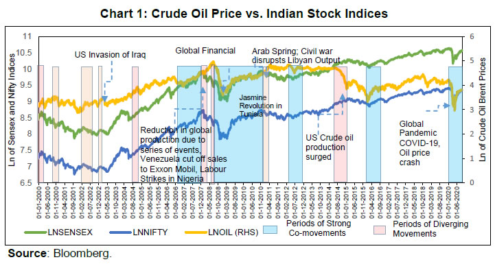

The contagion impact of global crude oil price on stock indices at the sectoral level is also backed by theory. There are two prominent theories supporting the linkage of international crude oil price movements and sectoral/industry-specific trends in stock indices. The first one, the channel of Expected Cash Flows states that the rise in oil prices leads to a rise in the cost of production, which in turn can reduce profit margins and hence cash flows (Dadashi et al., 2015). Theoretically, oil marketing, paints, synthetic rubber (tires), and the aviation industry’s input costs might rise due to a surge in crude oil price and their stock prices fall with rise in global crude oil price. Similarly, oil production and exploration companies may profit from a rise in crude oil prices and their stock prices may rise. The second theory of Discounted Future Cash Flows says that high oil prices can lead to inflationary expectations and hence rise in the interest rate, ultimately leading to higher borrowing costs.

The ultimate response of stock prices to crude oil price shocks, however, would depend upon whether the company is oil-producing or consuming. More importantly, the input-output coefficient of that sector would determine the responsiveness of its stock to oil price shocks. The volatility in oil prices can affect the operating costs of firms – both oil-producing and consuming and hit their earnings. Similarly, the profit and dividends of firms that use oil as inputs – direct or indirect, are bound to be impacted by volatility in oil prices. Likewise, the volatility in oil prices for an oil-importing or exporting market will differ widely. An upward movement in oil prices, while increasing risk and uncertainty in oil-importing markets, will increase market returns for an oil-exporting market. With a view to exploring these aspects of the behaviour of oil price movements on sectoral stock indices, 10 sectoral stock indices from BSE/NSE have been mapped against the input-output coefficient of India (MOSPI, 2012) taking petroleum products as the input. The input-output coefficients² across eight sectors were estimated (Chart 2).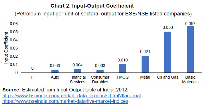

The higher input-output coefficients for Oil and Gas, and Basic Materials are on expected lines since the input intensity of petroleum products in these sectors is higher than in other sectors, such as IT and Financial Services. However, a broadly similar returns pattern can be observed across all stock sectors as well as Brent crude returns despite higher volatility in crude returns. All the 10 stock sector returns shared a statistically significant and positive correlation with Brent crude returns ranging between 0.11 to 0.20, indicative of the presence of contagion effect from extreme changes in global crude oil prices (Chart 3). Excessive volatility in oil price can affect expected earnings even for firms that are not related to oil directly thereby affecting equity prices.

III. Data and Methodology

III.1 Data and Preliminary Analysis

The time range for the paper is almost a decade and a half (14 years), from January 01, 2007 to December 08, 2020. The period has been chosen keeping in mind two aspects: a) the availability of data on most sectoral indices and b) the occurrence of two defining global crises of the century – the global financial crisis of 2008 and COVID-19 induced-recession of 2020. The data used are high-frequency daily data.

Most of India’s crude oil imports are from the OPEC countries and Brent is their benchmark index. Moreover, Brent is highly correlated with West Texas Intermediate (WTI). Hence, daily data on International crude oil prices (Brent) has been taken from Bloomberg. Sources of stock indices are Bloomberg and NSE and BSE websites. The Nominal Exchange rate (USD/INR) is obtained from RBI and the Financial Benchmarks of India Private Ltd. (FBIL). Data on the long-term interest rate (G-Sec 10-year yield) is collected from Bloomberg. The 10 sectoral stock indices used in the study are - Capital Goods (BSETCG), Consumer Durables (BSETCD), Basic Materials (BSESPBSBMIP), Oil and Gas (BSEOIL), Auto (NSEAUTO), Information technology (NSEIT), FMCG (NSEFMCG), Metal (NSEMETAL), Financial Services (NSEFIN) and Commodities (NSECMD). The rationale for the choice of above mentioned 10 sectors is based on their importance to the economy, extreme returns, and input-output coefficients (Chart 3); and weights in stock exchanges (market capitalisation) (Chart 4).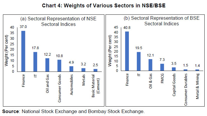

Table 1 provides a brief description of summary statistics of Brent crude oil prices and sectoral Indian stock indices returns. Brent shows negative mean returns while the returns for all 10 stock sectors are positive for the selected period of 3632 days. But the median for all series (including Brent) is positive.

Mean returns differ across different stock sectors with relatively higher returns for Consumer Durables, FMCG, and Financial Services sectors. The minimum and maximum values indicate Brent has the largest range of variation among all series. Further, the measure of standard deviation which is a primary measure of volatility indicates that the volatility of crude oil was the highest. Amongst stock indices, volatility was the highest for Metals followed by Financial Services and Oil and Gas sector. All series are negatively skewed (except the Capital goods sector) indicating a larger frequency of occurrence of negative returns than positive returns.

Furthermore, all the series are leptokurtic (heavier tails) indicating a higher probability of extreme returns. Negative skewness of nine sectors and very high positive kurtosis of all sectors indicate the non-normality of distributions. Moreover, the higher values of the Jarque-Bera³ test statistic confirm the non-normality of distributions.

III.2 Methodology

The choice of multinomial logit (MNL) framework is dictated by the flexibility embedded in the model. The framework enables the determination of the probability of excessive volatility in returns, termed exceedances in literature, occurring in global crude oil price and India’s stock price index at the aggregate as well as disaggregated sectoral levels. Also, the model allows for the incorporation of controls that might have contemporaneous effects on Indian sectoral stocks.

The most challenging part of the MNL framework is estimating threshold level of returns required as a precondition. The Extreme Value Theory (EVT) used to identify centre and tails – positive and negative, of any distribution comes in handy in estimating the centres and tails of the returns in global crude oil price changes and sectoral Indian stocks. It is only when the threshold level of return that distinguishes normal returns from extreme returns (positive or negative) is determined that one can proceed with the estimation process.

By using the method of historical simulation, the estimate of F(u) equals (n-N/n), where n is the sample size.

III.3 The Multinomial Logit (MNL) Model

Instances of co-exceedances point to cross-market or sectoral linkages. To analyse the cross-market or sectoral linkages, co-exceedances are further classified into different categories (m categories). As the explained variable is a qualitative variable, a multinomial logit model could be used to investigate the existence of contagion from the crude oil market to the Indian stock sectors. Logit models support categorical data and provide the probability of success of an event. The MNL model can be used to analyse the category of co-exceedances. If P (Y = i) be the probability associated with a category i of m possible categories, the MNL is given by

The coefficients of logit models are nothing but the marginal change in the probability of a unit change in the independent variables to test whether this change is statistically significantly different from zero,

IV. Empirical Analysis

IV.1 Threshold/Cut-off

As noted earlier, an appropriate threshold u is of utmost importance for estimation. A very high threshold (fewer observations) may help to reduce the bias but result in a large variance of parameter estimates, while a very low threshold (more observations) may make the estimates more efficient but may imply more values around the centre of the distribution. The thumb rule for estimating optimal threshold using Empirical Mean Excess Function (EMEF) method - the EMEF statistics should be linear in the best threshold ս₀. In other words, if the slope of the EMEF approximation is constant when u exceeds a certain level ս₀, then the optimal threshold is em > ս₀.

Threshold returns are reported in Table 2 using mean excess plots and an eyeball inspection approach. Two thresholds have been calculated for each stock sector and global crude oil price, respectively – one for the top tail of the distribution and the other for bottom tail. Those cases where returns are above the respective thresholds - top and bottom tails, are classified as positive exceedances, and those below the respective thresholds are classified as negative exceedances. The cases of simultaneous exceedances in more than one sector a day are called co-exceedances. There have been significant differences between optimal threshold levels of crude oil and stock sectors ranging from 2.02 per cent to 3.98 per cent for top tails and from -1.77 per cent to -3.78 per cent for bottom tails. The shape parameters (α) for all variables have been close to zero implying that the residuals are characterised by Pareto distribution along both the tails. Both scale (ψ) and shape parameters (α) or tail index (ξ) of the GPD function for top and bottom tails are also provided in Table 2.

A comparison of the threshold levels for both top and bottom tails would show that no stock sector in India registered volatility in returns as high as that registered by global crude oi price during the period considered. Significant variations were also observed as regard exceedances within the stock sectors. Stock sectors like Auto, Basic Materials, Capital Goods, Commodities and Consumer Durables registered higher negative exceedances compared with sectors like Financial Services, FMCG, IT, Metal and Oil and Gas Sectors. The Maximum Likelihood Method is used to estimate the shape and scale parameters.

IV.2 Exceedances and Co-exceedances

As mentioned already, the determination of threshold volatility/returns is the distinctive feature of the paper. As per standard practice in volatility analyses using MNL, exceedance or extreme volatility/return is defined as the ones that lie above or below the threshold levels, called positive or negative exceedances. On the other hand, co-exceedance is said to have happened when exceedance occurred in more than two sectors on the same day.

Not only had the number of days of co-exceedances for the respective groups been counted, but also the sectors that experience exceedances and how often they occur during the sample period. Based on frequency, co-exceedances (positive/ negative) have been categorised into five categories (Table 3: a and b). Of the 3632 trading days of the sample period, there were 706 days when positive contemporaneous exceedances were observed among the stock sectors as against 609 days of negative contemporaneous exceedances. At least two (2) sectors registered positive co-exceedances on 461 days as depicted in Group 2 and negative co-exceedances on 399 days (Table 3: a-b; Chart 5: a-b). This is indicative of the dominance of positive exceedances in sectoral returns. Basic Materials and Commodities sectors realised higher positive co-exceedances across all groups closely followed by Capital Goods, Financial Services, Metals, Automobiles, and Oil and Gas sectors compared with relatively lower positive co-exceedances for Consumer Durables, FMCGs, and IT stocks.

While the relatively low positive co-exceedances of the IT sector may be attributed to the sector’s relatively lesser volatile returns. This in turn can also be attributed to the relatively less prospect of profits for the sector being affected by volatility in global crude oil prices. The negligible input ratio for crude oil in the IT sector and its maturity in terms of competitiveness, size, stature, and as a brand with global reckoning further corroborate this observation. In fact, the sector has outperformed other sectors during periods of crisis such as pandemics.

As regards both FMCG and Consumer durables, their relatively fewer positive co-exceedances can be attributed to the dynamics of demand and supply, sensitive to preference but relatively stable in the short run, hence more credible and less volatile for the investor. For the negative co-exceedances, though there was no sector that dominated all the groups, sectors like Financial Services, Metals, Commodities, and Basic Metals registered higher co-exceedances compared to sectors like IT, Oil, and Gas, FMCGs, Consumer Durables, Automobiles, and Capital Goods. Broadly, sectors that registered higher positive co-exceedances were also sectors that registered lower negative co-exceedances.

However, there has been an asymmetry with Basic Metals, Commodities, and Metal registering high negative as well as positive co-exceedances and relatively low but stable distribution for the Oil and Gas sector on both sides. For Basic Metals, Commodities and Metals, this can be gauged in terms of the cash flow and input costs channels from these sectors to other sectors, such as chemicals, petrochemicals, fertilisers, and cement.

As regards, Oil and Gas stock sector, instances of co-exceedances were lower than expected. Ideally, extreme volatility witnessed in international crude oil prices should have reflected in higher exceedances and co-exceedances in Indian Oil and Gas stock sector returns given India’s high dependency on imported crude oil and as petroleum products account for around 68 per cent of the input costs in Oil and Gas sector as per NAS-based industry classification input-output matrix of India. The relatively stable stock returns for Oil and Gas sector may be reflective of administrative price mechanism of oil and fuel during much of the period under study which may have not only impeded smoother pass-through of changes in global crude oil prices to domestic market with implications on the prospects of profit for oil marketing companies and the stock returns.⁴ It is worth noting that as the number of stock sectors considered are enlarged (Group 4/5, Table 3:a and b), the days of co-exceedances increased for both the tails. This may be reflective of the fact that petroleum products are used as inputs in various other ancillary sectors. The by-products of crude petroleum like petrol, diesel, kerosene, and other petrochemicals are also used as inputs in other industries like cement, fertiliser, chemicals, tyre and paints, among others. Petroleum products are also used in fertiliser industries up to 10 per cent as input, 4-7 per cent in chemical industries, and 7 per cent in cement industries.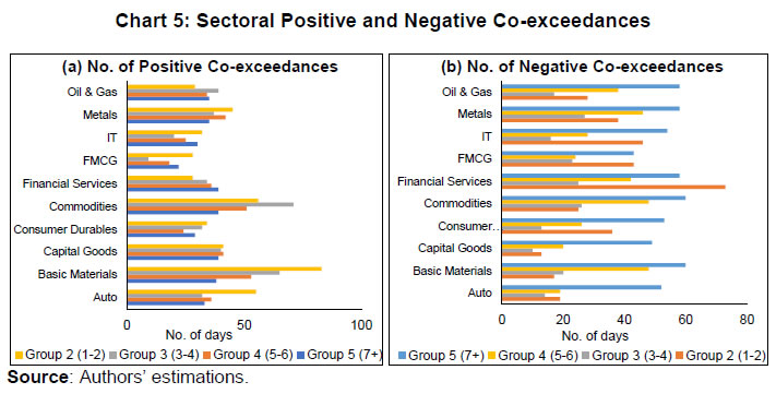

As it emerged, there was not a single stock sector that had not experienced co-exceedances during the period under study. Six (6) stock sectors are likely to experience more positive co-exceedances on any given day than negative co-exceedances while three stock sectors higher negative co-exceedances indicating asymmetry in the distribution. The occurrence of high co-exceedances – positive or negative, among the 10 stock sectors suggests that the 10 sectors form part of the tail of the distribution and that there exists a strong contagion within sectors.

IV.3 Regression Results of MNL

In the MNL framework, the coefficients are gauged assuming one of the categories as a base. The base category is assumed in turn to have no coefficient. Also, as in the previous section, the 10 sectors are classified into five groups depending on exceedances/co-exceedances, namely, base category, categories 1….4, respectively. The MNL model gives four coefficients for each covariate except the base category, denoted as βi1, βi2, βi3, βi4 where i denotes the covariate i, representing one or two sectors experiencing exceedances contemporaneously, three or four sectors, five or six sectors, and seven or more sectors, respectively. The estimated coefficients are gauged against the base category.

The two covariates so selected – by estimating top and bottom tails, for estimating contagion to Indian stock sectors from the crude oil market on which the MNL regression is run are oil price exceedances and oil price conditional volatility, respectively. As it emerged, for the positive co-exceedances, the regression coefficients on crude oil price exceedances were positive and statistically significant at levels ranging between 1 or 5 per cent for co-exceedances in all the 10 stock sectors categorised under Groups 1 to 5. This indicates that all the 10 stock sectors are likely to experience positive co-exceedances when faced with extreme positive returns in global oil markets. As against this, for negative co-exceedances, the coefficients are negative and significant for eight stock sectors, barring stock sectors in Group 3. The negative sign of the coefficients for negative co-exceedances indicates that in three or more stock sectors the probability of exceedances occurring simultaneously reduces when faced with extreme negative returns in oil markets. This is indicative of the dominance of positive co-exceedances in Indian stock sectors due to global crude oil returns exceedances. Likewise, the observation – higher the volatility of oil returns measured in terms of conditional variance, the higher is the probability of contemporaneous exceedances in three or more sectors, significant at 1 per cent level, are along expected line. These observed near total co-exceedances across all 10 stock sectors contemporaneous with crude oil returns exceedances – positive or negative, point to the existence of a strong contagion effect between global oil price exceedances and exceedances in Indian stock sectors (Table 4).

For enhancing the robustness, and to avoid endogeneity arising out of omission of relevant variables as the regression pertains only to oil-related variables, three variables affecting stock markets have been identified as controls. This approach is in line with the literature (Fang and Egan, 2018). These are returns on the INR-USD exchange rate, 10-Years G-Sec Yield, and Small Minus Big (SMB)⁵ difference in the yield for small and big firms.

The choice of these variables is driven by various factors. First, both foreign exchange and stock markets are highly volatile and are the most traded financial markets. Secondly, as per the ‘portfolio rebalancing approach’, the bond market also affects the returns in the stock market. Government bonds are risk-free but have lesser returns while stocks are risky but have higher returns. When government bond yield rises, it may impact stock market as higher bond yield would attract more investment. Thirdly, the small minus big (SMB) model is an important stock pricing model, according to which if a portfolio has more small-cap companies in it, it should outperform the market over the long run.

As expected, after incorporating these three control variables, the Pseudo R² improved significantly from 0.033 to 0.1 for positive co-exceedances, and from 0.052 to 0.12 for negative co-exceedances pointing that these factors also wield an impact on sector co-exceedances. Further, with these control variables, the predictive power of exceedances of covariance for oil returns for stock sectors co-exceedances improved for categories 3-4 for positive co-exceedances and categories 1-4 for negative co-exceedances (Table 5).

This observed tendency for co-exceedances among sectoral stock indices with exceedances in oil returns and the control variables, reinforced by the significance of log-likelihood tests for positive and negative co-exceedances, confirms the existence of contagion effect to Indian stock sectors not only from global oil returns and their conditional volatility but also from the control variables introduced. These observations also indicate that for India, the financial attribute of crude oil is significant and operating. The estimated coefficients on INR-USD exchange rate exceedances were the highest. This points to higher contagion effects from extreme fluctuations in INR-USD exchange rate to India stock sectors compared with global crude oil returns reflecting the dynamic reality of Indian economy i.e., more than 80 per cent of India’s exports and imports are invoiced in USD while more than 80 per cent of India’s consumption demand for fuel is met through imports. It is but also natural to expect that extreme movements in the benchmark 10-year G-sec yield - the channel for integration of various segments of the domestic financial market and the link between domestic and external financial markets, would have an impact on Indian stock markets, as also, the operation of yield differential between small and big firms as propounded by the SMB model for a financial market like India that has become fairly large and integrated with the global financial system.

In fact, the contagion effects of crude oil exceedances extend beyond the financial sector to real and macro-economic variables. According to an estimate by the Reserve Bank of India (RBI, 2022), at 10 per cent above the baseline of USD 100 per barrel for global crude oil price, domestic inflation and growth in India could be higher by around 30 bps and weaker by around 20 bps, respectively.

V. Conclusions

While most studies till now have focused on examining the relationship between global crude oil prices and macro-economic variables, this paper attempts to measure the contagion impact of extreme changes in global crude oil prices on 10 composite sectoral indices of the Indian stock markets.

The paper used generalised Pareto distribution to distinguish normal return from excessive returns by determining threshold returns, and in turn, positive and negative excess returns, namely exceedances. The probability of return exceedances contemporaneously occurring in these 10 sectoral indices along with exceedances in the Brent returns was tested using a multinomial logit framework.

The paper found strong statistical evidence of the likelihood of contagion effects from extreme changes in global crude oil price getting transmitted to sectoral indices of Indian stock markets. Of the two oil exceedances – positive and negative, the contagion effect of positive oil exceedances was not only dominating as indicated by the higher magnitude of the positive coefficients but was seen impacting all 10 sectoral stock indices compared with seven in the case of negative oil exceedances. The findings of the paper suggested that there might be other factors prompting a higher and more pervasive contagion on the sectoral stocks in the Indian market, the case in point being the INR/USD market.

The paper used a non-time varying threshold. Using a time-varying threshold may be an improvement as it would capture the fast-changing dynamics of the global as well as domestic financial and commodity markets; an issue that can be explored in the future work on this subject. Also, the paper examined the asymmetric aspect of the contagion effect on sectoral indices only partially. Notwithstanding these limitations, the paper underscores the contagion impact of extreme changes in global crude oil price on Indian sectoral stock indices in a pervasive manner. It also indicates the need for investors in Indian stock markets to hedge their portfolios as a mere diversification of portfolios may not be sufficient to protect their assets from an adverse oil price shock. Also, given India’s import dependence on crude oil and the observed co-exceedances, any negative stock may lead to a decline in market capitalisation and loss of wealth for investors.

Thus, the need for oil proofing the Indian economy – its financial and real sectors, from shocks or adverse geopolitical events cannot be overstated. This also points to the need for a policy for promoting energy security and sustainability. This calls for rapid investments in other alternative energy sources for which India has the potential of being self-sustainable. It would also be prudent on the part of regulators to be vigilant of the potential contagion from global crude oil price movements given their wider implications for systemic financial stability.

^@ Madhuchhanda Sahoo (msahoo@rbi.org.in) is Manager in the Department of Economic and Policy Research, Reserve Bank of India (DEPR), RBI and Arvind Kumar Shrivastava (arvindkshrivastava@rbi.org.in) is Assistant Adviser in Department of Statistics and Information Management (DSIM), RBI. Jessica Maria Anthony (jessicaanthony@rbi.org.in) is Assistant Adviser and Thangzason Sonna (tsonna@rbi.org.in) is Director in DEPR, RBI.

¹ Authors are grateful to Dr. Jugnu Ansari, Dr. Rajeev Jain and Edwin A. Prabhu for their valuable feedback. The views expressed in this paper are those of the authors and do not represent the views of the institution they are affiliated with.

² Input-output coefficients indicate the unit of petroleum products in value terms used as input to produce one unit of output in the respective sector. The coefficients are calculated using the input-output matrix for India for the BSE listed companies. Since the coefficients pertain to BSE listed companies, they are not comparable strictly with the input-output coefficients derived using National Accounts Statistics (NAS) sectoral classification.

⁴ The use of time-varying threshold framework is expected to help better capture exceedances and co-exceedances, especially for Oil and Gas stock sector since oil and fuel price deregulation has been affected more expeditiously in recent years.

⁵ SMB is a factor in the Fama/French stock pricing model according to which smaller companies outperform larger ones over the long-term. SMB is calculated as the difference in annual returns of BSE Large cap and Small cap companies.

References

Agren, M. (2006). Does Oil Price Uncertainty Transmit to Stock Markets?. Uppsala Universitet, Working Paper.

Aloui, R., Hmmoudeh, S. and Nguyen, D. K. (2013). A time-varying copula approach to oil and stock market dependence: The case of transition economies. Energy Economics, 39, 208–221.

Anand, B., Paul, S. and Ramachandran, M. (2014). Volatility spillover between oil and stock market returns. Journal of International Money and Finance, 30 (7),1387-1405. Retrieved from: https://www.sciencedirect.com/science/journal/02615606/30/7

Anand, B. and Paul, S. (2021). Oil Shocks and Stock Market: Revisiting the dynamics. Energy Economics, 96, 105111. Retrieved from https://www.sciencedirect.com/science/journal/01409883/96/supp/C

Arouri, M.E.H. (2011). Does Crude Oil Move Stock Markets in Europe? A Sector Investigation. Economic Modelling, 28(4), 1716-1725.

Asteriou, D., Dimitras A., and Lendewig A. (2013). The Influence of Oil Prices on stock Market Returns: Empirical Evidence from Oil Exporting and Oil Importing Countries. International Journal of Business and Management, 8(18), 101-120.

Bastianin, A., Manera, M. (2018). How Does Stock Market Volatility React to Oil Price Shocks? Macroeconomic Dynamics, 22 (3), 666-682.

Bhar, R., Nikolova, B. (2009). Oil Prices and Equity Returns in the BRIC Countries. World Economy, 32(7), 1036-1054.

Chan-Lau, J. A., Mitra, S. and Ong, L. L. (2012). Identifying Contagion Risk in the International Banking System: An Extreme Value Theory Approach. International Journal of Finance and Economics, 17(4).

Cheikh, N. B., Naceur, S. B., Kanaan, O., and Rault, C. (2018). Oil Prices and GCC Stock Markets: New Evidence from Smooth Transition Models. IMF Working Paper, 18(98).

Chittedi, K. R. (2012). Do Oil Prices Matters for Indian Stock Markets? An Empirical Analysis. Journal of Applied Economics and Business Research, 2(1), 2-10.

Cunado, J. and Gracia F. P. (2005). Oil prices, Economic Activity and Inflation: Evidence for Some Asian Countries. The Quarterly Review of Economics and Finance, 45(1), 65-83. Retrieved from: https://econpapers.repec.org/article/eeequaeco/

Degiannakis, S. A., George, F. and Arora, V. (2018). Oil Prices and Stock Markets: A Review of the Theory and Empirical Evidence. The Energy Journal, 39 (1).

Degiannakis, S., Filis G. and Arora, V. (2017). Oil Prices and Stock Markets. www.eia.gov.

Degiannakis, S., Filis G. and Floros C. (2013). Oil and stock price returns: Evidence from European industrial sector indices in a time-varying environment. Journal of International Financial Markets Institutions and Money, 26 (C), 175-191.

Fang, S. and Egan, P. (2018). Measuring Contagion Effects Between Crude Oil and Chinese Stock Market Sectors. The Quarterly Review of Economics and Finance,68(C), 31-38. https://ideas.repec.org/a/eee/quaeco/v68y2018icp31-38.html

Ghosh, S. and Kanjilal. K. (2016). Co-movement of international crude oil price and Indian stock market: Evidences from nonlinear cointegration tests. Energy Economics, 53, 111–117.

Gomes, M. and Chaibi, F. A. (2014). Markets, Volatility Spillovers Between Oil Prices And Stock Returns: A Focus On Frontier. The Journal of Applied Business Research, 30(2), 509-526.

Hamilton, J. D. (1983). Oil and the Macroeconomy since World War II, Journal of Political Economy, 91(2). 228-248.

Hamilton, J. D. (2003). What is an Oil Shock? Journal of Econometrics, 113, 363-398.

IEA (2019), Oil Market Report 2019, IEA, Paris, https://www.iea.org/topics/oil-market-report.

Imarhiagbe, S. (2010). Impact of Oil Prices on Stock Markets: Empirical evidence from Selected Major Oil Producing and Consuming countries. Global Journal of Finance and Banking Issues, 4(4).

Jambotkar, M. and Anjana, R. G. (2018). Impact of Macro Economic Variables on the Selected Indian Sectoral Indices: An Empirical Analysis, International Journal of Academic Research and Development, 3(2), 450-456.

Kang, W., de Gracia, F. P., and Ratti, R. A. (2017). Oil Price Shocks, Policy Uncertainty, and Stock Returns of Oil and Gas Corporations. Journal of International Money and Finance, 70, 344-359.

Kilian, L. and Park, C. (2009). The Impact of Oil Price Shocks on the US Stock Market. International Economic Review, 50 (4), 1267–1287.

Makhija, H. and Raghukumari, P.S. A Study on Impact of Oil Prices on Emerging Market Stock Indices. Journal of Economics and Finance, 35-40.

Monetary Policy Report (RBI, April 2022). External Environment, Chapter V.https://www.rbi.org.in/Scripts/PublicationsView.aspx?id=21023#CH5

Narayan, P. K. and Sharma, S. S. (2011). New Evidence on Oil Price and Firm Returns. Journal of Banking and Finance, 35(12), 3253-3262.

Rai, V. P. and Bairagi, P. (2014). Impact of changes in Oil Price on Indian Stock Markets. ResearchGate.

Rajan, A. P. and Lourthuraj, S. A. (2020). Financial Analytics: Time Series Analysis Impact of Crude Oil Prices on Automotive Stock. International Journal of Scientific and Technology Research, 9(3).

Ratti, J. I. M. and Ronald, A. (2009). Crude Oil and Stock Markets: Stability, Instability, and Bubbles. Energy Economics, 31(4), 559-568.

Salgado, R.J.S., Villarreal, C. C. and Martínez, F. V. (2017). Impact of Oil Prices on Stock Markets in Major Latin American Countries (2000-2015). International Journal of Energy Economics and Policy, 7(4), 205-215.

Sathyanarayana, S., Harish, S. N. and Gargesha. S. (2018). Volatility in Crude Oil Prices and its Impact on Indian Stock Market Evidence from BSE Sensex. Journal of Management, 9(1), 65-76.

Singhal, S. and Ghosh, S. (2016). Returns and volatility linkages between international crude oil price, metal and other stock indices in India: Evidence from VAR-DCC-GARCH models. Resources Policy. 50 (C), 276-288.

Teulon, F. and Guesmi, K. (2014). Dynamic Spillover Between The Oil And Stock Markets of Emerging Oil-Exporting Countries. The Journal of Applied Business Research, 30(1).

Thorbecke, W. (2019). Oil Prices and the U.S. Economy: Evidence from the Stock Market. RIETI Discussion Paper Series.

Youssef, M. and Khaled, M. (2019). Do Crude Oil Prices Drive the Relationship between Stock Markets of Oil-Importing and Oil-Exporting Countries? Economies, 7(3), 70.