Press Release RBI Working Paper Series No. 12
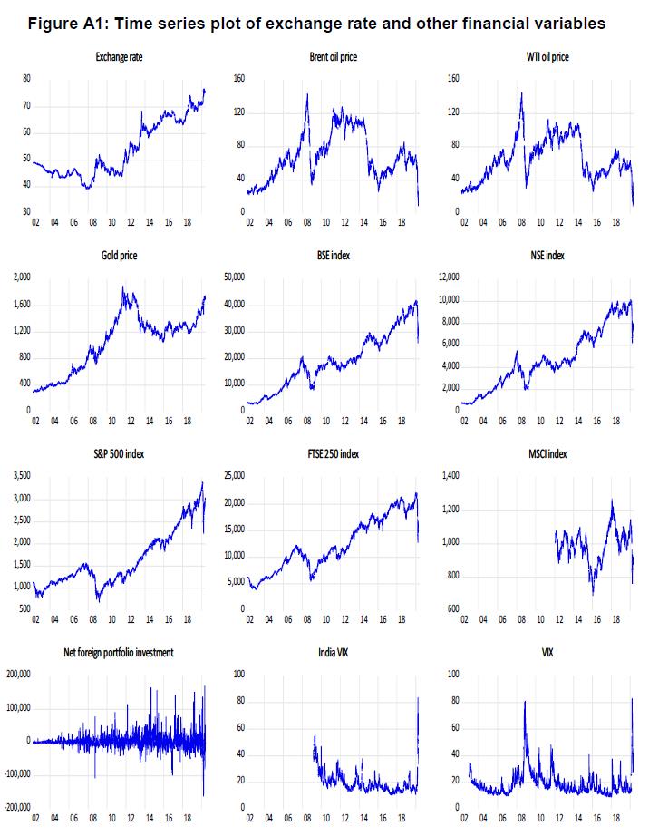
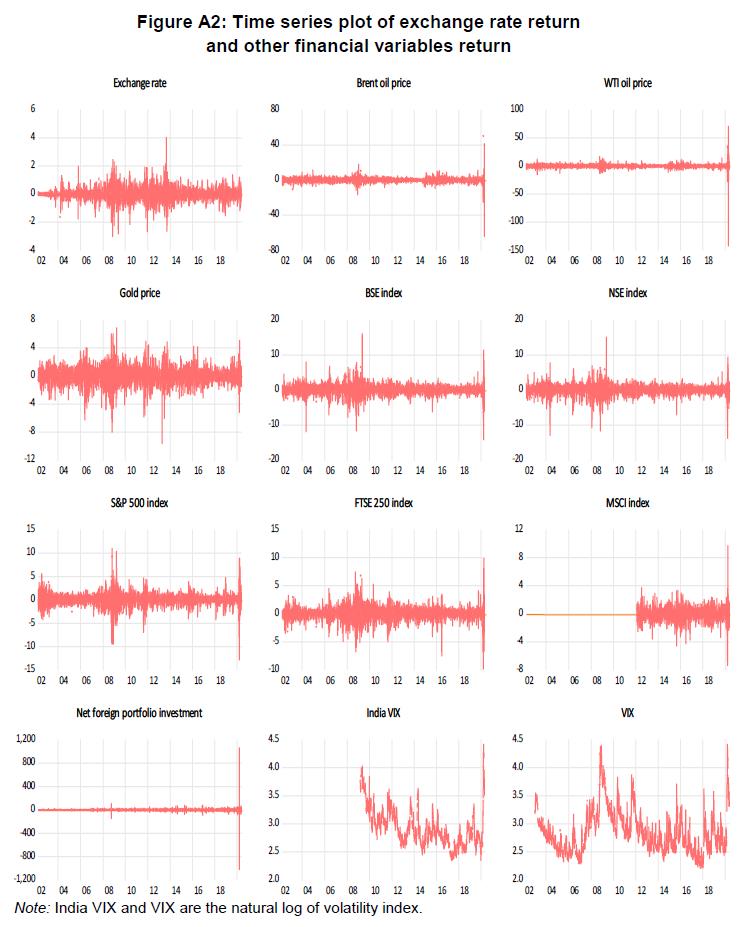
Predicting Exchange Rate in India: A Non-parametric Causality-in-Quantiles Approach Seema Jaiswal@ Abstract 1Financial asset prices are widely used for predicting exchange rate movements. This paper examines the relationship between the INR/USD exchange rate and select commodity market and stock market variables using a non-parametric causality-in-quantiles approach. The paper finds that changes in crude oil, gold, stock prices and VIX exhibit causality with the exchange rate for all quantiles barring the two extreme ends of the conditional distribution. The causal relationship of the West Texas Intermediate (WTI) oil price, domestic and global stock indices and gold price with the exchange rate of the INR/USD is stronger in mean than in variance, while it is stronger in variance for the Brent crude oil price and net foreign portfolio flows. JEL classification: C32, F31, G10, Q02 Keywords: Exchange rate, commodity price, stock price, volatility, quantile causality Introduction The impact of volatility in domestic and international asset prices on the exchange rate of the Indian Rupee (INR) has increased considerably over time due to greater financial and trade integration. Excessive exchange rate volatility for an extended period may have a negative effect on many economic indicators and pose significant financial stability risks (RBI, 2022). The aim of this paper is to study the causal linkages of domestic and global market indicators with the exchange rate of INR, using the non-parametric causality-in-quantiles technique. There is a vast literature on the determinants of exchange rate and econometric techniques that could help to predict the exchange rate. The early literature focused on studying the short- and long-run relationships between these variables using Granger causality, cointegration and error correction techniques. Some studies empirically tested the time-varying co-movements and dynamic volatility spillover impact of various macro-economic variables on the exchange rate using various formations of GARCH (Generalised AutoRegressive Conditional Heteroskedasticity) modelling. There are also recent studies providing evidence on the inter-dependencies among these variables and the exchange rate using the wavelet multi-resolution analysis. The linkages between the macro-economic and financial variables on the one hand, and the exchange rate on the other as captured through the aforementioned approaches are based on the conditional mean distribution of the exchange rate. The results based on conditional mean analysis may be ambiguous, especially when the distribution of a given variable is fat-tailed, as is the case with daily exchange rate returns. Thus, the conditional mean-based method may not delineate the complete causal relationship between two variables. To address such methodological limitations, the present study uses the conditional quantile method that captures the linkage of one variable with another under various foreign exchange market conditions2 i.e., across different quantiles of the exchange rate. The study is based on a long-time series data spanning April 2002 to May 2020, with daily frequency as against monthly, quarterly or annual data typically used in other studies, facilitating a deeper study of the dynamics of the exchange rate changes. The study examines the pairwise causal relationship between exchange rate return and a comprehensive set of macro-economic and financial variables using a non-parametric causality-in-quantiles technique recently developed by Balcilar et al. (2017a).3 This is the first study to the best of our knowledge that examines the causality of exchange rate using a comprehensive set of market indicators and daily data for India. The present study makes useful contributions to the existing literature. First, the non-parametric causality-in-quantiles approach helps in - (i) identifying dependencies for higher order (causality in variance) as there can be weak causality in return (mean) among financial variables but there can be significant causality in variance, due to volatility spillovers; (ii) exploring the dependence structure using a nonparametric procedure, that reduces the probabilities of mis-specification errors, (iii) studying non-linear time series having structural breaks, as most of the financial variables (especially with daily frequency) are non-linear. In fact, all variables used in this study are found to be non-linearly related to the exchange rate. Further, it helps to find the presence of causality at each point of the respective conditional distributions during the period of low fluctuations (the lower quantiles), normal fluctuations (median), and high fluctuations (the upper quantiles) of exchange rate return and volatility. This is also important when the dependent variable has fat-tails, as is the case with exchange rate return. The rest of the study is organised as follows: Section 2 presents the literature review, Section 3 discusses data and methodology, and Section 4 provides the empirical findings. Finally, Section 5 concludes. 2. Literature Review Since March 1993, the exchange rate regime of India can be deemed as market-determined with no fixed target (Jalan, 2000). As per the International Monetary Fund‘s (IMF) classification of exchange rate regimes of member countries as specified in the Annual Report on Exchange Rate Arrangements and Exchange Restrictions (AREAR), India follows a flexible exchange rate regime. The movement of the exchange rate is determined by the demand and supply dynamics of the US dollar (USD) in India, which in turn is influenced by several macroeconomic factors such as the trade balance, current account balance, net capital flows, movements in major global currencies, domestic and global political and economic developments, market expectations of relative interest rates and relative inflation for the INR and USD. The Reserve Bank intervenes intermittently, to maintain orderly market conditions by containing excessive volatility in the exchange rate (BIS, 2013). Pattanaik and Sahoo (2003) investigated the effect of RBI intervention on exchange rate and found that the intervention is effective in achieving the stated objective of policy. The Indian foreign exchange market has undergone significant changes with improved institutional and market infrastructure, a wide range of instruments and a more liberal regulatory structure. As per the Bank of International Settlements triennial survey of turnover in the foreign exchange market (2019), over-the-counter trades in the Indian rupee constituted 1.7 per cent of the total USD 6.6 trillion global foreign exchange market (BIS, 2019). The turnover of the average daily USD-INR pair increased to USD 110 billion in April 2019 from USD 56 billion in April 2016. As a result of the calibrated and gradual opening of the capital account and other external sectors of the Indian economy, the forex market has become increasingly integrated with the rest of the world. This is reflected in the increased volume of capital flows and growing trade in the foreign exchange market. Consequent to all these developments, the INR/USD exchange rate has witnessed extended periods of calm followed by intermittent extreme volatility due to sharp fluctuations in capital flows. As noted earlier, several studies have been undertaken to analyse the interdependencies among the foreign currency market (exchange rate), the commodity market (oil and gold price), the stock market (domestic and global) and capital flows (foreign portfolio investment). As all these markets are closely integrated, fluctuations in any one can have a direct or indirect impact on the others. In this section, we briefly review the empirical studies conducted for examining the relation of the exchange rate with the above-mentioned financial variables. The relevance of each variable in determining exchange rate movements is mentioned along with the related literature. 2.1 Exchange Rate vs Oil Price The oil price has been referred to as a non-monetary factor of exchange rate movements in the literature. “For an oil-importing country, rise in the price of oil worsens the balance of payments and eventually leads to currency depreciation, while it generates the current account surplus for oil exporters” (Krugman,1983). In countries having large oil imports, a small increase in the real oil price can result in a rise in the price of tradable goods and may result in the depreciation of the domestic currency. Chen and Chen (2007) showed the presence of causality from oil price to the exchange rate for G7 countries. Based on Hiemstra and Jones (1994) nonlinear causality test, Bai and Rath (2019) found a unidirectional causality from oil price to exchange rate for two emerging economies, China and India. The results of Tiwari et al. (2013) using the wavelet multi-resolution technique showed no causal relationship between exchange rate and oil price at the lower time scales (high frequencies) but found the presence of causality at higher time scales (lower frequencies) for India. Ghosh (2011) and Mishra and Debasish (2017) investigated the linkages between oil price and exchange rate for India using GARCH and exponential GARCH (EGARCH) models, respectively. Their results showed that an upsurge in oil price results in a weakening of the Indian currency against US dollar. Studies based on linear and non-linear models indicated mixed results for causal relationship between exchange rate and oil price; however, they miss out to explain the linkages of oil price return at various states of exchange rate returns. Our study attempts to explain the existence of causality-in-mean as well as causality-in-variance from oil price to exchange rate over the entire conditional distribution. 2.2 Exchange Rate vs Gold Price The significance of gold as an alternate financial asset increases during a period of uncertainty. After the global financial crisis, gold prices shot up considerably due to a surge in its demand all over the world. Various studies on determining the linkages between exchange rate and gold price focus on the role of gold as a hedge or safe haven. Capie and Wood (2005) found gold as a potential hedge against the USD and observed that US dollar exchange rates (sterling-dollar and yen-dollar exchange rates) are inversely associated with gold prices. Mark (2011), using dynamic conditional correlations for various USD-linked exchange rates, showed that gold is a weak safe haven and a strong hedge against the USD. Using cointegration and Granger causality tests, Apergis (2014) found the gold price as a strong predictor of the Australian dollar/US dollar exchange rate. Reboredo and Rivera-Castro (2014) showed the existence of a positive relation between gold price and USD depreciation for a varied set of currencies at all time scales using the wavelet multi-resolution analysis. Wang and Lee (2011) investigated the role of gold as a hedge against the yen and their results showed that it depends on the extent of fall in yen. Balcilar et al. (2017b) used causality-in-quantiles technique to test bi-directional causality between exchange rate and gold price for gold-producing countries. The results suggest that gold price return causes exchange rate return as well as exchange rate volatility, while only exchange rate return causes gold price volatility for most of the countries used in the study. Our study, using the causality-in-quantile, explains the relationship of gold price return with respect to exchange rate return under different market conditions while other studies on exchange rate return specific to India are based on empirical analysis based on the conditional mean. 2.3 Exchange Rate vs Stock Price Forex and stock markets are among the highly liquid financial markets globally. The interdependency between these two markets has increased over time due to the increase in capital flow and internationalisation of stock markets. Studying linkages between these markets may help to predict interconnectedness and volatility transmission between them. Numerous studies confirm linkages between stock and forex markets in the literature. Chien-Hsiu Lin (2012) found that the co-movements between exchange rates and stock prices are more robust during a crisis period than a normal period in emerging Asian markets. Cristiana and Carmen (2012) also found causality between these two variables in their study for selected developed and emerging financial markets. Malarvizhi and Jaya (2012) examined the co-movement between exchange rate and Indian stock market return and found the presence of bidirectional causality between the two variables. Reboredo et al. (2016) examined the dependence between the exchange rate and the stock price for emerging economies at extreme points using copula functions. The results of this study indicate the existence of asymmetric downside and upside spillover effects from one market to the other. Mitra (2017) found evidence of bidirectional volatility spillover and long-term relationship between stock price and the exchange rate using GARCH model. Simona et al. (2019) explored the co-movements between foreign exchange and the stock market by applying a dynamic conditional correlation mixed data sampling (DCC-MIDAS) model. Their results suggested the presence of higher conditional correlations during certain crisis episodes between the two markets. Kalra’s (2011) study found that an increase in the global volatility index (VIX) results in the depreciation of east Asia currencies. The methodology based on causality-in-quantile is more general in the sense that it detects the presence or absence of causality from domestic and global stock markets to exchange rate markets under various heterogenous market conditions of the exchange rate, thus supplementing the literature further, while other studies based on conditional mean are not able to ascertain the same. 2.4 Exchange Rate vs Multiple Financial Variables Various studies have explored the co-movements and interlinkages among these financial variables using their return and volatility. Samanta and Zadeh (2012) examined interlinkages among gold price, oil price, exchange rate and stock market returns using spillover indices. The findings of the study suggested the existence of a long-run relationship between these markets. Ciner et al. (2013) examined the relationship of stock, bond, gold and oil prices with exchange rate using a dynamic conditional correlation analysis and quantile regression based on the daily data of the US and the UK. Their results indicated that gold acts as a hedge against the exchange rate and bond market for the equity. Further, their results based on quantile regression suggested that gold consistently plays the role of a safe haven when the exchange rates fall significantly. Jain and Biswal (2016) for their study on India based on DCC-GARCH method inspected the relationship between the global price of gold, crude oil, exchange rate, and the stock market. Their results suggested a fall in gold price or crude oil price causes a weakening of the exchange rate and the stock price index. Atul et al. (2015) found the existence of one-way causality from gold prices to both stock prices and exchange rate using daily data for India. Mollick and Sakaki (2019) examined the relationship of select major currencies with respect to the USD, international oil price and world equity returns using a vector autoregression (VAR) method. Their study proposed that commodity currencies appreciate subsequent to positive oil price shocks and safe-haven currencies weaken with positive global equity shocks. Against the backdrop of the literature discussed above, the present study investigates the predictability of exchange rate return and volatility using select financial variables. There can be diverse interlinkages between the financial variables and exchange rate under different degrees of exchange rate movements. The causality-in-quantile helps to measure the causality for each point of the conditional distribution of exchange rate return and volatility. The study is important to fill the gap in the existing literature by finding the financial indicators causing exchange rate movements specific to India and providing useful insights to portfolio managers. 3. Data and Methodology 3.1 Data Daily data from April 2, 2002 to May 29, 2020 (excluding weekends and holidays), constituting 4,395 observations are used for analysis. High frequency data capture more dynamics of the financial time series data which are typically quite volatile. The study period covers various phases of exchange rate fluctuations including the global financial crisis of 2008-09. However, the selected period for some variables varies as per data availability. These variables are: India VIX (expected stock market volatility index calculated using the NIFTY Index option prices), VIX (expected stock market volatility index calculated using S&P 500 index option prices) and MSCI emerging markets index [Morgan Stanley Capital International index, an indicator to assess equity market performance in emerging markets]. Exchange rate (INR/USD), closing prices of stock indices of BSE, NSE, US S&P 500 index, UK FTSE 250 index and net portfolio investment flows (in rupees million) are sourced from the CEIC database. The gold price (per ounce) is taken from the World Gold Council and is denominated in USD.4 The oil prices data used are the spot prices taken from the Energy Information Administration (EIA), US Department of Energy. Both WTI and Brent crude oil prices (Europe price at FOB) are in USD per barrel.5 Data for VIX, India VIX and MSCI emerging market index are taken from NSE and other relevant sources.6 We have calculated the returns of the variables by taking the first difference of their natural logarithm and then multiplying by 100. Net foreign portfolio investment data are adjusted for negative values before taking log difference as per the standard practice, i.e., by adding a constant positive number which makes the minimum number (negative) in the whole series to a small positive number. For all variables except VIX and India VIX return, the data are in natural logarithm form. The descriptive statistics of the data as per the required transformation of the data as discussed above are given in Appendix Table A1. The average of daily returns of all the variables is positive (negative for MSCI emerging market return), small as compared to standard deviation and close to zero showing the absence of any type of trend in the data. It is evident that the stock price return in India is higher as compared to the global stock price return in the US, the UK, and emerging markets. The volatility of these variables as represented by standard deviation shows that the exchange rate has lower variability as compared to return on stock and commodities prices. Oil price returns and stock indices returns, as mentioned in the literature, are some of the most volatile variables among all commodity prices. The skewness statistics of exchange rate return and net portfolio flows are positive and skewed to the right (more positive return than negative return), while it is negatively skewed for all other return variables. The kurtosis value for each variable is significantly higher than normal distribution indicating that the series is highly peaked and thus leptokurtic. This implies that returns have larger, thicker tails than the normal distribution which reveals the occurrence of extreme returns more frequently. The Jarque–Bera test statistics show that not all the variables are normally distributed. All the variables are tested for stationarity at the level and if they are not stationary when the first difference (log difference) is taken. All the variables except net FPI, VIX and India-VIX are found to be I(1). Net FPI, VIX and India-VIX are I(0). Since VIX and India-VIX are volatility indices, the analysis is done by taking the log transformation of these two series. As we are examining the pair-wise causality between two financial time series, we have used the return of net FPI even though it is stationary at the level. The dynamic behaviour of these variables are shown in Figures A1 and A2, depicting these series in actual and in return form, respectively. Figure A1 shows that all the commodity prices, stock prices and exchange rates have shown an upward trend in general. During the periods 2003-2008 and 2009-2011, the exchange rate recorded appreciation (downward movement) as a result of huge capital inflows in India. However, the exchange rate recorded a sharp depreciation during the periods of global uncertainties - the global financial crisis (2007-2009); post-announcement effects of quantitative easing programmes by the US Federal Reserve from May 23, 2013 to September 4, 2013 (Fed taper tantrum); and the recent COVID-19 pandemic (February 27, 2020 to May 29, 2020). Figure A2 shows that most of the series exhibit strong clustering behaviour and sharp movements during the heightened global uncertainties. We have used both international oil prices, Brent crude and WTI oil price in our study as Brent is the benchmark price in India while WTI is the international oil price. The stock indices of the US and the UK are taken as both the countries have significant cross-border transactions in terms of trade and foreign investments with India. Both BSE and NSE indices are used due to their varied compositions. We check for the existence of nonlinearity in the relationship between exchange rate return with the selected variables in the study by applying the BDS test developed by Brock, Dechert and Scheinkman (1996).7 The test is exercised on each residual of VAR(1) model of exchange rate return with selected variables and on the residuals obtained from the AR(1) model of exchange rate return. Table A2 presents the results of the BDS test which indicate rejection of the null hypothesis at various embedding dimensions (m). This proves statistically that there is a non-linear relationship between the exchange rate return and each selected variable. The results of linear Granger causality indicate all variables except MSCI return, net FPI and India VIX, significantly cause exchange rate (Table A3). However, any inference based on linear Granger causality results may lead to mis-specification errors as there exist non-linear relationships among the variables. We conduct the Bai and Perron (2003) test and find multiple structural breaks (the VAR(1) model of exchange rate return with selected variables and the residuals obtained from AR(1) model of exchange rate return, Table A4). The Bai and Perron test is based on a dynamic programming algorithm which optimises the exhaustive computational procedure for testing multiple breakpoints of global minimiser of squared residuals (SSR). This approach can allow for autocorrelation and heteroskedasticity in the time series. In the test, we employ quadratic spectral kernel-based HAC (heteroskedasticity-autocorrelation-consistent (HAC) correction) covariance estimation using pre-whitened residuals. The results detect two structural breaks in NSE and S&P 500 returns on September 11, 2008 and April 3, 2014, respectively. There is no break observed in the VAR(1) model of exchange rate return incorporating BSE return, Net FPI, India VIX and VIX. There are three structural breaks in the VAR(1) model with WTI and two breaks with Brent crude oil price. Most of the break dates are during the global financial crisis and the ensuing quantitative easing programmes by the Federal Reserve. The presence of non-linearity and structural breaks in the selected variables support the use of a nonparametric causality-in-quantile approach, as this test is robust to such mis-specifications. 3.2 Methodology We use the methodology developed by Balcilar et al. (2017a) for uncovering nonlinear causality through a hybrid approach using the methodology of Nishiyama et al. (2011) and Jeong et al. (2012). We represent the dependent variable exchange rate returns as yt and the independent variables (selected variables) as xt. Causality in quantile is the more general form of causality based on conditional quantile distribution derived, which allows to test the existence at each quantile (here, the conditional expectation function is changed to conditional quantile distribution, Granger causality in mean corresponding to median quantile). In particular, we want to test the causality-in-variance (volatility transmission), causality running from selected financial variables to the volatility of exchange rate returns, which may exist even if there is no causality in the mean (1st moment). Rejecting the kth moment causality does not infer rejection of mth moment causality when k < m. At the first stage, Nishiyama et al. (2011) nonparametric Granger quantile causality is applied. For describing the higher-order moments causality, yt is expressed as:
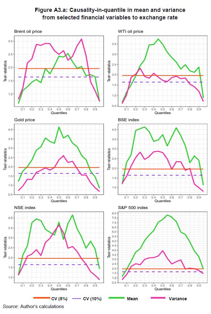
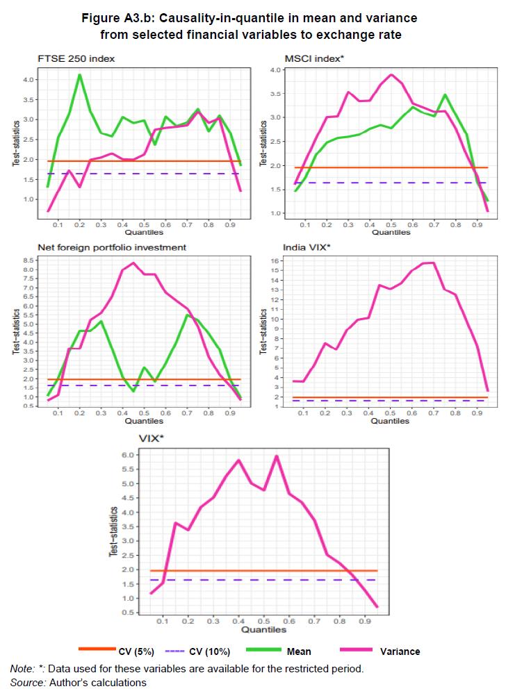
Consolidating the complete methodology, we specify that xnt Granger causes yt in quantile θ up to Kth moment based on equation (14), to build the test statistic of equation (6) for each k. It is not a simple exercise to combine different statistics for each k=1,2,…, K into a single statistic for the joint null specified in equation (14) as the statistics are mutually correlated (Nishiyama et al., 2011). Nishiyama et al. (2011) prescribe sequential-testing methodology with a few changes to tackle this problem. At the first stage, for the first moment (k = 1), the nonparametric Granger causality test is conducted. However, the rejection of the null hypothesis, i.e., the presence of non-causality does not imply that there does not exist causality in the second moment (k=2). At the next stage, we test the null hypothesis for k=2, causality in the second moment (variance) and hence, can test causality in mean and in variance successively. Therefore, for testing causality-in-quantiles, the empirical analysis requires defining three important parameters: the bandwidth h, the lag order p, and the kernel type for K (.) and L(.) in equation (6) and (9), respectively. The lag order, p=1 is selected based on the results of the Schwarz Information Criterion (SIC) for the VAR model of exchange rate return with other selected variables. SIC criteria is used because it helps to address the problem of over parametrisation that generally occurs in nonparametric techniques. The least squares cross-validation method is employed for choosing the bandwidth value and Gaussian-type kernels for K (.) and L(.) are applied. 4. Empirical Findings We now examine the results of the causality-in-quantile test, conducted for each selected variable and exchange rate, in mean (return) and in variance (squared returns, i.e., volatility). Figures A3.a and A3.b (Tables A5.a and A5.b) show the results of the above-stated tests. Various quantiles are shown along the horizontal axis and nonparametric causality test statistics are plotted against the vertical axis. The two horizontal lines refer to 5 per cent critical value of 1.96 and 10 per cent critical value of 1.65 respectively. The null hypothesis is non-existence of Granger causality (in mean and in variance) from the select variable to exchange rate. We have described the results by considering the rejection of the null hypothesis at 5 per cent level of significance. The analysis is presented in four categories: (i) International commodity prices (oil and gold), (ii) Domestic and global stock return, (iii) Net portfolio investment inflows, and (iv) Domestic and global volatility indices. International commodity prices: WTI oil price return (Figure A3.a) predicts exchange rate return over the quantile range of 0.25 to 0.90 while Brent oil return predicts over a shorter quantile range of 0.45 to 0.75. However, in variance, Brent crude oil price predicts exchange rate volatility over higher range (0.15 to 0.80) than WTI price (0.20, 0.25 and 0.40). This implies both WTI and Brent crude oil influence exchange rate barring extreme volatile periods. Most studies examining the linkages between oil price and exchange rate reveal the existence of causality and volatility spillover from oil price to exchange rate except a few, such as Tiwari et al. (2013), which based on wavelet analysis, found the presence of causality only at higher time scales (lower frequencies). In line with the literature, our results also confirm the existence of causality and volatility spillover from oil price return to exchange rate return and further show that it holds for a specific quantile range of exchange rate return. Gold price return predicts exchange rate return at all points except at lower and upper tail of its conditional distribution. Gold price return causes exchange rate volatility only around the median to moderately high quantiles (0.45 to 0.65). This implies gold serves as a hedge against the USD during the normal period and is in line with the findings of the study by Capie and Wood (2005). Domestic and global stock return: BSE index return predicts exchange rate for almost all quantiles except at tails (0.10 and 0.95) and similar results hold for NSE index return. For causality-in-variance, BSE return affects exchange rate covering quantiles around the conditional mean except at lower and upper quantiles (Figure A3.a). In terms of volatility, NSE return impacts the exchange rate for a relatively shorter-range (0.15 to 0.70) than BSE. The integration between stock price and exchange rate for India has been found in various studies as indicated in Section 2.3. There are limited studies focusing on the dependence structure of these two markets under extreme exchange rate market conditions. Our results are in line with Reboredo et al. (2016) who examined the downside and upside risk spillover between these two markets for emerging economies suggesting lower tail dependence and absence of upside spillover effects. The US stock market return (S&P 500), the UK stock market (FTSE 250) return and the emerging markets stock market return (MSCI) predict exchange rate return over the quantile range of 0.15 to 0.90, 0.10 to 0.90 and 0.15 to 0.85, respectively (Figures A3.a and A3.b). In terms of the impact of volatility from these global stock indices on exchange rate volatility, our results show that the US stock market and emerging stock market returns cause volatility in the exchange rate returns over most of the quantiles other than at extreme tails on both sides of the conditional distribution, i.e., barring periods of extreme low and high exchange rate volatility. The volatility in the UK stock (FTSE 250) exhibits nearly similar results as the other two global indices but does not have significant causalities at some lower quantiles. These results are consistent with the literature (Reboredo, 2016). The association between the exchange rate and stock price (as per stock-oriented model) states that a positive change in stock price of an economy encourages foreign investors in domestic markets, which in turn leads to high demand for local currency and results in an appreciation of the exchange rate. Any positive (negative) change in global stock market results in strengthening (weakening) of foreign currency. Domestic stock market and global stock market are closely integrated. Hence, the global stock market also indirectly impacts the exchange rate. As already noted, we have used the three major global stock indices, S&P 500 (the US stock market stock index), FTSE 250 (the UK stock index) and MSCI (the emerging market index) in the analysis. The results support the findings by Mollick and Sakaki (2019) which examined co-movements between 14 major currency/USD pairs with two global factors (oil and world equity returns). Net portfolio investment inflows: Net portfolio is measured as the difference between gross inflows and gross outflows of portfolio investments. Portfolio investment flows are among the most volatile component of capital flows, substantial variation in these flows may result in an appreciation or depreciation of the exchange rate. Net portfolio return predicts exchange rate return around the conditional mean covering quantiles range from 0.10 to 0.85 (Figure A3.b). An almost similar pattern is observed for causality in variance; however, the net portfolio prediction for exchange rate is stronger in variance than in mean. Domestic and global volatility index: We now consider the impact of the two volatility indicators, India VIX and VIX representing the near-term volatility of market expectations derived using NIFTY and S&P 500 index options, respectively. Both the volatility indices indirectly measure domestic and global uncertainty. The high value of these indices may result in wide fluctuations in other related markets, which in turn could impact the exchange rate. India VIX predicts exchange rate volatility over its entire conditional distribution (Figure A3.b). VIX predicts exchange rate volatility for the quantile range 0.15 to 0.80. The above results show that domestic India’s VIX impacts exchange rate volatility across all quantiles of the conditional distribution of exchange-rate volatility, while VIX does not significantly predict exchange rate volatility during periods of low and high volatility. It is also important to note that these two variables have the strongest predictive power for exchange rate volatility as compared to all other variables used in the study. The above results provide several important insights. The strength of causality of each variable with exchange rate return and volatility is asymmetric at different quantiles. Specific financial variables may have a causal relationship with exchange rate in mean but not in variance for a particular quantile. All the selected variables under consideration predict exchange rate return and volatility around the middle quantiles, i.e., during normal periods. 5. Conclusions The objective of the study is to assess the effect of international crude oil price, gold price, domestic and global stock price indices, net portfolio investment flows and volatility indicators on the quantiles of the conditional distribution of INR exchange rate return and volatility using daily data from April 2002 to May 2020. Non-linear interdependencies between the selected variables and exchange rate were examined using a non-parametric causality-in-quantiles test developed by Balcilar et al. (2017a). The method established the relationship between the two bivariate financial variables under all diverse conditions that can be categorised in the current study as bearish, normal and bullish phases of the foreign exchange market. The preliminary results of tests on non-linearity and structural break for exchange rate return’s relationship with the selected variables upheld the use of the non-linear causality-in-quantiles test. Evidently, the results of linear causality could not be relied upon. We found the presence of causality from the selected financial variables around the median of the conditional distribution of exchange rate return. This is in line with the findings of the empirical studies evidencing the causal relationship based on linear and various non-linear causality models. The results of causality-in-variance showed that Brent crude oil price, domestic and global stock index returns, net portfolio investment return and VIX significantly cause variations in the exchange rate return around the normal periods of exchange rate volatility i.e., not covering lower and upper quantiles. However, gold price returns predict exchange rate volatility from middle to upper quantiles and WTI oil price predicts for only a few lower quantiles. Studies based on the volatility spillover from stock prices to exchange rate show mixed results specifying the volatility spillover between them (Mitra, 2017) and additionally, the study by Mollick and Sakaki (2019) suggested that the spillover effect was greater from downside risk than the upward risk of the exchange rate. Our study also showed that the linkages between the exchange rate return and stock price varied at different points of conditional quantile distribution of the exchange rate. The existing studies based on conditional mean show the presence of causality from gold prices to exchange rate, but the studies based on the DCC-GRACH model show that gold can be considered as a potential hedge against exchange rate movements (Ciner et al., 2013; Aftab et al., 2019). Our study also indicated similar results as the dependency around the median quantile indirectly underlined the hedging role of these two markets under normal market conditions of the exchange rate. Both the indicators of market expectations of near-term volatility, VIX and India’s VIX had a strong power to predict exchange rate volatility. India’s VIX predicted exchange rate volatility over the entire conditional distribution of exchange rate volatility. The VIX as a global risk aversion indicator showed a limited role in explaining the exchange rate volatility as compared to India’s VIX may be due to a lower degree of financial openness. Overall, the causality-in-quantile approach helped in ascertaining the existence/ non-existence of causality relationship between select financial parameters (pairwise) and the exchange rate in mean and in variance at various quantiles. Of course, other than these variables, market intervention, capital account-based measures by the Reserve Bank and other administrative measures by the Government also played a role in controlling the extreme exchange rate movements. In sum, the study provided insights for policymakers, international investors, and hedge fund managers to ascertain the directional causalities from select financial variables to the exchange rate in various states of forex market. The analysis is also useful to determine how these selected asset classes (financial market and commodity) can be used to minimise exchange rate risk, especially during periods of extreme exchange rate volatility.
References Aftab, M. & Syed Zulfiqar Ali Shah & Izlin Ismail. (2019). Does Gold Act as a Hedge or a Safe Haven against Equity and Currency in Asia? Global Business Review, International Management Institute, vol. 20(1), pages 105-118. Apergis, N. (2014). Can gold prices forecast the Australian dollar movements? International Review of Economics and Finance, 29, (C), pp. 75-82. Bal, D. P. & Rath, B. N. (2019). Nonlinear causality between crude oil price and exchange rate: A comparative study of China and India - A Reassessment. Economics Bulletin, 39 (1). pp. 1-14. Bai, J. & Perron, P. (2003). Computation and Analysis of Multiple Structural Change Models. Journal of Applied Econometrics, 18(1), pp. 1–22. DOI: 10.1002/jae.659. Balcilar, M., Gupta, R., Kyei, C. & Wohar, M. E. (2016a). Does Economic Policy Uncertainty Predict Exchange Rate Returns and Volatility? Evidence from a Nonparametric Causality-in-Quantiles Test. Open Economies Review, Springer, vol. 27(2), pp. 229-250, April. Balcilar, M., Bekiros, S. & Gupta, R. (2017a). The role of news-based uncertainty indices in predicting oil markets: a hybrid nonparametric quantile causality method. Empirical Economics, issue 3. Balcilar, M., Gupta, R. & Pierdzioch, C. (2017b). On exchange-rate movements and gold-price fluctuations: evidence for gold-producing countries from a nonparametric causality-in-quantiles test. International Economics and Economic Policy, Springer, vol. 14(4), pp. 691-700, October. Bank for International Settlements (BIS) (2019). Triennial Central Bank Survey of Foreign Exchange and Over the counter (OTC) Derivatives Markets in 2019. BIS (2013). Market volatility and foreign exchange intervention in EMEs: what has changed? BIS Papers No. 73. Broock, W. A., Scheinkman, J. A., Dechert, W. D. & LeBaron, B. (1996). A test for independence based on the correlation dimension. Econometric Reviews 15(3), pp.197–235. Capie, F., Mills, T. C. & Wood, G. (2005). Gold as a hedge against the dollar. Journal of International Financial Markets, Institutions and Money 15, pp. 343-352. Chen, S. S. & Chen, H. C. (2007), Oil Prices and Real Exchange Rates. Energy Economics, 29, pp. 390–404. Ciner, C., Gurdgiev, C. & Lucey, B. M. (2013). Hedges and safe havens: An examination of stocks, bonds, gold, oil and exchange rates. Int. Rev. Financ. Anal. 2013, 29, pp. 202–211. Cristiana, T. & Carmen, P. D. (2012). On the Causal Relationship between Stock Returns and Exchange Rates Changes for 13 Developed and Emerging Markets. Procedia - Social and Behavioral Sciences, Volume 57, 2012, pp. 275-282. Das, D., Kumar, S. B., Tiwari, A. K., Shahbaz, M. & Hasim, H. M. (2018). On the Relationship of Gold, Crude Oil, Stocks with Financial Stress: A Causality-in-Quantiles Approach. Finance Research Letters (2018), doi: 10.1016/j.frl.2018.02.030. Dai, X., Wang, Q., Donglan, Z. & Zhou, D. (2020). Multi-scale dependence structure and risk contagion between oil, gold, and US exchange rate: A wavelet-based vine-copula approach. Energy Economics. 104774. 10.1016/j.eneco.2020.104774. Ghosh, S. (2011). Examining crude oil price-exchange rate nexus for India during the period of extreme oil price volatility. Appl. Energy 88, pp. 1886–1889. Grassberger, P. & Procaccia, I. (1983). Measuring the strangeness of strange attractors. Physica D: Nonlinear Phenomena, Volume 9, Issues 1–2, 1983, pp. 189-208, ISSN 0167-2789. https://doi.org/10.1016/0167-2789(83)90298-1. Hiemstra, C. & Jones, J. D. (1994). Testing for linear and nonlinear Granger causality in the stock price volume relation. Journal of finance. Finance 49, pp. 1639–1664. Jain, A. & Biswal, P. C. (2016). Dynamic linkages among oil price, gold price, exchange rate, and stock market in India. Resources Policy, 49, pp. 179-185. Kalra, S. (2011). Global Volatility and Forex Returns in East Asia. International Review of Finance, International Review of Finance Ltd., vol. 11(3), pp. 303-324. Jalan, Bimal (2000). Development and Management of Foreign Exchange Markets: A Central Banking Perspective. Lecture delivered at the 21st Asia pacific Congress on 1st December 2000 at New Delhi. Jaya, M. & Malarvizhi, K. (2012). An analytical study on the movement of NIFTY index and exchange rate. International Journal of Marketing and Technology 2: pp. 274-282. Jeong, K., Hardle, W.K. & Song, S. (2012). A Consistent Nonparametric Test for Causality in Quantile. Econometric Theory, Cambridge University Press, vol. 28(4), pp. 861-887, August. Krugman, P. (1983). Oil Shocks and Exchange Rate Dynamics. NBER Chapters, in: Exchange Rates and International Macroeconomics, pp. 259-284, National Bureau of Economic Research, Inc. Lin, C.H. (2012). The co-movement between exchange rates and stock prices in the Asian emerging markets. International Review of Economics and Finance, Elsevier, vol. 22(1), pp. 161-172. Mark, J. (2011). Gold and the US dollar: Hedge or haven? Finance Research Letters, Elsevier, vol. 8(3), pp. 120-131, September. Mishra, S. & Debasish, S. S. (2017). Analysis of Volatility Spillover between Oil Price and Exchange Rate in India: GARCH Approach (January 2, 2017). SSRN: http://dx.doi.org/10.2139/ssrn.2892670. Mitra, P. K. (2017). Dynamics of volatility spillover between the Indian stock market and foreign exchange market return. Academy of Accounting and Finance Studies Journal, 21(2): pp. 1-12. Moagăr-Poladian, S., Clichici, D. & Stanciu, C. V. (2019). The Comovement of Exchange Rates and Stock Markets in Central and Eastern Europe. Sustainability, MDPI, Open Access Journal, vol. 11(14), pp. 1-22, July. Mollick, A. V., and Sakaki, H. (2019), Exchange rates, oil prices and world stock returns. Resources Policy, 61, pp. 585-602. Nishiyama, Y., Hitomi, K., Kawasaki, Y. & Jeong, K. (2011). A consistent nonparametric test for nonlinear causality—specification in time series regression. Journal of Econometrics, Elsevier, vol. 165(1), pp. 112-127. Pattanaik, S. & Sahoo, S. (2003). The Effectiveness of Intervention in India: An Empirical Assessment. Reserve bank of India, Occasional Papers, Volume 22, p. 21. https://rbi.org.in/Scripts/PublicationsView.aspx?Id=5705. Raza, S. A., Shah, N. & Shahbaz, M. (2018). Does economic policy uncertainty influence gold prices? Evidence from a nonparametric causality-in-quantiles approach. Resources Policy, Elsevier, vol. 57(C), pp. 61-68. Reboredo, J. C. & Rivera-Castro, M. A. (2014). Gold and exchange rates: Downside risk and hedging at different investment horizons. International Review of Economics and Finance, 34, pp. 267- 279. Reboredo, J. C., Rivera-Castro, M. A. & Ugolini, A. (2016). Downside and upside risk spillovers between exchange rates and stock prices. Journal of Banking & Finance, Elsevier, vol. 62(C), pp. 76-96. https://doi.org/10.1016/j.jbankfin.2015.10.011. Reserve Bank of India (2022). Report on Currency and Finance(Chap. 4). Samanta, S. K. & Zadeh, A. H. M. (2012). Co-movements of oil, gold, the US Dollar, and stocks. Modern Economy, 3(1), pp.111–117. Shi, G. & Liu, X. (2020). Stock price fluctuation and the business cycle in the BRICS countries: A nonparametric quantiles causality approach. Finance Research Letters, Elsevier, vol. 33(C). Shiva, A. & Sethi, M. (2015). Understanding Dynamic Relationship among Gold Price, Exchange Rate and Stock Markets: Evidence in Indian Context. Global Business Review, International Management Institute, vol. 16(5_suppl), pp. 93-111, October. Tiwari, A. K., Dar, A. B. & Niyati, B. (2013). Oil price and exchange rates: A wavelet based analysis for India. Economic Modelling, Elsevier, vol. 31(C), pp. 414-422. Wang, K. M. & Lee, Y. M. (2011). The yen for gold, Resources Policy. Elsevier, vol. 36(1), pp. 39-48, March.
Appendix | Table A1: Summary Statistics | | Statistics/ Variable | Exchange rate | Brent oil price | WTI oil price | Gold price | BSE index | NSE index | | No. of Obs. | 4394 | 4394 | 4394 | 4394 | 4394 | 4394 | | Mean | 0.0100 | 0.0054 | 0.0043 | 0.0396 | 0.0506 | 0.0524 | | Median | 0.0000 | 0.0000 | 0.0000 | 0.0167 | 0.0863 | 0.1283 | | Maximum | 4.01 | 49.37 | 70.29 | 6.84 | 15.99 | 15.03 | | Minimum | -3.01 | -64.37 | -142.32 | -9.60 | -14.10 | -13.71 | | Std. Dev. | 0.44 | 2.77 | 3.75 | 1.13 | 1.44 | 1.42 | | Skewness | 0.21 | -1.28 | -10.51 | -0.41 | -0.21 | -0.62 | | Kurtosis | 9.47 | 110.40 | 512.68 | 8.45 | 14.92 | 14.73 | | Jarque-Bera | 7686.6 | 2113015.0 | 47640535.0 | 5551.9 | 26067.1 | 25486.6 | | Probability | 0.00 | 0.00 | 0.00 | 0.00 | 0.00 | 0.00 | | Statistics/ Variable | S&P 500 index | FTSE 250 index | MSCI index | Net foreign portfolio inv. | VIX | India VIX | | No. of Obs. | 4394 | 4394 | 1999 | 4394 | 4208 | 2708 | | Mean | 0.0224 | 0.0230 | -0.0048 | 0.0023 | 2.8481 | 2.9255 | | Median | 0.0477 | 0.0656 | 0.0182 | -0.0326 | 2.7770 | 2.8506 | | Maximum | 10.96 | 9.92 | 9.74 | 1056.31 | 4.42 | 4.43 | | Minimum | -12.77 | -9.82 | -7.32 | -1017.61 | 2.21 | 2.35 | | Std. Dev. | 1.27 | 1.16 | 0.98 | 24.76 | - | - | | Skewness | -0.49 | -0.33 | -0.18 | 1.81 | - | - | | Kurtosis | 16.59 | 11.94 | 11.68 | 1404.88 | 4.36 | 4.10 | | Jarque-Bera | 33963.5 | 14717.7 | 6292.3 | 360000000.0 | 1153.8 | 609.4 | | Probability | 0.00 | 0.00 | 0.00 | 0.00 | 0.00 | 0.00 |
| Table A2: BDS Test for non-linearity | | AR(1) and VAR(1) processes | Dimensions | | 2 | 3 | 4 | 5 | 6 | | AR(1): Exchange rate | 23.83 | 30.73 | 35.66 | 40.22 | 44.99 | | VAR(1): Brent oil price | 23.82 | 30.74 | 35.73 | 40.28 | 45.03 | | VAR(1): WTI oil price | 24.05 | 30.94 | 35.93 | 40.51 | 45.28 | | VAR(1): Gold price | 22.49 | 28.94 | 33.43 | 37.62 | 42.08 | | VAR(1): BSE index | 24.06 | 30.72 | 35.54 | 40.03 | 44.85 | | VAR(1): NSE index | 22.57 | 29.62 | 34.5 | 39.07 | 43.87 | | VAR(1): S&P 500 index | 22.45 | 29.42 | 34.26 | 38.75 | 43.44 | | VAR(1): FTSE 250 index | 23.19 | 29.90 | 34.51 | 38.84 | 43.49 | | VAR(1): MSCI index | 12.43 | 16.35 | 18.61 | 20.64 | 22.52 | | VAR(1): Net FPI | 25.66 | 31.07 | 34.41 | 37.67 | 41.12 | | VAR(1): India VIX | 14.05 | 18.91 | 21.87 | 24.26 | 26.54 | | VAR(1): VIX | 12.23 | 16.36 | 18.45 | 19.81 | 20.84 | | Note: The Z-statistics is reported as various embedded dimensions of BDS test. All hypothesis is rejected at 1 per cent significance level. |
| Table A3: Linear Granger Causality test | | Financial variables* | F-Statistic | p value | | Brent oil price | 19.16 | 0.000 | | WTI oil price | 19.94 | 0.000 | | Gold price | 46.55 | 0.000 | | BSE index | 140.69 | 0.000 | | NSE index | 134.79 | 0.000 | | S&P 500 index | 275.61 | 0.000 | | FTSE 250 index | 148.72 | 0.000 | | MSCI index | 0.71 | 0.399 | | Net FPI | 0.16 | 0.688 | | India VIX | 0.16 | 0.6875 | | VIX | 10.44 | 0.001 | | Note: *: Granger causality test is applied on the transformed variables as mentioned in section 3.1. The null hypothesis is no causality from selected financial variables return to exchange rate return. |
| Table A4: Bai and Perron (2003) test of multiple structural breaks | | Models | Break Date(s) | | AR(1): Exchange rate | --- | | VAR(1): Brent oil price | 8/12/2008, 10/04/2012 | | VAR(1): WTI oil price | 5/19/2009, 4/16/2013, 3/21/2016 | | VAR(1): Gold price | 3/22/2006 | | VAR(1): BSE index | --- | | VAR(1): NSE index | 9/11/2008, 4/03/2014 | | VAR(1): S&P 500 index | 9/11/2008, 4/03/2014 | | VAR(1): FTSE 250 index | 10/31/2008, 2/11/2013 | | VAR(1): MSCI index | 9/05/2013, 10/06/2015 | | VAR(1): Net FPI | --- | | VAR(1): India VIX | --- | | VAR(1): VIX | --- | | Note: Dates are in mm/dd/yyyy format. |
| Table A5.a: Causality-in-quantile in mean - selected financial variables to exchange rate | | Variable\ Quantiles | QUANTILES | | 0.05 | 0.1 | 0.2 | 0.3 | 0.4 | 0.5 | 0.6 | 0.7 | 0.8 | 0.9 | 0.95 | | Brent oil price | 0.6455 | 1.1283 | 1.4437 | 1.4249 | 1.7604 | 2.4301 | 2.5322 | 1.9733 | 1.6856 | 1.6512 | 0.7186 | | WTI oil price | 0.6634 | 1.1555 | 1.9331 | 2.7385 | 3.4716 | 3.4835 | 2.8360 | 2.2747 | 2.1904 | 2.3744 | 0.8792 | | Gold price | 1.2017 | 1.7695 | 2.3701 | 3.0653 | 3.3521 | 4.1418 | 3.6967 | 3.0818 | 2.3837 | 1.4579 | 0.8362 | | BSE index | 1.1727 | 2.3162 | 3.9510 | 4.1363 | 3.3878 | 3.7357 | 3.6333 | 3.6807 | 2.2903 | 2.4173 | 1.1275 | | NSE index | 1.1184 | 2.1283 | 3.7601 | 3.8638 | 3.2763 | 3.7851 | 3.7277 | 3.4666 | 2.4716 | 2.4352 | 1.4263 | | S&P 500 index | 1.1028 | 1.8970 | 3.7812 | 5.0522 | 6.1330 | 7.3596 | 7.5898 | 5.9737 | 4.8989 | 3.2828 | 1.9380 | | FTSE 250 index | 1.3027 | 2.5477 | 4.1307 | 2.6604 | 3.0612 | 2.9787 | 3.0720 | 2.9299 | 2.7128 | 2.6751 | 1.8426 | | MSCI index | 1.4466 | 1.7429 | 2.4782 | 2.5961 | 2.7694 | 2.7804 | 3.2221 | 3.0213 | 3.0520 | 1.6513 | 1.2500 | | Net FPI | 1.0392 | 2.0261 | 4.6097 | 5.1607 | 2.0824 | 2.6346 | 2.8516 | 5.4944 | 4.4664 | 1.9510 | 0.9242 | | Note: Figures in bold indicate the rejection of null hypothesis of no granger causality at 5 per cent (1.96) level of significance. |
| Table A5.b: Causality-in-quantile in variance - selected financial variables to exchange rate | | Variable\ Quantiles | QUANTILES | | 0.05 | 0.1 | 0.2 | 0.3 | 0.4 | 0.5 | 0.6 | 0.7 | 0.8 | 0.9 | 0.95 | | Brent oil price | 0.8038 | 1.2255 | 2.3292 | 2.8392 | 2.9037 | 2.4986 | 2.2793 | 2.8166 | 2.4521 | 1.117 | 0.7403 | | WTI oil price | 0.6111 | 1.0318 | 2.0269 | 1.9192 | 2.0741 | 1.7252 | 1.8566 | 1.8083 | 1.5426 | 1.1981 | 0.7113 | | Gold price | 0.7075 | 0.9545 | 1.3127 | 1.8082 | 1.8183 | 2.3817 | 2.2373 | 1.9077 | 1.5554 | 0.8649 | 0.6595 | | BSE index | 1.214 | 1.5905 | 2.5566 | 2.4607 | 2.8429 | 2.8000 | 1.9491 | 2.3417 | 1.9919 | 0.9931 | 0.7913 | | NSE index | 1.1079 | 1.562 | 2.1751 | 2.1025 | 2.9699 | 3.6385 | 2.4728 | 2.3151 | 1.6688 | 1.1015 | 0.8945 | | S&P 500 index | 0.8029 | 1.3274 | 2.5203 | 2.9995 | 3.1893 | 3.9441 | 2.4957 | 2.9393 | 2.0389 | 1.7849 | 1.4359 | | FTSE 250 index | 0.6772 | 1.2087 | 1.3117 | 2.0494 | 2.0045 | 2.1206 | 2.7993 | 2.8603 | 2.9195 | 2.0573 | 1.1836 | | MSCI index | 1.6000 | 2.0961 | 3.0052 | 3.538 | 3.3504 | 3.8972 | 3.2932 | 3.1229 | 2.7698 | 1.7702 | 1.0222 | | Net FPI | 0.7974 | 1.1009 | 3.6446 | 5.6039 | 7.9841 | 7.7191 | 6.7217 | 5.8624 | 3.1973 | 1.6111 | 0.8099 | | India VIX | 3.6372 | 3.609 | 7.5479 | 8.8756 | 10.1262 | 13.1103 | 14.992 | 15.8014 | 12.5061 | 7.2681 | 2.5357 | | VIX | 1.1464 | 1.5372 | 3.3779 | 4.5139 | 5.8184 | 4.7655 | 4.6456 | 3.7171 | 2.2203 | 1.2725 | 0.6726 | | Note: Figures in bold indicate the rejection of null hypothesis of no granger causality at 5 per cent (1.96) level of significance. | |