Press Release RBI Working Paper Series No. 05 Quantifying Survey-based Qualitative Responses on Capacity Utilisation – An Analysis for India G.P. Samanta and Sayantika Bhowmick@ Abstract *This paper examines the comparative utility of qualitative information collected on capacity utilisation (CU) through the Industrial Outlook Survey (IOS) of the Reserve Bank of India (RBI). The IOS, inter alia, collects two types of qualitative responses on CU: assessment for the survey quarter and expectation for the ensuing quarter. Empirical results reveal that the popular summary measures of qualitative responses, such as the net response or balance score tend to generate a positive bias in prediction of quantitative measure of CU obtained from the “Order Books, Inventories and Capacity Utilisation Survey (OBICUS)”. The forecast accuracy could, however, be improved by using the percentage of responses indicating a ‘rise/increase’ in CU and those saying a ‘fall/decline’ separately (instead of combining/pooling them under a single quantitative summary measure) in any modelling exercise. Further, a non-linear framework is found to be more accurate to quantify qualitative responses. The results are found to be robust for both CU assessment and expectation. JEL Classification: C83, C20, C52 Keywords: Business tendency survey, qualitative responses, net response and balance statistics, capacity utilisation, quantifying qualitative responses Introduction The rate of utilisation of productive capacity in an economy is an important information for economic policy making. An estimate of capacity utilisation (CU) measures the extent of unused productive resources, i.e., economic slack, and helps assess the overall demand conditions and economic activity in the economy. These estimates are useful for several purposes such as the assessment of inflationary pressure and the investment situation (Ragan, 1976). Economic theories, such as the Phillips Curve and its variants explain the possible linkages between inflation and CU. Under rising demand pressure, productive units may increase the utilisation of installed capacity through higher use of inferior resources and less productive factors of production, which may lead to a rise in the unit cost of production, hence output prices and inflation (Bauer, 1990; Dotsey and Stark, 2005; Garner, 1994; Gittings, 1989; Kock and Nadal-Vicens, 1996; Nakibullah, Ashraf and Shebeb, 2013; Weale, 2014; Yoo, 1995). Further, the high level of CU, in the long run, may attract new investment resulting in expanded capacity and moderation of price pressure (Bauer, 1990). The CU estimates, thus, generally form an important input to economic and monetary policy decision-making. Official agencies, however, rarely compile statistics on capacity utilisation (CU). The limited official statistics on CU often also suffer from the limitations of low frequency, inadequate coverage and substantial time lag. Researchers sometimes address this data gap issue indirectly through several alternative techniques1. First, methods under the popular ‘trend-through-peak’ approach are applied, which use time-series data only on production or output (Klein and Summers, 1966; Divatia and Verma, 1970). These methods assume that output would have achieved full capacity levels in the past, when output correspondingly would have witnessed local maximum. The full capacity is defined from the perspective of the sustainable level of maximum output. Thus, to ensure the sustainability of production capacity, the peaks which don’t satisfy or conform to certain specified criteria are ignored while identifying full capacity points. This approach is simple to understand, conceptually appealing, requires a minimal amount of data (only output or production), and is easy to implement. However, these techniques suffer from the challenge of substantial uncertainty due to periodic revisions of end-period estimates (particularly recent time points in the database). Second, the production function-based approaches, which exploit the theoretical relationship amongst relevant economic variables, such as output, capital, employment (Klein, 1960; Klein and Preston, 1967). Despite being grounded on a sound theoretical basis, at the implementation level these approaches face the challenge of some specific data requirements like utilised capital (in addition to actual/available capital) and labour force (along with employment) which are difficult to estimate and may not be available from the official source of data. Third, the level of CU can also be estimated directly, based on data on actual production and installed production capacity collected from a sample of production plants/units or firms through specific surveys (Musigchai, 2008; RBI, 2015 and 2016a). Typically, these data on actual output and installed capacity are collected for different products or plants from a sample of manufacturing companies or productive units, with the product or plant-wise CU rate compiled by the simple ratio of output to capacity. These granular CU rates are then aggregated to estimate CU at the group or sector level. The estimates of CU, irrespective of the approach followed, refer to the past time period and usually involve a time lag. For example, the RBI’s “Order Book Inventories and Capacity Utilisation Survey” (OBICUS) conducted in quarter t provides estimated CU for manufacturing companies/sector for the previous quarter (t-1) and results are published at the first week of next quarter (t+1). Though these estimates constitute useful input to study the past or a backward-looking assessment of the economy, policy making, particularly under flexible inflation targeting, requires a forward-looking outlook or prediction of CU for the future. Many central banks and official agencies conduct forward-looking tendency surveys to capture respondents’ sentiments and expectations on CU. The results from these surveys are of two types: quantitative or qualitative. The surveys under the first category capture quantitative responses on CU rate, usually estimated for the current quarter with forecasts for the next quarter (Nilsson, 2001; OECD, 2003). While some such surveys capture point estimates/forecasts, others ask the respondents to choose one from among a few specified numeric intervals, which they believe would encompass all feasible ranges of point estimates/forecasts. For qualitative surveys, respondents report qualitative assessments on the variables of interest. For example, one question in the Industrial Outlook Survey (IOS) of the RBI2 (RBI, 2009, 2017a), asks the respondents to identify the CU level in terms of “above normal”, “normal” or “below normal”. Another typical multiple choice question of this nature could be “if the CU in the next quarter as compared with current quarter or in comparison with a reference level would increase, decrease or remain at the same level'; or “if the level of CU in the current quarter as compared with previous quarter was higher, lower or the same”. The qualitative surveys are very popular in practice and enjoy many advantages over their quantitative counterparts (Cunningham, 1997; Galstyan and Movsisyan, 2010). First, respondents usually find it easier to provide qualitative answers than offering a more precise quantitative response. Second, the ease of answering implies qualitative questionnaires can be completed faster, which may lead to a higher participation rate in the survey. Finally, a quicker and improved rate of response may mean that the official agents or survey authority can disseminate results of qualitative surveys earlier than traditional statistics or survey-based quantitative data. All these merits, however, come with a challenge which may be difficult to deal with (Galstyan and Movsisyan, 2010; Pesaran, 1985). To present a complete description or to explain the events or economic situations reflected in the survey results, economists and analysts often require quantitative numbers but converting qualitative responses to corresponding quantitative values is a complex task. Further, as pointed out by Cunningham (1997), it is more difficult to quantify a forward-looking qualitative outlook than a backward-looking response because there are hardly any official data releases on expectations to compare with. Despite the widespread use of survey-based qualitative responses on CU to assess economic slack and help policy formulation in many countries, such tendency surveys in India are of relatively recent origin, and not much applied research work has been done in this important area in India. There has been a number of unresolved practical issues concerning survey-based parameters for CU as well. First, how good are the summary measures such as Balance Statistics (BS) or Conference Board of Canada (CB) Index to track the corresponding reference variable? It is particularly important to examine under what conditions the summary measures become informative and whether empirical results corroborate the efficacy of such measures. The second aspect is how to quantify qualitative responses on CU available in the Indian context. Several techniques are available in the literature for quantifying qualitative responses and some of those have been implemented with varying degrees of success to analyse survey data. However, the empirical results reported in most of the studies have either referred to countries where business and tendency surveys have had a long tradition or implicit reference variables of CU, such as price/inflation, output/growth or income (Anderson, 1952; Balcombe, 1996; Carlson and Parkin, 1975; Cunningham, 1997; Das and Soest, 1997; Fishe and Lahiri, 1981; Mitchell, 2002; Nilsson, 2001; Rosenblatt-Wisch and Scheufele, 2014; Seitz, 1988; Smith and McAleer, 1995). Further, data used in these studies are captured either through household surveys or enterprise/business surveys (i.e., depending on the case, respondents of a survey could be firms/enterprises, consumers/households, experts). Empirical analysis on converting qualitative responses on other variables, such as investment, employment, exports, (with or without price/inflation and output/growth) are available in Driver and Urga (2003) and Smith and McAleer (1995). Studies in this genre in the Indian context is at a nascent stage – a limited number of studies which use qualitative survey results for the Indian economy focused mainly on inflation (Das et al., 20193) or business expectations index (Omana and Mall, 20154). Hardly any empirical analysis has been carried out for CU in India. Further, Omana and Mall (2015) assessed the efficacy of those qualitative indices to capture the directional changes in target variables rather than quantifying those indices based on qualitative responses. To address these issues this paper examines alternative methods using the information on CU from two unique quarterly surveys, viz., Industrial Outlook Survey (IOS) and Order Book, Inventories and Capacity Utilisation Survey (OBICUS) both conducted by the Reserve Bank of India. We argue that the OBICUS-based CU estimates being compiled based on data on actual production and installed capacity reported by respondents can be considered as the sample-based official statistics on CU. Accordingly, we study how well summary measures like Balance Statistics or Net Response derived using IOS-based qualitative responses track or predict OBICUS-based CU estimates. The rest of the paper is organised as follows. Section II describes the main features of information available on CU from OBICUS and IOS. Section III briefs about the literature on quantification techniques and outlines the methodology implemented in this paper. Section IV presents the data and empirical results, and Section V concludes. II. Information on CU in RBI’s Enterprise Surveys This paper uses information on CU in two quarterly surveys, viz. OBICUS and IOS from RBI. The OBICUS, conducted by RBI since 2008, has been the main source of quantitative estimates of CU for manufacturing companies in India (RBI, 2015, 2016a). In contrast, the IOS, the oldest business survey being conducted by the RBI, captures qualitative responses on assessment of CU for the current quarter (i.e., the quarter when the survey is conducted) and outlook for the ensuing quarter (RBI, 2009, 2017a). II.1 OBICUS: Quantitative Estimate of CU The OBICUS estimates CU rate using product-wise information on actual output and installed capacity gathered from a sample of manufacturing companies. In Block 3, OBICUS collects product-wise data on quarterly installed capacity, quantity produced, and value of production. The product-wise CU rate is first estimated by a simple ratio of corresponding data of output and installed capacity. The product-level CUs are then combined through weighted average to obtain CU for groups and higher levels of aggregation. The methodology to compute CU for the manufacturing sector has changed since Q1:2017-185. Under the revised methodology, CU for a quarter is estimated based on all reporting companies in the particular round, post removal of any outlier. Earlier, a set of common reporting companies for five successive rounds was considered for comparing quarter-on-quarter and year-on-year changes; however, it resulted in information loss. The product classification has been aligned with the latest National Industrial Classification (NIC 2008) for better comparability. For aggregation of CU from the product level/5-digit group level to the 3-digit group level, the weights, under revised methodology, are proportional to installed capacity, in terms of value, for better interpretation instead of quantity. For an aggregation beyond the 3-digit group level, the revised weights are based on Gross Value Added (GVA), as obtained from the Annual Survey of Industries (ASI), 2013-14, as against the weights based on Net Value Added (NVA) of ASI 2004-05 used earlier. Like some other official statistics such as the quarterly GDP, the OBICUS-based CU estimates, by design, are available only for past quarters, with a lag of about one-quarter. For example, the OBICUS conducted in the quarter Q2:2017-18 would estimate the quantitative value of CU for Q1:2017-18, which would usually be published in the first week of Q3:2017-18. For forward-looking macroeconomic policy, however, the information on CU only for past quarters is not enough. For an assessment of likely demand conditions and potential inflationary pressure in the future, it is necessary to gauge the likely values of CU for current and future quarters. A potential way to address this issue would be to nowcast or forecast CU based on models developed using the data on its’ own past as well as other related economic variables. Alternatively, many organisations conduct surveys to capture respondents’ perceptions and expectations on CU. II.2 IOS: Qualitative Assessment and Outlook on CU For the possible difficulty and unreliability on the part of respondents, information on CU for current and future time points collected through central banks’ surveys are mostly qualitative in nature. In RBI’s IOS, such sentiments are captured for assessment of the survey quarter (i.e., the quarter during which an IOS round is conducted) and qualitative outlook for the ensuing quarter. For example, the IOS conducted in the quarter Q2:2017-18 would give a qualitative assessment for Q2:2017-18 and one-quarter ahead expectation/outlook on CU (for Q3:2017-18). In Block 5, the IOS asks respondents to provide qualitative responses on CU for the current quarter (i.e., the quarter when IOS is conducted) and outlook for the next quarter on a three-point scale. For assessment of CU, a question is asked on change in CU level (main) in current quarter over previous quarter, and permissible responses being “(i) increase”, “(ii) no change”, and “(iii) decrease”. Similarly, outlook for the next quarter is gathered through a question on likely change in CU (main) for next quarter over current quarter. The three-point scale again consists of “(i) increase”, “(ii) no change”, and “(iii) decrease”. The IOS computes the percentage of responses under each item of the three-point scale, i.e., “increase”, “no change” and “decrease”. The individual qualitative responses are further summarised first by the widely used ‘balance statistics (BS)’ or ‘net response (NR)’ defined as the percentage of respondents reporting an increase and those reporting a decrease. By construction, the value of NR lies within the closed interval [-100, 100], i.e., (-)100 ≤ NR ≤ 100. A positive (negative) value of NR indicates an expansion (contraction/fall) of CU, and a zero value indicates the stability or no change in CU. Despite being useful indicators for studying slack in the manufacturing sector, the qualitative information on CU from IOS suffers from certain inherent limitations6. First, policy analysis would require the quantitative values of CU for various reasons, say for example, for assessing potential inflationary pressure under the Phillips-Curves framework. But transforming qualitative responses to corresponding quantitative values is very challenging. Second, on technical ground, testing of various expectation hypotheses based on qualitative responses would be sensitive to the technique or model specification used while quantifying qualitative data. II.3 CU Related Parameters in OBICUS and IOS Unlike OBICUS, which provides CU estimates since Q1:2008-09, the IOS captures qualitative responses on assessment and expectation about quarterly changes of various economic and business parameters since Q1:2000-01. We collect qualitative responses on assessment and expectations available through IOS for all the quarters when OBICUS-based CU estimates are available. Table 1 presents various indicators on CU from the RBI’s OBICUS and IOS, which are used in the empirical analysis in this paper. The CB indices shown in this table are not constructed by RBI’s IOS. Authors compiled these indices based on the information on both percentage of respondents answering an increase and those perceiving a decrease as available from IOS. Further, like NREt the expectation parameters in Table 1, such as PEIt and PEDt are simplified representations of PEIt|t-1 and PEDt|t-1, respectively. Similarly, assessment parameters like PAIt and PADt are simplified representations of PAIt|t and PADt|t, respectively (see Table 1 below for a description of the parameters). | Table 1: Survey-Based Results/Parameters | | Name of Survey | Description of the Parameters | Code/Symbol Used for the Parameter* | | OBICUS | Quantitative Level of CU for Manufacturing sector for the quarter (t-1) estimated in the t-th quarter. | CUt-1 | | IOS | Percentage of responses in the t-th quarter Assessing an Increase in the level of CU for the same quarter (t). | PAIt | | Percentage of responses in the t-th quarter Assessing a Decrease in the level of CU for the same quarter (t). | PADt | | Percentage of responses in the t-th quarter Assessing a No Change in the level of CU for the t-th quarter | PANt | | Net Responses in the t-th quarter on Assessment of CU for the same quarter | NRAt
= (PAIt – PADt) | | Conference Board of Canada (i.e., CB) for Assessment | CBAt | | Percentage of responses in the t-th quarter Expecting (i.e., with Outlook of) an Increase in the level of CU in the ensuing quarter, i.e., for the quarter (t+1) | PEIt+1 | | Percentage of responses in the t-th quarter Expecting a Decrease in the level of CU for the (t+1)th quarter | PEDt+1 | | Percentage of responses in the t-th quarter Expecting a No Change in the level of CU for the (t+1)th quarter | PENt+1 | | Net Responses in the t-th quarter on Expectation of CU for (t+1)-th quarter | NREt+1
=(PEIt+1–PEDt+1) | | Conference Board of Canada (i.e., CB) for Expectation | CBEt | | Note: ‘*’by definition, (PAIt + PADt + PANt)=100; & (PEIt+1+ PEDt+1+ PENt+1)=100, for all t. | III. Methodology: Quantifying IOS-Based Qualitative Responses on CU There exists rich literature on how to quantify qualitative responses data. Four broad approaches usually followed: probabilistic method, regression analysis, latent factors approach, and diffusion or composite indices (see, for instance, Cunningham, 1997; Galstyan and Movsisyan, 2010; Rosenblatt-Wisch and Scheufele, 2014; Smith and Mcaleer, 1995, for a summary of the methodologies7). III.1 The Literature The probabilistic approach, developed first by Theil (1952), and later rediscovered by Carlson and Parkin (1975) and Knöbl (1974), assumes that respondents would choose an answer of ‘no change’ if they anticipate the value of the target variable to lie within an interval around zero, called as indifference interval, and would answer a rise (fall) if they anticipate the value of the target variable to be above the upper-limit (below the lower-limit) of the interval (Balcombe, 1996; Löffler, 1999; Müller, 2010). Under certain distributional assumptions and having historical data on change in the target variable, and corresponding qualitative responses, i.e., percentage of respondents’ saying a ‘rise’, ‘fall’, and ‘no change’ in the target variable, this approach estimates the limits of the indifference interval or the parameters of the distribution. Carlson and Parkin assume normality of the distribution of the median expectations and consider the indifference interval to be fixed and symmetric around zero. However, as shown in Carlson (1975), normality is not necessarily the best description of the distribution of inflation expectations. So, non-normal distributions, such as the logistic, the scaled-t distributions, stable distributions, have been used for the purpose in subsequent literature (Mitchell, 2002; Smith and McAleer, 1995). Further, some researchers have generalized the framework by considering either asymmetric around zero or time-varying/stochastic indifference interval (Seitz, 1988; Smith and McAleer, 1995). Having the estimates of the indifference interval and distributional parameters, the latest qualitative responses of the survey are converted to the quantitative estimate of the likely change in the target variable. Henzel and Wollmershäuser (2005) propose an alternative approach to avoid some of the restrictive assumptions in Carlson-Parkin (1975) and Seitz (1988). Later, Löffler (1999) suggests a method to estimate the measurement error of the Carlson-Parkin (1975) estimator through Monte-Carlo simulations. The regression-based method or simply regression technique was originally proposed by Anderson (1952) and re-interpreted later by Pesaran (1985). As shown by theory, the target variable is regressed on the percentage of respondents answering a “rise/increase”, and those replying a “fall/decrease”. Depending on the representational form, the regression model can be linear/non-linear and static/dynamic (Smith and McAleer, 1995). In any case, it is important to note that the regression models developed for the purpose of quantification capture only the possible relationship between information from alternative sources and shouldn’t be used for any causal explanation (Pesaran, 1987, p. 211). The latent factor model, proposed by D’Elia (2005) assumes that a single common latent factor drives each percentage of qualitative responses (see also Galstyan and Movsisyan, 2010). Thus, in a way, this approach is very general and needs no extraneous information. However, it cannot be implemented in case of short history of the answers. The diffusion or composite indices represent different forms of aggregation of qualitative responses on one or more variables. The basis of these indices is the Balance Statistics/Score (BS)8 or Net Response (NR). If P and N denote the percentage of respondents reporting ‘positive/increase/rise’ and those answering ‘negative/decline/ fall’, respectively the Balance Statistics/Score or Net Response is defined as BS or NR = (P-N). The NR is one of the simplest methods to summarise the qualitative responses (Rosenblatt-Wisch and Scheufele, 2014). The NR lies between –100 and 100. The Michigan consumers survey computes its index of consumer sentiments (ICS) based on relative score (RS) on each component/question of ICS defined as RS = 100 + (P-N) = (100 + NR), which can assume a value in between 0 and 200 (Dominitz and Manski, 2003). The basis of the index of consumer confidence compiled by the Conference Board of Canada (CBC) is CB = P/(P+N). In the same spirit, the Purchasing Managers’ Indexes available for various countries compute a component-wise score as PMS = P + 0.5 (100 – P – N) = 50 + 0.5 * NR. The PMS takes value in between 0 and 100. As mentioned by Rosenblatt-Wisch and Scheufele, 2014 in the context of BS/NR, quantification may involve rescaling of BS or any similar measures/indexes for a variable, by regressing the change in the corresponding variable on the BS or summary measure/index of interest. III.2 Methods Adopted Having multiple approaches, the selection of quantification procedure is very crucial for any real-life application. A priori, this is a quite challenging task, for the empirical evidence suggests that no single method is superior to others (D’Elia, 2005; Driver and Urga, 2003). III.2.1 The Balance Statistics / Net Response The BS/NR or some such diffusion indexes have been very simple to understand and extensively used in practice. Being a single number the NR is sometimes considered as the summary of the qualitative responses. A simple plot of BS alongside corresponding official estimates help assess the extent of rise or fall in the target variable. To match with the target variable, we may re-scale or re-adjust NS through regression of the target variable on corresponding NR (Rosenblatt-Wisch and Scheufele, 2014)9. Accordingly, a simple model to quantify the qualitative response may be postulated as following linear regression model10 : In the above equation, NR may represent either an assessment for t-th quarter made at the same quarter, say NRAt|t or an expectation/outlook for the t-th quarter made at (t-1)-th quarter, say NREt|t-1. For simplicity, we shall write NRAt and NREt to actually denote NRAt|t and NREt|t-1, respectively. The empirical evidence on performance of this approach, at the best, is mixed. While the NR or BS has been widely used in policy domains and practitioners, Balcombe (1996) and Cunningham (1997) present empirical evidence against the effectiveness of balance statistics. III.2.2 Linear Regression The NR-based quantification approach implicitly assumes the equivalence of the positive responses and negative responses with regard to the intensity of the change in the corresponding economic variable. However, in reality, this equivalence assumption may be incorrect and to address this objection, Anderson (1952) proposed the multiple regression models - by regressing the change in targeted economic variable on both percentages of “positive/rise” responses and percentage of “negative/fall” responses. Subsequent re-interpretation and modifications of the approach by Pesaran (1985, 1987), and empirical validations by others (such as Smith and McAleer, 1995), have made regression-based conversion methods very convenient yet conceptually appealing. As noted by D’Elia (2005), no single quantification method outperforms others but the regression approach turns out to be the most suitable and natural one if quantified indicators are included as determinants of a variable under a standard econometric modeling set-up. The regression models can be linear or non-linear (Pesaran, 1984), and can have time-varying parameters (Smith and McAleer, 1995). Following the regression methods summarised in D’Elia (2005), the simple linear models for OBICUS-based CU would be The Eqn. (1) above postulates CU for the t-th quarter to be a function of percentage responses on each of three scale answers on ‘assessment of CU for the t-th quarter’ generated in the same quarter. Similarly, Eqn. (2) relates CU for the t-th quarter with the percentage responses on each of three scale answers on ‘expectation/outlook of CU for the t-th quarter’ generated one quarter before, i.e., in the (t-1)-th quarter. The Eqns. (1)-(2) can also be generalised further by incorporating non-linear relationships and by including other relevant indicators or macroeconomic variables. Further, by design/construction (Table 1), we have the following two identities;
Thus, the single-valued summary measure NR would be meaningful only under certain restrictive conditions. The empirical estimations of the models presented by Eqns. (5)-(8) will help assess the usefulness of qualitative responses on CU obtained from IOS in tracking or predicting OBICUS-based CU. III.2.3 Non-Linear Regression The simplest form of the model suggested by Anderson (1952) and Pesaran (1984) to convert qualitative responses to corresponding quantitative values is linear regression with time-invariant parameters. These models assume symmetric responses at the time of rise and fall of the specific target variable. However, responses can be asymmetric on rise and fall, and for a specific case, Pesaran (1987) shows that the regression model would be non-linear. The approach was further generalized by Smith and McAleer (1995) who proposed dynamic non-linear models for the purpose. In all these non-linear alternatives, model parameters remain time-invariant. In the present paper, we model non-linearity through time-varying parameters. The exploration of non-linearity in economic data paved the way for regression models with switching parameters. In all these models, parameters vary over time according to an underlying state process, which could be a finite-state hidden Markov chain. The approach of Markov-switching regression developed by Goldfeld and Quandt (1973) was extended to characterise such changes in the parameters of an auto-regressive process. These models became very popular after the seminal work by Hamilton (1989) in the context of studying the US business cycle. Hamilton assumed that the output growth in the US was governed by switches between a finite numbers of regimes, characterized by discrete episodes of time over which the behaviour of the series is noticeably different. Since Hamilton’s model of the US business cycle, the regime-switching model or hidden Markov model (HMM) has become increasingly popular for empirical characterisation of macroeconomic series and in many other disciplines, including finance (Hamilton and Susmel, 1994). Further extension of the model was found in works by Diebold et al. (1994), where the transition probabilities between regimes were allowed to depend on exogenous variables. The characteristics of factor models and such regime-switching models were later combined in various applications by Diebold and Rudebusch (1996), Filardo and Gordon (1998) and Camacho et al. (2012). Time-varying Markov switching regression models have found applications in capturing business cycle fluctuations from leading indicators as captured by business tendency surveys (Bardaji, 2009; Bernardelli, 2015; Bellone and Saint Martin, 2003). III.3 Forecasts Evaluation Criteria The performance of competing models may be evaluated in terms of individual out-of-sample forecast errors. Four alternative measures of forecast accuracy considered in the present study are (a) Mean Absolute Error (MAE); (b) Root-Mean-Square-Error (RMSE); (c) Mean Absolute Percentage Error (MAPE); and (d) Root-Mean-Square-Percentage-Error (RMSPE). Denoting CUt* as out-of-sample forecast generated from a model for CUt over n quarters t=1, 2, ….., n, these model validation criteria may be computed as The four measures are constructed with a negative-orientation, so lower values of them would indicate better or improved forecast accuracy. 4. Data and Empirical Results The RBI publishes detailed results of both OBICUS and IOS through various data releases on its website (www.rbi.org.in). The quantitative estimates of CU (for manufacturing sector) as obtained from RBI’s OBICUS are available from Q1:2008-0911 (i.e., Q2:2008), and we used these data up to Q2:2019-20, rendering data for 47 quarters. The estimate of CU for Q2:2019-20 was obtained from the quarterly OBICUS conducted in Q3:2019-20, during which quarter, the IOS rendered qualitative responses on assessment of CU for Q3:2019-20 and expectation of CU for Q4:2019-20. As stated earlier, RBI changed the method of estimating CU under OBICUS since Q1:2017-18, and the corresponding RBI Press Release (RBI, 2017c) made available the estimates of CU based on old and new methods for the period from Q1:2013-14 to Q4:2016-17. It is important to examine possible sensitivity of the CU values on change in estimation method. In Table 2, we present CU estimates for the latest four quarters, i.e., Q1:2016-17 to Q4:2016-17, for which both the sets of CU estimates are available. As seen, the four-quarter average in 2016-17 based on new and old methods being 72.3 per cent and 72.2 per cent, respectively, are practically identical, the linking factor to convert estimates from one methodology to another is almost 1.00. Thus, we believe that the time series on OBICUS-based CU estimates for the entire available data period, i.e., Q1:2008-09 until now can be considered as a uniform and consistent time series for all analytical purposes, despite being subjected to the change in estimation methodology in between. | Table 2: Quarterly Estimates of CU for 2016-17: Old and New Methods | | Quarter/Year | Estimated CU* | | New Method | Old Method | | Q1:2016-17 | 71.7 | 71.5 | | Q2:2016-17 | 72.0 | 71.0 | | Q3:2016-17 | 71.0 | 72.0 | | Q4:2016-17 | 74.6 | 74.1 | | Average* | 72.3 | 72.2 | Note: ‘*’ Simple average of four quarterly estimates in the year 2016-17.
Source: RBI (2017c). | IV.1 OBICUS-based CU: The Target Variable and Its Time-series Properties To quantify IOS-based qualitative responses on CU, we need data on corresponding target variable, i.e., CU. As argued earlier, the OBICUS computes CU based on output data and installed capacity of sampled manufacturing companies. Therefore, we consider the OBICUS-based CU estimate as the target variable in our empirical analysis. By design of IOS, qualitative responses on CU would be correlated with quarterly change in CU. However, empirical analyses in similar situations, sometimes examine the relationship between the qualitative responses with the actual value or annual change (instead of quarterly change) of reference series. For example, Omana and Mall (2015) studied relationship between IOS-based responses with annual growth rates (rather than quarterly change or growth) in reference series. On the other hand, as a part of their empirical analysis, Das et al. (2019) have studied the relationship between qualitative responses on both price and inflation with realised inflation rate. To resolve this issue, we assess the strength in relationship between qualitative responses and different forms of reference series, such as actual value of CU, quarterly change in CU, and annual change in CU. From correlation coefficient (Table 3), it is seen that IOS-based qualitative responses on CU are significantly related with CUt only. Accordingly, in our empirical analysis, we consider level/actual CUt (rather than quarterly or annual change) as reference series. | Table 3: Correlation Coefficient between Qualitative Responses on CU and Various forms of Reference Series | | Form of Reference Series | IOS-based Qualitative Responses on CU | Assessment NR
(NRAt|t) | Assessment Increase (PAIt|t) | Assessment Decrease (PADt|t) | Expectation NR
(NREt|t-1) | Expectation Increase (PEIt|t-1) | Expectation Decrease (PEIt|t-1) | | Quarterly change in CUt, | 0.1077 | 0.1204 | -0.0716 | 0.1165 | 0.1184 | -0.0827 | | Annual change in CUt | 0.2591 | 0.2431 | -0.2329 | 0.1523 | 0.1096 | -0.1832 | | Actual CUt | 0.5500** | 0.5900** | -0.4000** | 0.4800** | 0.5300** | -0.2900* | Note: ‘**’ and ‘*’ denote significance at 1% and 5% level, respectively.
Source: Authors’ estimates. | The insignificant or weak correlation between changes in CU, both Q-o-Q and Y-o-Y basis, and the NR does not necessarily imply the latter as a bad indicator of the former. By definition, it is good enough to qualify as a good indicator so long as NR at least captures the directional changes in CU. Strictly speaking, a positive (negative) value of NR should imply a positive (negative) Q-o-Q change in CU, though sometimes Y-o-Y change in CU is examined for association with NR. Table 4 presents a contingency table showing the frequency/instances of positive (negative/zero) change in CU vis-à-vis the sign of NR on assessment; while Panel A relates to Q-o-Q changes in CU, Panel B is for Y-o-Y change. Table 5 presents corresponding results for NR on expectation. Table 4 clearly shows that NR (Assessment) fails to track directional changes in CU, be it Q-o-Q basis (Panel A) or Y-o-Y basis (Panel B). On a Q-o-Q basis, the changes in CU were positive in 24 out of 41 cases, and negative in all remaining 17 cases. In contrast, NR was positive in as large as 38 cases, and negative only in two instances. Further, NR could track only one of the 17 negative changes in CU correctly. These facts clearly demonstrate the inefficiency of NR to track directional changes in Q-o-Q CU, particularly when the latter is negative12. In the case of Y-o-Y change in CU (Panel B, Table 4), the pattern is again similar, the NR (expectation) could track only one out of 22 negative changes in CU. The main reason for these findings is that the NR very rarely comes with a negative sign even though changes in CU – both Q-o-Q and Y-o-Y basis – were witnessed with sizeable proportions in either direction. Table 5 demonstrates similar pictures for NR on expectations. | Table 4: Association between Direction Changes in CU and Sign of NR (Assessment) | | (A) Results for Q-o-Q Change in CU | | Sign of Q-o-Q Change in CU* | | Sign of NR (Assessment)* | +ve | -ve | zero | Row Total | | +ve | 22 | 16 | 0 | 38 | | -ve | 1 | 1 | 0 | 2 | | zero | 1 | 0 | 0 | 1 | | Column Total | 24 | 17 | 0 | 41 | | (B) Results for Y-o-Y Change in CU | | Sign of Y-o-Y Change in CU* | | Sign of NR (Assessment)* | +ve | -ve | zero | Row Total | | +ve | 15 | 21 | 0 | 36 | | -ve | 0 | 1 | 0 | 1 | | zero | 1 | 0 | 0 | 1 | | Column Total | 16 | 22 | 0 | 38 | Note: ‘*’ +ve means Positive; -ve means Negative.
Source: Authors’ estimates. |
| Table 5: Association between Direction Changes in CU and Sign of NR (Expectation) | | (A) Results for Q-o-Q Change in CU | | Sign of Q-o-Q Change in CU* | | Sign of NR (Expectation)* | +ve | -ve | zero | Row Total | | +ve | 22 | 16 | 0 | 38 | | -ve | 1 | 1 | 0 | 2 | | zero | 1 | 0 | 0 | 1 | | Column Total | 24 | 17 | 0 | 41 | | (B) Results for Y-o-Y Change in CU | | Sign of Y-o-Y Change in CU* | | Sign of NR (Expectation)* | +ve | -ve | zero | Row Total | | +ve | 16 | 21 | 0 | 37 | | -ve | 0 | 1 | 0 | 1 | | zero | 0 | 0 | 0 | 0 | | Column Total | 16 | 22 | 0 | 38 | Note: ‘*’ +ve means Positive; -ve means Negative.
Source: Authors’ estimates. | The augmented Dickey-Fuller (ADF) test reveals that CU is a stationary series. After analysing autocorrelations and partial-autocorrelations, we estimated following auto-correlation model for CU, (p-values correspond to test significance of the coefficients). The estimated coefficients of the model in Eqn. (13) are statistically significant at 1 per cent level. Further, the model can explain about 25 per cent of variation in CU. IV.2 Do Qualitative Responses of IOS Help Predict CU? By definition, the NR would track or predict quarterly change in CU. However, in practice, relationship of NR is stronger with actual quarterly value or annual change rather than quarterly change. IV.2.1 Simple Models: NR and Linear Regressions We first estimate following four models separately for CUt based on either survey responses on assessment for the survey quarter or the expectation formed one quarter before. 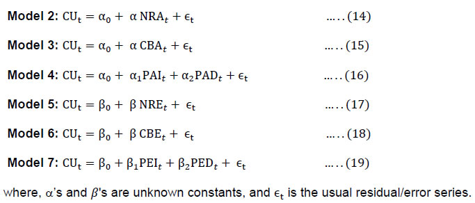 Models 2-3 and Models 5-6 explain CU with the help of popular summary measure ‘Net Response’ (i.e., ‘Balance Statistics’) or CB Index based on responses on either assessment for the survey quarter or the one-quarter-ahead expectation. It is likely that a rise (fall) in NRA/NRE or CBA/CBE would result in a rise (fall) in CU, so the coefficient α and β are expected to be positive. Model 4 (Eqn. 16), however, regress CU on percentage responses on assessment, separately for ‘rise’ (PAI) and ‘fall’ (PAD). If NR contains all information of the survey responses, then the coefficients of PAI and PAD would be same in magnitude but opposite in sign. In other words, the NR-based regression imposes the symmetry of coefficients of proportion of ‘increase/rise’ and ‘decrease/fall’ responses. In practice, however, this assumption or restriction of symmetry may not hold good. For example, Cunningham (1997) rejects the symmetry for majority of the questions/variables tested. Further, a common perception would suggest PAI having a positive impact on CU, and PAD an adverse/opposite effect. Model 7 (Eqn. 19) explains CU with the help of qualitative responses on one-quarter ahead expectation, and signs of the model parameters are expected to be in line with those in Model 4. Table 6 displays the parameter estimated for Models 2-4. Similar estimates for Models 5-7 are given in Table 7. Empirical estimates in Table 6, show that the impact of NRA on CU, as expected, is positive and statistically significant at 1 per cent level. The adjusted-R2 (at 0.44) for Model 2 is reasonably high. The impact of CBA (Model 3) also appears positive and significant, though the overall performance of this model is relatively worse (adjusted-R2 being at 0.38). By the same measure of goodness of fit, Model 4, which explains CU by using responses on alternative options in qualitative questions (instead of summary statistics like Net Response) with adjusted-R2 value of 0.65 is much superior to Models 2-3. This finding implies that we lose information for CU by summarising the qualitative responses in the form of Net Response. One apparent inconsistency in the estimated model perhaps is the positive sign of the coefficient of the PAD in Model 4. However, we show in the following section show that (a) this apparent anomaly in the sign of PAD is due to the multi-collinearity between PAI and PAD, and (b) adjusting for multi-collinearity reveals that the overall impact of PAI and PAD on CU are consistent with common perception (i.e., the effect of PAI on CU is positive and that of PAD is negative). The results for qualitative responses on expectation (Table 7) are also similar to the case of responses on assessment (Table 6), though the strength of the relationship between CU and qualitative responses became relatively weaker. Two interesting findings can be made from Tables 6-7. First, the goodness of fit improves if the model uses responses on ‘rise' and ‘fall' separately instead of using summary measures like NR or CB index. Second, assessment for a quarter is a better predictor of CU for the same quarter than the expectation formed one quarter before. | Table 6: Estimated Models for CU - Using responses on assessment for the same quarter | | Model | Constant | NRAt | CBAt | PAIt | PADt | R2 | R2adj. | | Model 2 | 72.6591
(0.00000) | 0.2468
(0.00000) | | | | 0.46 | 0.44 | | Model 3 | 65.9902
(0.00000) | | 0.1699
(0.00222) | | | 0.41 | 0.38 | | Model 4 | 54.0673
(0.00000) | | | 0.6680
(0.00000) | 0.2259
(0.00380) | 0.67 | 0.65 | Note: The figures in parentheses denote the p-values corresponding to tests of significance of respective parameters. All parameters are statistically significant at 1per cent level.
Source: Authors’ estimates. |
| Table 7: Estimated Models for CU - Using responses on expectation one quarter ahead | | Model | Constant | NREt | CBEt | PEIt | PEDt | R2 | R2adj. | | Model 5 | 69.4039
(0.00000) | 0.2873
(0.00002) | | | | 0.33 | 0.31 | | Model 6 | 66.0073
(0.00000) | | 0.1436
(0.00104) | | | 0.16 | 0.12 | | Model 7 | 48.6677
(0.00000) | | | 0.7514
(0.00000) | 0.3673
(0.04120) | 0.53 | 0.51 | Note: The figures in parentheses denote the p-values corresponding to tests of significance of respective parameters. It may be noted that all parameters are statistically significant at 1per cent level of significance.
Source: Authors’ estimates. | IV.2.1.1 Sign of Coefficients in Estimated Models The positive signs of parameter estimate corresponding to PADt and PEDt in Models 4 & 7 appear inconsistent with general perception. We attribute this phenomenon to the high degree of negative correlation between PAIt and PADt, (at -0.7531) and between PEIt and PEDt (at -0.6990). These correlations are expected for the identities in the Eqns. (3)-(4). For example, given the identity in Eqn. (3), i.e., PAIt + PADt + PANt = 100 for all t, and given PANt, a rise (fall) in PADt would result in a fall (rise) in PAIt and vice-versa. The simultaneity in changes in PAIt and PADt in the opposite direction would result in negative correlation coefficient between the two variables. A similar argument using the identity in Eqn.(4) would imply negative correlation coefficient between PEIt and PEDt. The identified near multicollinearity in Model 4 (Eqn.16) and Model 7 (Eqn. 19) may result in incorrect signs or insignificance of some coefficients, but model performance in predicting the dependent variable will not suffer much, instead may improve sometimes (Ramathan, 2002, pp. 211-14; Gujarati and Sangeetha, 2007, pp. 358-66). We postulate the relationships between PAIt and PADt, and between PEIt and PEDt as: 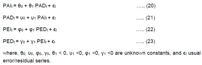 From Eqn. (16), one unit rise in PADt would have a direct impact on CU by the α2 unit. Simultaneously, by Eqn. (20), PAIt will rise by θ1, which will lead to an indirect impact on CU by (α1 θ1) units. The sum of the direct and the indirect effects of one unit rise in PAD on CU is (α2 + α1 θ1). The common perception expects (α2 + α1 θ1) to have a negative sign. In Table 8 we present the total impact of one unit change in PAD or PAI on CU (Eqn. 16) and the same of one unit change in PED or PEI (Eqn. 19). The empirical estimates of models given in Eqns. (20)-(23) are presented in Table 9. As expected, estimates of θ1, υ1, φ1, and γ1 are not only having negative signs but statistically significant at 1 per cent level. Finally, we estimate the total impact of one unit change in PAD or PED on CU following the formula given in the last column of the Table 8. Table 10 reports the quantified impacts so obtained. As seen earlier (Tables 6-7), a rise (fall) in PAI or PEI results in the rise (fall) in CU. However, unlike the earlier results, Table 10 shows that a change in PAD or PED affects CU negatively. | Table 8: Impact of Changes in Qualitative Responses on CUt | | Scenario* | Direct Impact on CUt | Indirect Impact on CUt | Combined/ Total Impact on CUt | Sign of Total Impact | Case 1:
PAIt increases by one unit. | Eqn.(16) says CUt changes by α1 units. | Eqn.(21) & Eqn.(16) imply PADt changes by υ1 units, resulting in a change of CUt by α2 x υ1 units. | CUt changes by (α1 + α2 x * υ1) units. | (α1 + α2 x υ1) > 0 | Case 2:
PADt increases by one unit. | Eqn.(16) says CUt changes by α2 units. | Eqn.(20) & Eqn.(16) imply PAIt changes by θ1 units, resulting in a reduction of CUt by α1 x θ1 units. | CUt changes by (α2 + α1 x θ1) units. | (α2 +α1 x θ1) < 0 | Case 3:
PEIt increases by one unit. | Eqn.(19) says CUt changes by β1 units. | Eqn.(23) & Eqn.(19) imply PEDt changes by γ1 units, resulting in a reduction of CUt by β2 x γ1 units. | CUt changes by (β1 + β2 x γ1) units. | (β1 + β2 x γ1) > 0 | Case 4:
PEDt increases by one unit. | Eqn.(19) says CUt changes by β2 units. | Eqn.(22) & Eqn.(19) imply PEIt changes by φ1 units, resulting in a reduction of CUt by β1 x φ1. | CUt changes by (β2 + β1 x φ1) units. | (β2 + β1 x φ1) < 0 | Note: ‘*’ We consider only the scenarios of increase in percentage response by 1 unit. In case of decrease by one unit, the impact would be of the same magnitude but with reverse sign/direction.
Source: Authors’ estimates. |
| Table 9: Estimated Relationship between PAI & PAD and between PEI & PED | | Model/Equation | Constant | PAIt | PADt | PEIt | PEDt | R2 | R2adj. | Eqn.(20):
PAIt = θ0 + θ1PADt + ϵt | 39.3721
(0.00000) | | - 0.8333
(0.00000) | | | 0.57 | 0.56 | Eqn.(21):
PADt = υ0 + υ1 PAIt + ϵt | 33.9346
(0.00000) | - 0.6806
(0.00000) | | | | 0.57 | 0.56 | Eqn.(22):
PEIt = φ0 + φ1 PEDt + ϵt | 39.6635
(0.00000) | | | | - 0.9362
(0.00000) | 0.49 | 0.47 | Eqn.(23):
PEDt = γ0 + γ1 PEIt + ϵt | 26.1096
(0.00000) | | | - 0.5219
(0.00000) | | 0.49 | 0.47 | Note: The figures in parentheses denote the p-values corresponding to tests of significance of respective parameters. It may be noted that all parameters are coming to be statistically significant at 1per cent level of significance.
Source: Authors’ estimates. |
| Table 10: Quantified Impact of Changes in Qualitative Responses on CUt | | Scenario | Direct Impact on CUt | Indirect Impact on CUt | Combined/ Total Impact on CUt | Remarks (on Sign of Total Impact) | | Case 1: | Eqn.(16) implies | Eqn.(21) & Eqn.(16) imply | (α1 + α2 x υ1) = 0.5143 | Correct Sign | | PAIt increases by one unit. | α1 = 0.6680 | α2 x υ1
= 0.2259 x - 0.6806
= -0.1537 | | Case 2: | Eqn.(16) implies | Eqn.(20) & Eqn.(16) imply | (α2 + α1 x θ1) = - 0.3307 | Correct Sign | | PADt increases by one unit. | α2 = 0.2259 | α1 x θ1
= 0.6680 x - 0.8333
= - 0.5566 | | Case 3: | Eqn.(19) implies | Eqn.(23) & Eqn.(19) imply | (β1 + β2 x γ1) = 0.5597 | Correct Sign | | PEIt increases by one unit. | β1 = 0.7514 | β2 x γ1
= 0.3673 x - 0.5219
= - 0.1917 | | Case 4: | Eqn.(19) implies | Eqn.(22) & Eqn.(19) imply | (β2 + β1 x φ1) = - 0.3362 | Correct Sign | | PEDt increases by one unit. | β2 = 0.3673 | β1 x φ1= 0.7514 x - 0.9362= - 0.7035 | | Source: Authors’ estimates. | Having confirmation that impact of change in PAI/PEI or PAD/PED on CU are indeed in expected line (though the strong multi-collinearity between PAI and PAD, and between PEI and PED resulted into incorrect signs of the coefficients of PAD and PED in Eqn. 3 & 6, respectively), we plot out-of-sample forecasts of CU using Models 1-4, along with realised estimates of CU in Chart 1. It is clearly seen that the Models 2-3 which use summary measures of qualitative responses on assessment, i.e., NRA or CBA, have a tendency to overestimate CU. However, the most closed forecasts among these models are obtained from Model 4 that considers both PAI and PAD as two regressors (instead of summarising them, say as NRA). The out-of-sample forecast performance of the models using responses on expectations, i.e., Models 5-7, also share a broad pattern similar to those of their counterpart models using responses on the assessment (Chart 2).
IV.2.2 Linear Models: Further Empirical Results The simple linear models estimated earlier were useful to confirm that the impact of one unit change in PAI/PEI or PAD/PED on CU is in correct direction even though the strong multicollinearity among the regressors may result into incorrect sign for some coefficients. In this section, we examine the linear relationship further by factoring into the possible impact of lagged-CU. Accordingly, models in Models 2-7 given in Eqn. (14)-(19) are modified as below; 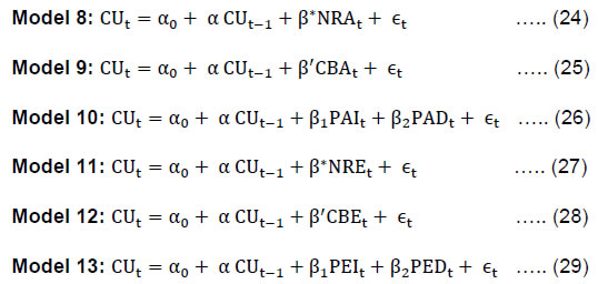 The Models 8-10 relate to qualitative assessment of current quarters. Estimates of these models (Table 11) show that lagged-CU turns out to be statistically insignificant (at 1 per cent level) in presence of either summary measure, such as NRA and CBA, or when both responses of increase and decrease enter separately as regressors. Interestingly, judging by R2adj., model using increase and decrease responses separately as regressors (Model 10) fits much better than the use of any summary measure (Models 8-9). The empirical estimates of Models 11-13, which are developed based on one-quarter ahead outlook or expectations, also reveal a similar broad picture (Table 12). Though lagged-CU has either gained significance or improved slightly, the goodness of fit of any of these models is relatively weaker when compared with its counterpart using qualitative responses on assessment. | Table 11: Estimated Models for CU - Using responses on Assessment for the same quarter | | Model | Constant | CUt-1 | NRAt | CBAt | PAIt | PADt | R2 | R2adj. | | Model 8 | 58.0857
(0.00000) | 0.1988
(0.15810) | 0.2111
(0.00017) | | | | 0.50 | 0.47 | | Model 9 | 46.3416
(0.00000) | 0.2319
(0.09790) | | 0.1838
(0.00029) | | | 0.49 | 0.46 | | Model 10 | 59.4401
(0.00000) | -0.0868
(0.47010) | | | 0.7239
(0.00000) | 0.2171
(0.02120) | 0.71 | 0.69 | Note: The figures in parentheses denote the p-values corresponding to tests of significance of respective parameters.
Source: Authors’ estimates. |
| Table 12: Estimated Models for CU - Using responses on expectation one quarter ahead | | Model | Constant | CUt-1 | NREt | CBEt | PEIt | PEDt | R2 | R2adj. | | Model 11 | 46.7102
(0.00002) | 0.3189
(0.00002) | 0.2268
(0.00253) | | | | 0.43 | 0.40 | | Model 12 | 33.4213
(0.00136) | 0.3980
(0.00628) | | 0.1587
(0.01830) | | | 0.37 | 0.34 | | Model 13 | 42.5754
(0.00003) | 0.1447
(0.29100) | | | 0.6366
(0.00008) | 0.2538
(0.13000) | 0.55 | 0.51 | Note: The figures in parentheses denote the p-values corresponding to tests of significance of respective parameters.
Source: Authors’ estimates. | We depict out-of-sample forecasts of Models 8-10 along with Model 1 in Chart 3. The forecasts, here again, exhibit the pattern observed earlier (in Chart 1) – the models using summary of assessment, such as NRA or CBA (Models 8-9) usually generate forecasts with an upward bias. However, when assessment with an ‘increase’ and that with a ‘decrease’ response are used as two separate regressors (instead of summarising them, say through NRA) as done in Model 10, forecasts become much closer to the realised CU values. Interestingly, a similar pattern is also observed for corresponding models with responses on expected CU, i.e., Models 11-13 (Chart 4).
IV.2.3 Non-Linear Models: Regime Switching Regressions We explore non-linearity through regime-switching regression, and estimate Models 14-16, relating CU with NRA or CBA or with both PAI and PAD (Table 13). We estimate another three models, viz., Models 17-19, for responses on expectations, viz., NRE, CBE and separate use of both PEI and PED as regressors (Table 14). As expected, the performance of forecasts of these non-linear models (Models 14-19) appears to have improved when compared with any of the corresponding linear models (Chart 5-6).
| Table 13: Estimated Models for CU - Using responses on assessment for the same quarter | | Model | Constant | NRAt | CBAt | PAIt | PADt | | State | State | State | State | State | | 1 | 2 | 1 | 2 | 1 | 2 | 1 | 2 | 1 | 2 | | Model 14 | 32.889 | 62.116 | 0.390 | 0.140 | | | | | | | | Model 15 | 58.913 | 67.062 | | | 0.254 | 0.175 | | | | | | Model 16 | 73.144 | 52.383 | | | | | 0.251 | 0.759 | -0.357 | 0.227 | | Source: Authors’ estimates. |
| Table 14: Estimated Models for CU - Using responses on expectations one quarter ahead | | Model | Constant | NREt | CBEt | PEIt | PEDt | | State | State | State | State | State | | 1 | 2 | 1 | 2 | 1 | 1 | 2 | 1 | 2 | 1 | | Model 17 | 75.407 | 24.793 | 0.007 | 0.425 | | | | | | | | Model 18 | 70.090 | 72.471 | | | 0.064 | 0.081 | | | | | | Model 19 | 88.430 | 75.662 | | | | | 0.015 | 0.274 | -1.287 | -0.821 | | Source: Authors’ estimates. |
IV.3 Evaluation of Models: Out-of-Sample Forecast Errors The Models 1-19 are estimated recursively starting with CU data for first 20 quarters, i.e., spanning from Q1:2008-09 to Q4:2012-13 and forecast is generated for Q1:2013-14 and Q2:2013-14 using assessment for Q1:2013-14 and expectation for Q2:2013-14, respectively, from IOS. At every successive iteration, an additional data point at the end of the data period is incorporated and forecasts are generated for the next two time points. For a formal evaluation of competing models, four alternative measures of out-of-sample forecast errors are given in Eqns. (9)-(12), viz., Mean Absolute Error (MAE), Root-Mean-Square-Error (RMSE), Mean Absolute Percentage Error (MAPE), and Root-Mean-Square-Percentage-Error (RMSPE) are computed. Table 15 presents estimates of these performance measures with respect to all competing models in a few panels, viz., Panels A-D. While the Panel A shows errors of Model 1, which model CU based on only its own lagged-value, each of the remaining panels covers results for three models each for assessment and expectations. Table 15 clearly reveals a few interesting observations. First, the summarized qualitative responses, viz., CB index, sometimes performs worse than lagged-CU values (Model 1) in tracking or predicting CU. For example, the values of error measures MAE, RMSE, MAPE and RMSPE are 1.97, 2.48, 2.74 and 3.48, respectively for Model 1, but are higher at 2.22, 2.63, 3.08 and 3.67, respectively for Model 6 (which used CBE to predict one-quarter-ahead CU). Second, a strategy of considering responses on ‘rise' and ‘fall' separately in the model is much superior to the use of lagged-CU values or summary measures like Net Responses or CB index. This is so because among the three models for assessment presented under each of Panels B-D, the one using ‘increase/rise’ and ‘decrease/fall’ responses separately yields the least errors. Third, as expected, out-of-sample forecast errors of the models based on responses on ‘assessment for current quarters’ are relatively lower than corresponding model using ‘one-quarter-ahead expectations'. Fourth, a model based on both qualitative responses and lagged-CU values performs better than corresponding model that uses only lagged-CU value or qualitative responses. Finally, non-linear models improve tracking or forecasting accuracy over their linear counterparts. | Table 15: Out-of-Sample Forecast Errors: Four Alternative Measures | | Model / Equation | Magnitude of Error | Magnitude of Percentage Error | | MAE | RMSE | MAPE | RMPSE | | (A). AR Model | | | | | | Model 1: CUt = α0 + α CUt-1 + ϵt | 1.97 | 2.48 | 2.74 | 3.48 | | (B). Simple Linear Models | | | | | | Assessment | | | | | | Model 2: CUt = α0 + α NRAt + ϵt | 1.75 | 2.02 | 2.41 | 2.81 | | Model 3: CUt = α0 + α CBAt + ϵt | 1.85 | 2.12 | 2.55 | 2.93 | | Model 4: CUt = α0 + α1PAIt + α2PADt + ϵt | 1.06 | 1.23 | 1.45 | 1.69 | | Expectation/Outlook | | | | | | Model 5: CUt = β0 + β NREt + ϵt | 1.87 | 2.26 | 2.59 | 3.16 | | Model 6: CUt = β0 + β CBEt + ϵt | 2.22 | 2.63 | 3.08 | 3.67 | | Model 7: CUt = β0 + β1PEIt + β2 PEDt + ϵt | 1.40 | 1.61 | 1.92 | 2.19 | | (C). Linear Models with Lagged-CU | | | | | | Assessment | | | | | | Model 8: CUt = α0 + α CUt-1 + β*NRAt + ϵt | 1.74 | 1.98 | 2.40 | 2.78 | | Model 9: CUt = α0 + α CUt-1 + β′CBAt + ϵt | 1.82 | 2.11 | 2.52 | 2.92 | | Model 10: CUt = α0 + α CUt-1 + β1PAIt + β2PADt + ϵt | 1.07 | 1.21 | 1.38 | 1.66 | | Expectation/Outlook | | | | | | Model 11: CUt = α0 + α CUt-1 + β*NREt + ϵt | 1.80 | 2.09 | 2.36 | 2.93 | | Model 12: CUt = α0 + α CUt-1 + β′CBEt + ϵt | 1.86 | 2.32 | 2.58 | 3.25 | | Model 13: CUt = α0 + α CUt-1 + β1PEIt + β2PEDt + ϵt | 1.39 | 1.59 | 1.90 | 2.18 | | (D). Regime-Switching Models | | | | | | Assessment | | | | | | Model 14: CUt = α0s + βs*NRAt + ϵt, s ∈ S = {1,2} | 1.25 | 1.59 | 1.70 | 2.18 | | Model 15: CUt = α0s + β′sCBAt + ϵt, s ∈ S = {1,2} | 1.68 | 2.05 | 2.29 | 2.80 | | Model 16: CUt = α0s + β1sPAIt + β2sPADt + ϵt, s ∈ S{1,2} | 0.48 | 0.62 | 0.66 | 0.86 | | Expectation/Outlook | | | | | | Model 17: CUt = α0s + βs*NREt + ϵt, s ∈ S = {1,2} | 1.41 | 2.08 | 1.95 | 2.92 | | Model 18: CUt = α0s + β′sCBEt + ϵt, s ∈ S = {1,2} | 1.47 | 2.11 | 2.01 | 3.20 | | Model 19: CUt = α0s + β1sPEIt + β2sPEDt + ϵt, s ∈ S = {1,2} | 0.93 | 1.29 | 1.27 | 1.77 | | Source: Authors’ estimates. | V. Conclusion The Net Response (NR), also known as Balance Statistics (BS), has been a widely used measure of summarising qualitative survey responses. It is defined as the difference between the percentage of responses for a ‘rise/improvement' and that indicating a ‘fall/deterioration' for an underlying economic parameter or reference variable. In India, conducting such qualitative surveys is of much recent origin, and studies on assessing the usefulness of the qualitative results obtained from those surveys in tracking or forecasting corresponding reference variables are scanty. In this paper, an attempt is made to see how good are the qualitative indicators of capacity utilisation for the manufacturing sector which are disseminated by the Reserve Bank of India (RBI) based on its Industrial Outlook Survey (IOS) conducted at a quarterly frequency. For comparable corresponding reference, we consider the quantitative estimate of CU compiled by the RBI based on data on actual production and installed capacity of a sample of manufacturing companies which are collected through another quarterly survey, viz., the Order Book, Inventory and Capacity Utilisation Survey (OBICUS). Empirical results reveal a few interesting findings. First, the summarisation of qualitative responses through well-known popular measures or diffusion indices like the net response (NR) leads to the loss of much information about the target variable, and at times may not be very useful in tracking or predicting the corresponding quantitative variable. In particular, the performance of NR on both ‘assessment of CU during the survey quarter' and ‘expectation formed one-quarter before' appears to have poor tracking or predictive ability. Second, a much better strategy is to use the percentage responses for ‘rise/ improvement in CU’ and ‘fall/deterioration’ separately in any modeling exercise. Third, as expected, responses on ‘assessment in the survey quarter’ are more informative than ‘expectation formed in the previous quarter’. The empirical results presented in the paper have significant policy implications, particularly for quantifying market expectations and making a forward-looking assessment of the economy. Analysts engaged in short-run predictions for the manufacturing sector may find these results useful for extracting more meaningful information from survey results. Future research may focus on qualitative indicators on other economic variables covered in various surveys and on experimenting with other quantifying techniques.
References Anderson, Oskar, Jr. (1952). The Business Test of the IFO-Institute for Economic Research, Munich, and Its Theoretical Model. Revue de l’Institut International de Statistique/Review of the International Statisticsl Institute, 20(1): 1-17. Artis, M. J., Marcellino, M. & Proietti, T. (2004). Dating Business Cycles: A Methodological Contribution with an Application to the Euro Area. Oxford Bulletin of Economics and Statistics, 66, 537– 565. Balcombe, Kelvin (1996). The Carlson-Parkin Method Applied to NZ Price Expectations using QSBO Survey Data. Economics Letters, 51:51-57. Bardaji, J., Clavel, L. & Tallet, F. (2009). Constructing a Markov-switching Turning Point Index Using Mixed Frequencies with an Application to French Business Survey Data. Journal of Business Cycle Measurement and Analysis, vol. 2009/2, 111-132. Bauer, Paul W. (1990). A Re-examination of the Relationship between Capacity Utilization and Inflation. Review, Federal Reserve Bank of Cleveland, Q3. Baum, L.E., Petrie, T., Soules, G. & Weiss, N. (1970). A Maximization Techinque occurring in the Statistical Analysis of Probabilistic Functions of Markov Chains. Annals of Mathematical Statistics, 41,164–171. Bellone, B. & Saint-Martin, D. (2003). Detecting Turning Points with Many Predictors through Hidden Markov Models. French Forecasting and Economic Analysis Directorate. Bernardelli, M. (2015). The procedure of business cycle turning points identification based on hidden Markov models. Prace i Materiały Instytutu Rozwoju Gospodarczego IRG, 96, 5-23. Berndt, Ernst R. & Catherine J. Morrison (1981). Capacity Utilization Measures: Underlying Economic Theory and an Alternative Approach. The American Economic Review, Vol. 71, No. 2, Papers and Proceedings of the Ninety-Third Annual Meeting of the American Economic Association, May: 48-52. Carlson, John A. (1975). Are Price Expectations Normally Distributed? Journal of the American Statistical Association, Vol. 70, No. 352, December: 749-54. Carlson, John A. & Michael Parkin (1975). Inflation Expectations. Economica, New Series, Vol. 42, No. 166, May: 123-38. Camacho, M., & Perez Quiros, G., and Poncela, P. (2012). Extracting nonlinear signals from several economic indicators. Journal of Applied Econometrics, 30: 1073- 1089. Cunningham, Alastair (1997). Quantifying Survey Data. Quarterly Bulletin, Bank of England, August: 292-300. Das, Abhiman, Kajal Lahiri & Yongchen Zhao (2019). Inflation Expectations in India: Learning from Household Tendency Surveys. International Journal of Forecasting, 35: 980-993. Das, Marcel & Arthur van Soest (1997). Expected and Realised Income Changes: Evidence from the Dutch Socio-Economic Panel. Journal of Economic Behaviour and Organization, 32: 137-54. Davies, Anthony & Kajal Lahiri (1995). A New Framework for Analyzing Survey Forecasts using Three-Dimensional Panel Data. Journal of Econometrics, 68: 205-27. D’Elia, Enrico (2005). Using the Results of Qualitative Surveys in Quantitative Analysis. Working Paper No. 56, Istituto Di Studi E Analisi Economica, September. Diebold, F. X. & G. D. Rudebusch (1996). Measuring business cycles: a modern perspective. The Review of Economics and Statistics, 78, 67–77. Diebold, F.X., J.-H. Lee, & G.C. Weinbach. (1994). Regime switching with time-varying transition probabilities in Nonstationary Time Series Analysis and Cointegration, C.P. Hargreaves, ed. Oxford and New York. Oxford University Press, 283-302. Divatia, V.V. & Ravi Verma (1970). Index of Potential Utilisation Ratio for Manufacturing Industries in India. RBI Bulletin, April: 574-601. Dominitz, Jeff & Charles F. Manski (2003). How Should We Measure Consumer Confidence (Sentiment)? Evidence from the Michigan Survey of Consumers. Working Paper 9926, NBER Working Paper Series, August, National Bureau of Economic Research. Dotsey, Michael & Thomas Stark (2005). The Relationship Between Capacity Utilisation and Inflation. Business Review, Q2, Federal Reserve Bank of Philadelphia. Driver, Ciaran & Giovanni Urga (2004). Transforming Qualitative Survey Data: Performance Comparisons for the UK. Oxford Bulletin of Economics & Statistics, 66 (1-iv): 71-89. Filardo, Andrew & Gordon Stephen (1998). Business Cycle Durations. Journal of Econometrics, 85(1): 99-123. Galstyan, Martin & Vahe Movsisyan (2010). Quantification of Qualitative Data: the Case of the Central Bank of Armenia. IFC Bulletin, 33: 202-15. Garner, C. Allan (1994). Capacity Utilization and US Inflation. Economic Review, Federal Reserve Bank of Kansas City, Fourth Quarter. Gittings, Thomas A. (1989). Capacity Utilization and Inflation. Economic Perspective, Federal Reserve Bank of Chicago. Goldfeld, S.M. & R.E. Quandt. (1973). A Markov model for switching regressions. Journal of Econometrics, 1(1):3-15. Gujarati, Damodar N. & Sangeetha (2007), Basic Econometrics, Fourth Edition, Special Indian Edition, Tata McGraw-Hill Publishing Company Ltd. Hamilton, J.D. (1989). A new approach to the economic analysis of non-stationary time series and the business cycle. Econometrica, 57, 357-384. Hamilton, J. D. & R. Susmel (1994). Autoregressive conditional heteroskedasticity and change in regime. Journal of Econometrics, 64, 307–333. Henzel, Steffen & Timo Wollmershäuser (2005). An Alternative to the Carlson-Parkin Method for the Quantification of Qualitative Inflation Expectations: Evidence from the Ifo World Economic Survey. Ifo Working Paper No. 9, June, Ifo Institute for Economic Research at the University of Munich. Kim, CJ. & Murray, CJ.(2002). Permanent and Transitory Components of Recession. Empirical Economics, 27,163-183. Klein, L.R. (1960). Some Theoretical Issues in the Measurement of Capacity. Econometrica, 28: 272-86. Klein, Lawrence R. & Robert Summers (1966). The Wharton Index of Capacity Utilization, University of Pennsylvania, Wharton School of Finance and Commerce, Economics Research Unit. Klein, L.R. & R.S.Preston (1967). Some New Results in the Measurement of Capacity Utilisation. The American Economic Review, 57: 34-58. Knöbl, Adalbert (1974). Price Expectations and Actual Price Behaviour in Germany. International Monetary Staff Papers, 21: 83-100. Kock, Gabriel S.P. de & Tania Nadal-Vicens (1996). Capacity Utilization-Inflation Linkages: A Cross-Country Analysis. Research Paper No. 9607, Federal Reserve Bank of New York, April. Löffler, Gunter (1999). Refining the Carlson-Parkin Method. Economics Letters, 64: 167-71. Mitchell, James (2002). The Use of Non-Normal Distributions in Quantifying Qualitative Survey Data on Expectations. Economics Letters, 76: 101-07. Mitchell, James, Richard J. Smith & Martin R. Weale (2013). Efficient Aggregation of Panel Qualitative Survey Data. Journal of Applied Econometrics, 28: 580-603. Musigchai, Chatwaruth (2008). Relationship with survey data providers: the Bank of Thailand’s experiences. IFC Bulletin, No 28, August, Bank for International Settlements. Müller, Christian (2010). You CAN Carlson-Parkin. Economic Letters, 108: 33-35. Nakibullah, Ashraf & Bassim Shebeb (2013). The Relationship Between Capacity Utilization and Inflation: The Case of Bahrain. The Global Journal of Finance and Economics, 10(2): 139-149. Nilsson, Ronny (2001). Business Tendency Surveys in OECD Countries – Methodological Review, OECD. OECD (2003). Business Tendency Surveys – A Handbook, Organisation for Economic Co-Operation and Development (OECD). Omana, Lekshmi & Om Prakash Mall (2015). Forward Looking Surveys for Tracking Indian Economy: An Evaluation. IFC Bulletin, No. 39, Bank for International Settlements, April: 1-14. Paul, Samuel (1974). Growth and Utilisation of Industrial Capacity. Economic and Political Weekly, 9(49): 2025-2032. Pesaran, M. H. (1985). Formation of Inflation Expectations in British Manufacturing Industries. The Economic Journal, 95(380): 948-75. Pesaran, M. H. (1987). The Limits to Rational Expectations, Basil Blackwell, Oxford. Ragan, James F. (1976). Measuring Capacity Utilization in Manufacturing. Quarterly Review, Federal Reserve Bank of New York, Winter: 13-20. Ramathan, Ramu (2002). Introductory Econometrics with Applications, Fifth Edition, Thomson, South-Western. RBI (2009). Quarterly Industrial Outlook Survey: Trends since 2000-01. RBI Bulletin, Reserve Bank of India, October: 1947-86. RBI (2011). Quarterly Order Books, Inventories and Capacity Utilisation Survey: April-June 2011 (Round 14). RBI Bulletin, December. RBI (2015). Position of Order Books, Inventories and Capacity Utilisation for the Quarters October 2013 to March 2015. RBI Bulletin, September: 55-60. RBI (2016a). Position of Order Books, Inventories and Capacity Utilisation for the Quarters April 2015 to March 2016. RBI Bulletin, Reserve Bank of India, September: 29-32. RBI (2016b). Minutes of the Monetary Policy Committee Meeting, October 3-4, 2016 [Under Section 45ZL of the RBI Act, 1934]. Press Release, Reserve Bank of India, October 18, 2016. RBI (2017a). The Industrial Outlook Survey, 2016-17. RBI Bulletin, Reserve Bank of India, June: 25-40. RBI (2017b). Minutes of the Monetary Policy Committee Meeting, April 5-6, 2017 [Under Section 45ZL of the RBI Act, 1934]. Press Release, Reserve Bank of India, April 20, 2017. RBI (2017c). Quarterly Order Books, Inventories and Capacity Utilisation Survey (OBICUS) –Round 38 (Q1:2017-1). Press Release, Reserve Bank of India, October 4, 2017. RBI (2018). Minutes of the Monetary Policy Committee Meeting, April 4-5, 2018 [Under Section 45ZL of the RBI Act, 1934]. Press Release, Reserve Bank of India, April 19, 2018. RBI (2019). Minutes of the Monetary Policy Committee Meeting, April 2-4, 2019 [Under Section 45ZL of the RBI Act, 1934]. Press Release, Reserve Bank of India, April 18, 2019. RBI (2020). Minutes of the Monetary Policy Committee Meeting, February 4-6, 2020 [Under Section 45ZL of the RBI Act, 1934]. Press Release, Reserve Bank of India, February 20, 2020. Reserve Bank of India (RBI), RBI Bulletin: Various Press/Web/Data Releases, and Policy statements on website (www.rbi.org.in). Rosenblatt-Wisch, Rina & Rolf Scheufele (2014). Quantification and Characteristics of Household Inflation Expectations in Switzerland. SNB Working Papers, Swiss National Bank, 11/2014. Samanta, G.P. & Sayantika Bhowmick (2018). Are Survey-based Indicators on Capacity Utilisation Rates Informative? – An Empirical Analysis for Select RBI Surveys. CIRET Conference, September 11-15, 2018, Rio de Janeiro, Brazil. Seitz, Helmut (1988). The Estimation of Inflation Forecasts from Business Survey Data. Applied Economics, 20: 427-38. Smith, J. & Mcaleer, M. (1995). Alternative Procedures for Converting Qualitative Response Data to Quantitative Expectations: An Application to Australian Manufacturing. Journal of Applied Econometrics, 10(2): 165-85. Theil, H. (1952). On the Time Shape of Economic Microvariables and the Munich Business Test. Revue l’Institut International de Statistique / Review of the International Statisticsl Institute, 20: 105-20. Viterbi, A. J. (1967). Error Bounds for Convolutional Codes an and Asymptotically Optimum Decoding Algorithm. IEEE Transactions on Information Theory, IT-13: 260 - 269. Weale, Martin (2014). Spare Capacity and Inflation. Speech given at the Confederation of British Industry, Belfast, June 18, Bank of England. Wooldridge, Jeffrey M. (2000). Introductory Econometrics – A Modern Approach, Fourth Edition, Cengage Learning. Yoo, Peter S. (1995). Capacity Utilisation and Prices within Industries. Review, Federal Reserve Bank of St. Louis, September/October.
Annex 1: Regime-Switching Regression Elements of the Viterbi path are calculated using the Viterbi algorithm (Viterbi 1967) and the parameters of the HMM are estimated by iteratively maximizing the expected log-likelihood of the observations derived on the basis of the Baum-Welch algorithm (Baum et al., 1970). For sake of simplicity, a two-state HMM was considered in this paper, by fragmenting the time series into two types of periods: those associated with relatively good conditions and those connected with worse situation. The state space may be extended to higher level scales leading to enriching the analysis, subject to interpretation (Artis et al., 2004; Kim and Murray, 2002). |