“… AND WHEREAS the primary objective of the monetary policy is to maintain price stability while keeping in mind the objective of growth; AND WHEREAS the monetary policy framework in India shall be operated by the Reserve Bank of India.” [Excerpted from Preamble to the Reserve Bank of India (RBI) Act, 1934
(amended by the Finance Act, 2016)] 1. Introduction I.1 Central banks stand for stability – price stability; exchange rate stability; financial stability; regime stability. These nuances of stability fill the lexicon of their vision and mission statements. So sworn are they to the preservation of stability that their day-to-day functioning becomes enigmatic. Illustratively, central banks are destined to live with shocks on a daily basis, but avoid giving ‘unpleasant monetary surprises’ in the conduct of monetary policy, conscientiously impelled to engage in interest rate smoothing or ‘baby-stepping’ in their policy actions and stances (Chart I.1). 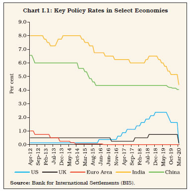 I.2 Above all, it is regime shifts that draw forth their stiffest resistance. After all, monetary policy frameworks crystallise after protracted and often painful confrontations with the challenges of aligning goals and instruments in the face of long and variable lags, avoiding time inconsistency, remaining forward-looking and accountable, and importantly, free of fiscal dominance. Consequently, it is only a tectonic change – in their environment without, or in their philosophy within – which can force them to make a step in the dark to a new regime. Typically, they are prompted to make the leap by the fear of losing control over instruments or operating procedures. The tryst with and abandonment of policy regimes with monetary aggregates as operating and/or intermediate targets in the 1980s and 1990s, for example, was candidly described by John Crow, former Governor of the Bank of Canada: “We did not leave the monetary aggregates; they left us.” The adoption of inflation targeting in the early 1990s, too, was a vault into the unknown. The critics’ view was that, like the aurora australis, it was an exotica that can happen only UNDER (New Zealand) down under (Australia). At the time of releasing this Report, 401 countries and countinghave adopted it2. At this juncture, however, inflation targeting frameworks around the world are being reviewed and time will tell whither goes FIT in the future (Box I.1). Box I.1
Insights from Country Framework Reviews Inflation targeting (IT) as a monetary policy framework continues to evolve, based on individual country experiences. Although formal frameworks differ widely across countries, there have been notable operational similarities in target setting; policy communication; and performance assessment. At the same time, there is also more variability than in the early years of its adoption, especially in how the IT frameworks are reviewed and how financial stability considerations are accounted for in the setting of monetary policy (Wadsworth, 2017). Framework reviews provide both a ‘laboratory’ setting and a rich diversity of experiences thrown up by interactions with country-specific characteristics to introspect and to learn. Interestingly, several such reviews are coinciding, offering glimpses into and around the future of IT. IT was formally adopted by New Zealand with the passing of the Reserve Bank of New Zealand Act of 1989 by the Parliament on December 15, 1989 and took effect in February 1990. For the first time, price stability was defined as an inflation rate between 0 and 2 per cent to be achieved by December 1992. The Governor was invested with sole legal responsibility for achieving and maintaining inflation within the defined target. Several iterations later and following a framework review, monetary policy objective was redefined with a dual mandate – price stability and support of maximum sustainable employment – and entrusted to a monetary policy committee (MPC) effective April 1, 2019. From an operational perspective, price stability is defined in terms of 1-3 per cent inflation over the medium term, with a focus on the 2 per cent target midpoint3. For the objective of maximum sustainable employment, the MPC should consider a broad range of labour market indicators to form a view of where employment is relative to its sustainable level, considering that it is determined by non-monetary factors and is not directly measurable. Canada, the second country to adopt IT in 1991, undertakes quinquennial reviews of its monetary policy framework. The next review is expected to be completed ahead of the 2021 renewal of the agreement with the government. The inflation target has been 2 per cent, the midpoint of a 1 to 3 per cent target range since the end of 1995. The upcoming review will address key challenges: (i) less conventional policy firepower at a lower neutral interest rate than before; and (ii) excessive risk taking by households and investors, leaving the economy exposed to boom-bust financial cycles. It will also consider (a) a higher target for inflation; (b) a target path for the level of aggregate prices or nominal income; and (c) a dual mandate. The workplan for the review includes options to strengthen the slate of unconventional tools, and due consideration to distributional effects and financial stability. The UK adopted inflation targeting in 1992 after exiting the Exchange Rate Mechanism (ERM) of the European Monetary System. Even without instrument independence until 1997, the Bank of England (BoE) was successful in controlling inflation through its focus on transparency and communication with the public. In May 1997, the government gave operational independence to the BoE and operational responsibility of monetary policy to its newly created MPC. The inflation target was changed from 2.5 per cent measured in terms of the retail price index (RPI) to 2 per cent measured in terms of the consumer price index (CPI) in 2003. The monetary policy framework of the Bank of England was last reviewed in 2013. While no formal review has been announced so far, the benefits of a critical evaluation have recently been publicly recognised: “Inflation targeting may have proven to be the framework for all seasons, but what if the climate is changing?” (Carney, 2020). In the US, the Federal Reserve announced in November 2018 that it would conduct a broad review of its monetary policy framework. A key driver for the review is that the US economy, like many other advanced economies, is stuck in a low inflation and low interest rate (falling neutral rate) environment which constrains the efficacy of monetary policy to respond to future downturns – extended lower bound (ELB) episodes can be associated with painfully high unemployment and slow growth or recession (Powell, 2019). The Federal Open Market Committee (FOMC) released a ‘Statement on Longer-Run Goals and Monetary Policy Strategy’ on August 27, 20204 reaffirming 2 per cent inflation to be most consistent over the longer run with its statutory mandate to foster price stability and promote maximum employment. For anchoring longer-term inflation expectations at this level, however, “the Committee seeks to achieve inflation that averages 2 per cent over time, and therefore judges that, following periods when inflation has been running persistently below 2 per cent, appropriate monetary policy will likely aim to achieve inflation moderately above 2 per cent for some time”. This is popularly termed as a ‘make up’ strategy. Since 2003, the primary monetary policy objective of the European Central Bank (ECB) is to maintain price stability, which is defined as inflation rates of below but close to 2 per cent over the medium term. The ECB launched a strategy review in January 2020 to be completed by mid-2021, covering quantitative formulation of price stability, monetary policy toolkit, economic and monetary analyses and communication practices. The review is motivated by profound structural changes in the euro area and the world economy - declining trend growth on the back of slowing productivity and an ageing population; negative interest rates; globalisation; digitalisation; climate change and evolving financial structures – that have transformed the environment in which monetary policy operates, including the dynamics of inflation. On December 18, 2020, the Bank of Japan (BoJ) announced that it will make an assessment of various measures under its current monetary policy framework [Quantitative and Qualitative Monetary Easing (QQE) with Yield Curve Control] and make available the results by March 2021. Thus, a common concern among advanced economies has been the fall in the neutral interest rate and the risks of conventional policy tools losing traction in the next cyclical slowdown. Persisting low inflation co-existing with falling trend output growth is an important symptom warranting the reassessment. Emerging market economies (EMEs), on the other hand, are embracing IT whole heartedly and bringing in innovations, including the happy marriage of foreign exchange interventions with IT frameworks (BIS, 2019). Several of them have recently reviewed their monetary policy frameworks. In December 2019, Thailand lowered its inflation target to a range of 1.0-3.0 per cent for 2020 from the point target of 2.5 ± 1.5 per cent. Brazil reduced its inflation target from 4.5 per cent in 2018 to 4.25 per cent in 2019 and 4.0 per cent in 2020 and the target will be reduced by 25 basis points in each of the next two years to 3.5 per cent by 2022. The band around the inflation target has been narrowed from 2 per cent to 1.5 per cent since 2017. Indonesia has also been lowering its inflation target (set by the Government for Bank Indonesia) from 4±1 per cent during 2015-17 to 3.5±1 per cent during 2018-19 and to 3±1 per cent during 2020. The focus among EMEs is to build on the success of disinflation to firmly anchor inflation expectations to the target and provide monetary policy the necessary flexibility to respond to shocks as well as to gradually catch up with advanced economies. The review of the inflation target in March 2021 in India will coincide with many expected other changes – CPI base change; household consumer expenditure survey; and census. India’s FIT framework, with a tolerance band of ±2 per cent, already has in-built characteristics of a “make up” strategy. Structural changes – globalisation; e-commerce; climate change – may test this embedded flexibility. Hence, the lessons learned from framework reviews by peers will be invaluable. References: Bank for International Settlements (2019), “Monetary Policy Frameworks in EMEs: Inflation Targeting, the Exchange Rate and Financial Stability” Chapter 2 in the BIS Annual Economic Report 2019. Carney, Mark (2020), “A Framework for All Seasons?”, Speech given at the Bank of England Research Workshop on The Future of Inflation Targeting, January 9. Powell, Jerome H. (2019), “Opening Remarks” at the “Conference on Monetary Policy Strategy, Tools, and Communications Practices” sponsored by the Federal Reserve, June 4. Wadsworth, Amber (2017), “An International Comparison of Inflation Targeting Frameworks”, Reserve Bank of New Zealand Bulletin, Vol.80, No.8, August. |
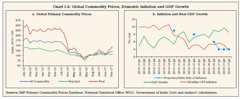 I.3 India’s moment of reckoning was no less cataclysmic. It arrived, not when it received legislative mandate in 2016, but back in the fateful summer of 2013 as the next section will etch out. Over the next three years, the RBI set about preparing the pre-conditions for the regime shift, learning from country experience, cherry picking the best practices from what worked and where. The journey was arduous, fraught with pitfalls of intellectual scepticism, including among practitioners (Reddy, 2008; Gokarn, 2010; Mohan, 2011; Ahluwalia, 2014; Subbarao, 2016; Jalan, 2017). Yet impossibly, the gods smiled and showered down encouragement in the form of a slump in international commodity prices (Chart I.2a) in those early years to help: after all, fortune favours the brave! Bracing up against the foreboding views of the orthodoxy, the transition to FIT was achieved by minimising the losses of output that typically take their toll in these regime changes (Chart I.2b). I.4 In 2016, it was heralded as India’s most successful structural reform of recent times5 and was subsequently endorsed by the IMF (Bauer, 2018). With influential voices of approval from academia and practitioners alike, the silent revolution is complete (Box I.2). I.5 With inflation aligned with the target over the period of FIT so far, i.e., 2016-17 to 2019-20 (excluding the period of the COVID-19 which saw severely distorted macroeconomic outcomes) and remaining below the emerging market and developing economies’ (EMDEs’) average and growth outperforming the latter, India engages with the global economy with the confidence of price stability (Chart I.3). The new kid on the FIT block has arrived. Yet, in spite of good luck and proactive preparation, the formal launch of FIT in September 2016 turned out to be what has been evocatively described as a ‘baptism by fire’ (Patra, 2017). Box I.2
Evolution of Ideas on Inflation Targeting in India Flexible inflation targeting (FIT) is closing on to turning five years old in India. The first monetary policy committee (MPC) completed its term in September 2020 and a new committee was notified in the Gazette of India on October 5, 2020. In its first meeting, the new MPC voted unanimously to maintain status quo on the policy rate and the stance as set out by the previous committee, thus preferring continuity. Early misgivings about ‘failure to launch’ – FIT being neonate, difficult to deliver, and blinkered – have waned and an eclectic debate, informed by its performance, has coursed through news media and academic papers, throwing up a rich diversity of views on its prospects. In the net, the MPC turned out to be dovish, to use the ornithological term preferred in the media. It delivered 250 basis points of rate cuts. Its stance was accommodative in 10 meetings, neutral in 12 and there were only two meetings in which it adopted a stance of ‘calibrated tightening’. Even so, initial views were that India’s underemployment and indebted firms whose balance sheets were sensitive to high interest rates warranted lower real rates at a time when globally, natural rates were at or tending to zero. In this line of argument, it was posited that the MPC ‘severely’ overestimated both inflation and future growth, and it was not until its February 2018 meeting that flexibility in FIT was utilised to nurture growth. This imposed a larger than necessary output sacrifice on the economy (Goyal, 2018; Mohan and Ray, 2019). Accordingly, a weighted average of five forecasts by market analysts, academics and government agencies with the best past performance was recommended along with the institution of formal reporting to Parliament to increase accountability. An asymmetric band of +3 and -1 per cent around the 4 per cent target – defined as core inflation – was called for, with equal weight to inflation and growth if the former is within the band (Goyal, op. cit.). Monetary policy impulses lost in transmission (Mohan and Ray, op. cit.) on account of the structural presence of the large impact of food prices on inflation dynamics were flagged against the backdrop of a long history of unstable prices and drifting inflation expectations as specific challenges confronting FIT in India (Al-Mashat, et al., 2018). On the other hand, estimates from a dynamic stochastic general equilibrium model indicated a strong transmission of monetary policy – especially from large interest rate changes – to output, inflation and interest rates even in comparison to the US, warranting milder monetary policy actions in response to supply shocks (Goyal and Kumar, 2019). It was believed, though, that inflation forecast targeting can provide an effective strategy for minimising the second round effects of supply shocks by stabilising long-term expectations as the central bank earned credibility over time by achieving the announced target for inflation. To buttress the credibility bonus, the publication of a forecast showing a conditional medium-term path of inflation falling back to target along with an explanation of how policy actions should contribute to this desired outcome was advocated (Al-Mashat, et al., op. cit.). Indeed, this suggestion was assiduously embraced and, along with the 12 months ahead forecast in the MPC’s resolution and the 18-24 months ahead forecast in the monetary policy report, considerable attention was given to unravelling the deviations of outcomes of both inflation and growth from forecasts; however, likely policy actions to align actual outturns in the future with the target were not explicitly provided and were instead embedded in the stated stance of the MPC at each meeting. It was recognised in the narrative around the FIT’s functioning that the assessment of the likely size and duration of each price event presented a monetary policy communication challenge (Al-Mashat, et al., op cit.). Nonetheless, delay in responding to supply shocks can be costly in terms of output losses and inflation, and hence assertive policy responses were advocated, in contradiction to arguments that the aggregate demand channel in India was strong and aggressive tightening could result in overreaction and overshooting in terms of output losses (Goyal, et al., op. cit.). By 2019-20, the final year of the first MPC, however, a combination of good luck and good policy had kept inflation aligned with the target with rare occasions of deviations beyond the band, and this turned the tide of opinion. Contrary to conventional wisdom, it was found that food inflation can un-anchor expectations, spillover into core inflation and hence warranted an appropriate monetary policy response rather than benign ‘looking through’. This result reinforced the choice of headline inflation as the appropriate inflation metric for India. Also contrary to the earlier mainstream, it was found that instead of neglecting output fluctuations, the RBI had diligently pursued FIT and was as responsive to output fluctuations as in the pre-FIT period (Eichengreen et al., 2020). An optimal policy rule with the ratio of weight on output gap to inflation gap higher than in the standard Taylor rule and a flexible inflation targeting framework turns out to be welfare maximising for India (Patra et al., 2017). The novelty in the RBI’s approach under FIT was a lower responsiveness than before to actual movements in inflation, suggesting forward-looking behaviour which enhanced policy credibility – smaller changes in the policy rate are now needed to signal the central bank’s intent (Eichengreen, op cit.). This bore out the empirical finding that inflation expectations, especially those of professional forecasters6, have become better anchored in India and inflation outcomes have become more stable, with lower volatility in the exchange rate and short-term interest rates. This has enhanced the ability of the RBI to respond to an exceptional shock like COVID-19 that is not of the authorities’ own making. This led up to the view that inflation targeting and its institutional arrangements had a payoff in terms of policy credibility and room for manoeuvre. Attention also turned to the institutional architecture as FIT matured in India. Justification has also been offered for decisions by an MPC (Dua, 2020). The growing prominence of the committee approach towards the conduct of monetary policy has several advantages, including confluence of specialised knowledge and expertise on the subject domain, bringing together different stakeholders and diverse opinions, improving representativeness and collective wisdom. The RBI’s monetary policy communication seems to have improved significantly with the advent of inflation targeting (Mathur and Sengupta, 2020). Comments on monetary policy in the media by some officials of the ministry of finance were seen as creating a public perception of lack of coordination. A government non-voting member could be a way to coordinate, but it was emphasised that the government needs to be cautious in not conveying the impression of interference or compromising the independence of the central bank (Patnaik and Pandey, 2020). In fact, this is important in a situation where two internal members of the MPC and all three external members are already appointed by the government. Publication of transcripts of monetary policy meeting with sufficient time lags were called for to improve transparency, with staggered terms for MPC members to guard against short-term political influences and to foster renewal of views. This public discourse has come full circle more recently in response to the incisive question that is in a fundamental sense the DNA of the future of FIT in India: Does the focus on inflation targeting mean a neglect of other objectives such as growth and financial stability? (Rangarajan, 2020). Correctly, this influential view argues that when inflation goes beyond the comfort zone, the exclusive concern of monetary policy must be to bring it back to the target. When inflation is within the comfort zone, authorities can look to other objectives. This is the essence of FIT – the objective of control of inflation is not independent of the objective of growth, and this is enshrined in the amended RBI Act. That is why the inflation mandate must provide for a range and a time frame for adjustment. While monetary policy must act irrespective of what triggers inflation, supply side management in situation of supply shocks should be the responsibility of the government. FIT is not a rule but a framework (Bernanke and Mishkin, 1997). In terms of the operating procedure, central banks wielding the short term interest rate as the instrument to achieve the objectives of inflation and growth act on liquidity so that the proposed policy rate change ‘sticks’. While the RBI must choose an appropriate measure of liquidity, this view held that the focus must also be on durable liquidity as reflected in reserve money (Rangarajan and Samantaraya, 2017). In terms of the inflation metric, it is better to deal with headline inflation with a range rather than excluding certain items (Rangarajan, 2020 op cit.). Monetary policy is ultimately the art or science of the feasible (Patra, 2017). Decision making is always complex and testing. The endeavour of the MPC is to undertake a balanced assessment and set it out before the public so that monetary policy in India becomes transparent and predictable. References: Al-Mashat, R, K. Clinton, D. Laxton, H. Wang (2018), “India: Stabilizing Inflation” published in the book Advancing the Frontier of Monetary Policy edited by T. Adrain, D. Laxton and M. Obstfeld, IMF eLibrary, April. Bernanke, Ben S. and Frederic S. Mishkin (1997), “Inflation Targeting: A New Framework for Monetary Policy?”, NBER Working Paper 5893, January. Dua, P. (2020), “Monetary Policy Framework in India”, Indian Economic Review (2020) 55:117–154, June. Eichengreen. Barry, Poonam Gupta and Rishabh Choudhary (2020), “Inflation Targeting in India: An Interim Assessment”, NCAER India Policy Forum 2020, July. Goyal, A. (2018), “Demand-led Growth Slowdown and Inflation Targeting in India”, Economic and Political Weekly, Vol LIII No. 13, March 31. Goyal, A. and A. Kumar (2019), “Overreaction in Indian Monetary Policy”, Economic and Political Weekly, Vol. LIV No. 12, March 23. Mathur, A. and R. Sengupta (2020), “Analysing Monetary Policy Statements of the Reserve Bank of India”, IGIDR WP-2019-012, April. Mohan, Rakesh and Partha Ray (2019), “Indian Monetary Policy in the Time of Inflation Targeting and Demonetization”, Asian Economic Policy Review, Volume 14, Issue 1, January. Patnaik, I. and R. Pandey (2020), “Moving to Inflation Targeting”, NIPFP Working Paper Series No. 316, 11 August. Patra, M. D., J.K. Khundrakpam and S. Gangadaran (2017), “The Quest for Optimal Monetary Policy Rules in India”, Journal of Policy Modelling, Volume 39, Issue 2, March-April. Patra, Michael D. (2017), “One Year in the Life of India’s Monetary Policy Committee”, Speech at the Jaipur Regional Office of the Reserve Bank of India, Jaipur, 27 October, published as BIS central bankers’ speeches at https://www.bis.org/review/r171123e.pdf. Rangarajan, C. (2020), “The New Monetary Policy Framework: What it Means”, Journal of Quantitative Economics, Springer, The Indian Econometric Society (TIES), Vol. 18(2), June. Rangarajan, C. and A. Samantaraya (2017), “RBI’s Interest Rate Policy and Durable Liquidity Question”, Economic and Political Weekly, Vol. 52, Issue No. 22, 3 June. | I.6 This chapter chronicles India’s formative experience with FIT in order to set up the laboratory for a review of the monetary policy framework, which is the theme of this year’s report. In what follows, an overview of the initial conditions and the impetus for change is set out in Section 2, followed in Section 3 by the experience of establishing the pre-conditions for ushering in FIT in India. The experience with de jure FIT since 2016 is assessed in Section 4. In these rites of passage, existential questions emerged, each of which forms the subject matter of dedicated chapters that follow. This chapter scheme is presented in Section 5, which concludes this chapter. 2. Initial Conditions I.7 The story of the monetary policy regime change in India to FIT goes back to the turbulent days of the global financial crisis (GFC). Reminiscent of 2018-20 (pre-COVID), the economy was into a three-quarter cyclical downturn before the GFC struck. The tide of the Great Moderation had lifted all boats across the world at the turn of the century. In India, real GDP growth averaged 7.9 per cent during 2003-08, peaking at 8.1 per cent in 2006-07. From Q4:2007-08, however, signs of the imminent slowdown began to show, and in the first half of 2008-09, growth slid to 7.4 per cent (at 2004-05 base). On this slope, the Lehman Brothers moment arrived and the world was consumed by the GFC, which has drawn parallel with the Great Depression of the 1930s – in fact, it has been termed as the Great Recession (Verick and Islam, 2010). India became a bystander casualty – in the second half of 2008-09, the slowdown became more pronounced and growth collapsed to 3.1 per cent for the full year. I.8 Cut to Circa 2009. India was among the first nations to bounce back from the GFC on the wings of a fiscal stimulus of 3.5 per cent of GDP7, a cumulative policy rate reduction of 425 basis points8 and assured liquidity of 10 per cent of GDP. The rebound took growth in 2009-10 to a level (7.9 per cent), higher than in the pre-GFC year of 2007-08 (7.7 per cent) even as the global economy contracted in 2009 (Chart I.3b). The momentum provided by the unprecedented stimulus measures pushed growth even higher in 2010-11 (8.5 per cent). Aspirations of India’s underlying potential seemed within reach, exemplified in official expectations of a growth rate of 9 per cent in 2011-129. The 12th five-year plan envisaged average growth of 8 per cent for the period 2012-17 on the back of a massive push to build a world class infrastructure, with the banking sector intermediating its financial requirements. 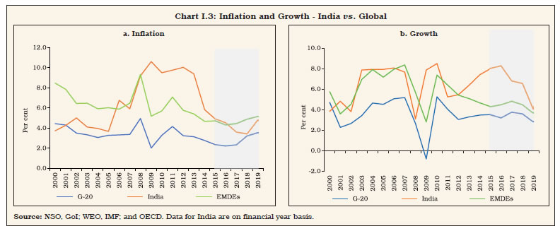 I.9 History would, however, ordain otherwise – 2009-10 would turn out to be a fateful year in the recent history of the conduct of monetary policy in India. First, the large monetary stimulus was not unwound in a timely manner. The RBI’s Annual Report for the year acknowledged that exit was debated in the light of the build-up of domestic inflationary pressures and inflation expectations. Clairvoyantly, it noted that the lag with which monetary policy operates pointed to a case for tightening sooner rather than later as the large overhang of liquidity could engender inflation expectations and an unsustainable asset price build-up, especially as capital inflows had resumed (RBI, 2010) (Chart I.4a). Eventually, however, arguments for deferring the unwinding won on the grounds of nurturing nascent growth impulses and also the facile view that inflationary pressures were driven by supply-side constraints, particularly food prices, which lie outside the remit of monetary policy (Chart I.4b). Exit did begin in October 2009, but it consisted of terminating some sector-specific liquidity facilities which were largely unutilised, restoring the statutory liquidity ratio (SLR) to its pre-crisis level [25 per cent of net demand and time liabilities (NDTL)], and restoring provisioning requirements for advances to the commercial real estate sector. Substantive liquidity withdrawal commenced from January 2010 when the cash reserve ratio (CRR) was raised by 75 basis points, but by then inflation was about to break out into double digits and race out of control. 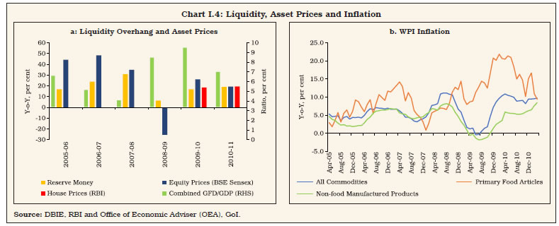 I.10 Second, confronted with conflict among its multiple objectives, the RBI leaned towards supporting growth, even at the cost of accommodating inflation – “there were definitive indications of the economy reverting to the pre-GFC growth trajectory” (RBI, 2010). Growth projections were strongly influenced by high frequency indicators, notably the index of industrial production (IIP) based to 1993-94. In terms of this index, growth surged from Q2 and rapidly accelerated into double digits in the second half of the year. By contrast, the new IIP series rebased to 2004-05, which became available in November 2011, showed that a tenuous recovery from contraction in Q1:2009-10 occurred in Q2 and Q3, and it was not until Q4 that a strong expansion started (Chart I.5). In hindsight, the RBI was carried away by the nation-wide robust optimism about growth aspirations that characterised those halcyon days and refrained from acting counter-cyclically. This would prove to be a costly policy error in terms of the original sin of time inconsistency, as subsequent inflation developments would reveal. 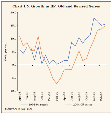 I.11 Third, the amphitheatre shifts to inflation and several lessons emerge. Measured by the then RBI’s metric – the wholesale price index (WPI) – prices emerged out of deflation in August 2009 but by December, it acquired elevation and persistence. The 2009 experience showed that it is crucial to carefully analyse the sources of inflation before making the judgment call on tolerating supply-side developments. Primary food prices had been ruling in double digits from as early as October 2008 and the failed monsoon of 2009 only stoked these pressures, taking food inflation to 20 per cent by December 2009. The signals being transmitted by food prices were set aside by design. In India, it is food (primary and manufactured combined) inflation which assumes properties of the true core when it persists, constituting 27 per cent of the old WPI index (1993-94=100) and a fourth of the 2004-05 based index which was released in September 2010. In the consumer price index (CPI) that is now the inflation metric, it’s share is 45.9 per cent. In fact, a benign neglect of the warning signs flashing from the CPI proved to be monetary policy’s costly error. In terms of the CPI for industrial workers (CPI-IW), food inflation had crossed into double digits by Q1:2008-09 itself and by Q3:2008-09 it had become generalised and spilled over into non-food components, taking headline inflation to 10.2 per cent in that quarter. Thus, although signals from both the WPI and the CPI were available to the RBI, they were looked through (Chart I.6a). Moreover, food inflation has a dominant influence on inflation expectations – in Q3:2009-10, households’ median inflation expectations (IE) a year ahead rose by 500 basis points to 13.5 per cent (Chart I.6b). Food inflation also exhibits a closer association with underlying demand than other exclusion-based measures of the core. The ‘official’ measure of core – non-food manufactured products inflation – was in deflation between April 2009 and October 2009, but this mainly reflected the weakness in international crude prices rather than a deficiency of demand since real GDP growth had regained mojo by Q2:2009-10. 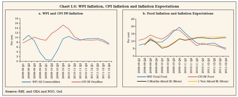 I.12 The spillover of food and fuel prices to non-food non-fuel inflation in WPI can be vividly illustrated by the historical decomposition of non-food non-fuel WPI inflation, which reveals the spillovers of elevated food inflation to non-food non-fuel inflation during 2009-10 (Chart I.7)10. This, in turn, led to generalised inflation during 2011-13. Thus, food price spillovers in an accommodative low interest rate regime led to unanchoring of inflation expectations ‘mutating like a multi-headed Hydra’ (Patra, 2017 op cit.). Over the period 2010-13, WPI headline inflation averaged 8.6 per cent. The sectoral CPIs were flashing red way ahead of the WPI. In 2009-10, inflation measured by the CPI-IW had risen to 12.4 per cent and averaged 9.7 per cent during 2010-13. 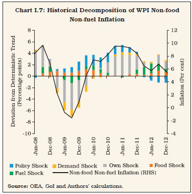 I.13 Between March 2010 and October 2011, the RBI raised its policy rate by 375 basis points in 13 consecutive actions, backed up by another CRR increase in April 2010 and the unwinding of all the extraordinary GFC liquidity measures in 2010 (Chart I.8). But inflation had checked in and it was there to stay, ‘all the king’s men and all the king’s horses’11 notwithstanding. And now, a more sinister drama was about to unfold. 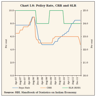 I.14 What if the RBI had behaved differently and the CPI inflation metric was used for policy? In order to assess this counterfactual, it is assumed that the RBI was operating in a rule-based policy environment with the objectives of attaining low and stable inflation and stabilising output. To simulate this scenario, a Taylor-type policy rule12 is estimated on quarterly data from 2000-01 to 2010-11 under the following heroic assumptions: i) the inflation target is set at 5 per cent; ii) the RBI follows interest rate smoothing like other central banks to avoid delivering monetary policy shocks, and adjusts its policy rate at a pre-announced quarterly frequency in sync with quarterly policy meetings; and iii) the weighted average call money rate (WACR) is used as the effective policy rate as the RBI did not use a single monetary policy instrument during that period. I.15 The inflation gap turns out to be statistically significant. The significance of the output gap coefficient and its larger size in comparison with the coefficient on inflation suggests that the RBI was more mindful of the growth objective relative to inflation13 (Table I.1). In fact, the stated view was that growth, price stability and financial stability formed a hierarchy of policy objectives with one or the other ascending the hierarchy depending on the underlying macroeconomic and financial conditions (Reddy, 2005). I.16 Given the large difference between WPI and CPI inflation during that period, a counterfactual analysis is conducted to assess whether the use of the CPI as the inflation metric would have evoked a different policy response. The Taylor-type rule suggests that if CPI-IW had been used as the primary inflation metric during 2009-2011, then it would have warranted a faster policy tightening after the GFC induced monetary policy accommodation (Chart I.9). Table I.1: Monetary Policy Reaction Function
(2000-01 to 2010-11) | | Smoothing Parameter | Inflation Gap$ | Output Gap^ | | 0.78*** | 0.41* | 0.75** | $ Deviation of WPI inflation from 5 per cent.
^ Estimated using Hodrick-Prescott (HP) filter.
***, ** and * represent significance at 1 per cent, 5 per cent and 10 per cent, respectively.
Source: Authors’ estimates. |
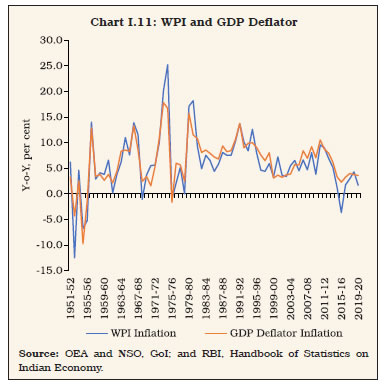
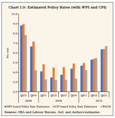 I.17 Looking back, the policy response was delayed. A timely response to a persisting supply shock is essential for a credible monetary policy. The more the delay, the costlier it will be for the economy. The importance of timely policy action can be shown with a policy experiment using the quarterly projection model (QPM)14 that formed part of the Forecasting and Policy Analysis System (Benes et al., 2016a) which has been developed as a precondition of the move to FIT in India. Defining steady state values of key macroeconomic parameters as a 5 per cent inflation target and 1.0 per cent as the real neutral rate (this is assumed based on the macroeconomic conditions prevailing during 2001-2011), the simulations show that there was a delay of four to six quarters in policy action, which kept the policy rate lower by up to 1 percentage point at its peak, i.e., Q3:2009 (Chart I.9). This led to an erosion of the central bank’s credibility, leading to unhinging of inflation expectations. As a result, inflation rose by 0.8 percentage point more than it would have, had there been no delay. Eventually, the RBI was forced to increase the policy rate by 1.5 percentage points more than what would have been needed in the case of a timely response. Also, the delay forced the RBI to keep the policy rate elevated for a longer period of time than warranted in a no delay case. This higher and more persistent policy response caused by the delay led to the output losses being larger (Chart I.10). Thus, the initial gains in output due to a delay in the policy response were eroded by the higher than warranted policy reaction later on, eventually resulting in a substantial deterioration in the medium-term output-inflation trade-off. I.18 Monetary policy is intrinsically a contract between the people and the sovereign. The people relinquish to the sovereign (or its agent, the central bank) the right over the value embodied in the goods and services they produce. In exchange, the sovereign undertakes to give to the people a money they can trust, a money that does not lose value over time in terms of the purchasing power it commands. Inflation is the metric by which this contract can be evaluated. Rising inflation erodes the purchasing power of money domestically, and externally as well by causing the exchange rate to depreciate against currencies of other countries that maintain a relatively lower rate of inflation. On the other hand, the inflation rate is also the rate of return on the production of goods and services. Too low a rate will disincentivise people from producing goods and services, thereby undermining the contract of trust. The challenge before the sovereign is to give to the people an appropriate inflation rate that balances these conflicting pulls and maximises social welfare. History has demonstrated that a break-down of this contract has severe repercussions, including the overthrow of sovereigns and the debasement of the currencies that circulate by their fiat. In India, a societal intolerance to inflation in high reaches and certainly at the double-digit threshold has manifested itself vividly – inflation measured by the GDP deflator and the WPI has averaged 6.4 per cent and 6.1 per cent, respectively, since 1951-52 (Chart I.11). Even short episodes of inflation beyond this social tolerance frontier are unacceptable, as election outcomes in India have repeatedly shown. In this fundamental sense, inflation is an index of governance (Patra, 2017 op cit.). I.19 The inflation experience of the immediate post-GFC years left deep scars on the economy. When inflation surged from 3.8 per cent in 2009-10 to 9.6 per cent in 2010-11 and it was seen to be accommodated by monetary policy in the year before, the credibility of the social contract came under scrutiny. Rates of returns on bank deposits adjusted for inflation turned negative ((-) 1 per cent). Meanwhile, real rates of return on alternative assets such as housing (about 10 per cent), equity (about 10 per cent) and gold (12.5 per cent) looked lucrative and induced a portfolio shift from financial assets to physical assets (Chart I.12a). Households’ financial saving declined from a recent peak of 10.9 per cent of GDP in 2009-10 to 7.4 per cent by 2011-12, with a corresponding increase in their physical assets from 14.0 per cent to 16.3 per cent (Chart I.12b). The rate of India’s gross domestic saving in which households are the prime movers (accounting for over 60 per cent) was at 36.9 per cent of GDP in 2010-11, but it underwent a prolonged decline that took it down to 30.6 per cent by 2018-19, before showing an uptick in 2019-20. 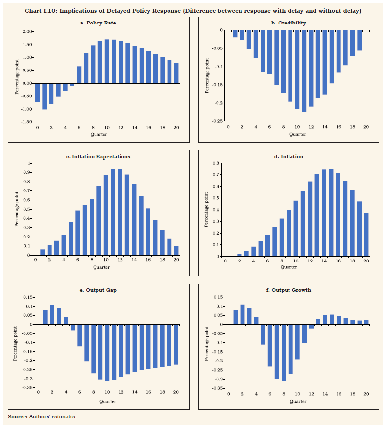
 I.20 In an apparent contradiction of the Feldstein-Horioka puzzle which suggests close correlation between domestic saving and investment, India’s gross domestic investment rate held up through these troubled times at around 39 per cent of GDP. With public investment declining from 9.0 per cent of GDP in 2008-09 to 7.2 per cent in 2012-13 as the GFC fiscal stimulus was unwound, the burden of sustaining the investment was entirely financed by foreign saving as reflected in the current account deficit (CAD) rising inexorably in those years from 0.1 per cent in Q4:2008-09 to a peak of 6.8 per cent of GDP in Q3:2012-13 (Chart I.13a). This was essentially reflecting a bad outcome. As people pulled out deposits from banks and bought gold, it reflected capital flight since India mines around one per cent of its gold consumption domestically. An annual level of gold imports of 750-850 tonnes surged to over 1000 tonnes in 2011-12 (Chart 13b). The RBI’s warnings on the CAD (RBI, 2012) went unheeded in the flush of large capital inflows which financed the unsustainable levels of the external financing requirement. 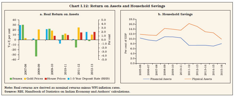 I.21 The moment of reckoning overwhelmed India in the summer of 2013 with the taper tantrum15. As financial markets reeled under high turbulence and risk-off sentiment became pervasive, capital flows stampeded for safe haven, exiting out of EMEs as an asset class. India was one of the worst hit, with the rupee depreciating the most among peers during May 22-August 30, 2013 (Chart I.14a). At that time, the foreign exchange reserves were close to US$ 300 billion, but markets discounted it completely (Chart I.14b). India joined Brazil, Indonesia, South Africa and Turkey in what was termed the ‘fragile five’16. An unconventional crisis defence had to be mounted. Liquidity operations ensured that the money market rates were tightened; foreign exchange reserves were augmented by overseas borrowings and swaps; and gold imports were restricted through both tariffs, and end use constraints17. Although the crisis was seen off and the situation stabilised thereafter, inflation had taken a heavy toll on macroeconomic conditions. With public credibility in monetary policy eroded, the time for regime overhaul was upon the RBI and India. 
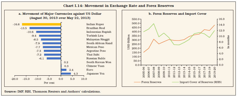 3. Preconditions I.22 In July 2013, a rare data point was formed – monetary policy was employed in defence of the exchange rate for the second time in recent history, the first being in the GFC. Facing risks of currency turmoil due to the taper tantrum, the RBI judged that spillovers could endanger financial stability and growth and gave priority to stabilisation of the rupee in the conduct of monetary policy (RBI, 2014). The easing phase in the monetary policy stance that had commenced in April 2012 in response to the growth slowdown, after the delayed tightening during 2010-2011 to fight inflation, was interrupted. A 200 bps hike in the marginal standing facility (MSF) rate was effected and was backed up by capping individual bank’s access to the liquidity adjustment facility (LAF) at 0.5 per cent of its NDTL, increasing the average daily CRR maintenance requirement (initially to 99 per cent from 70 per cent and thereafter to 95 per cent), and conducting open market sales to further tighten liquidity so that the MSF rate became the effective policy rate, 300 basis points above the de jure policy repo rate (Chart I.15). Although the exchange rate stabilised in ensuing months, inflation pressures persisted, warranting a more conventional monetary policy response in the form of policy rate increases in September and October 2013 even as the unconventional measures began to be wound down. Around this time, the RBI began setting the preconditions for a new monetary policy regime. 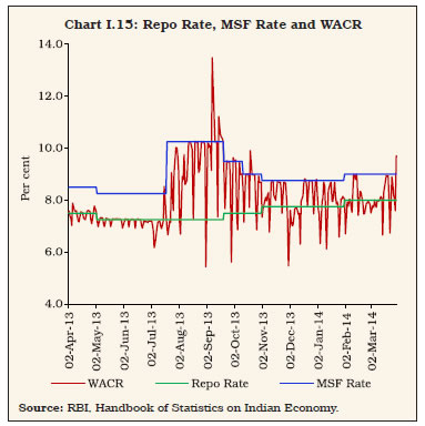 I.23 First, in September 2013, an expert committee was appointed to revise the monetary policy framework within a five-pillar approach comprising clarifying and strengthening the monetary policy framework, strengthening the banking structure, broadening and deepening financial markets, fostering financial inclusion, and improving the system’s ability to deal with financial stress (RBI, 2014). The recommendations of this committee on the choice of a nominal anchor for monetary policy, decision making, instruments and operating procedure, transmission and open economy monetary policy provided the intellectual edifice for fashioning the new regime. This is detailed in Chapter 4. I.24 Second, inflation was chosen as the nominal anchor for monetary policy in India in January 2014, drawing on the Committee’s recommendations and the wider country experience. Well ahead of formal adoption, the RBI began sensitising the public about the choice of metric for the nominal anchor as this would involve a shift from the WPI to the CPI18. From the October 2013 monetary policy review, retail inflation measured by the new CPI was analysed and projections in the form of fan charts were provided for the first time, effectively marking the beginning of the transition. Two challenges presented themselves. First, in the absence of any prior experience with CPI inflation, the RBI’s policy reaction function was indeterminate. Second, 46 per cent of the new index comprised food and beverages – as against 24 per cent of the WPI based to 2004-05 – rendering the inflation process volatile and prone to supply shocks over which monetary policy had no control. On the other hand, the CPI is internationally used to express inflation; it is also easily communicated and understood, being a measure of prices at the retail level facing households and hence driving the formation of their expectations. In the context of changes in food and fuel prices, therefore, the commitment to the nominal anchor would need to be demonstrated by timely and even pre-emptive policy responses to risks from second round effects in order to anchor inflation expectations. I.25 Understanding the nature and type of supply shocks is critical for calibrating monetary policy actions. Even though monetary policy cannot control these shocks, it can play an important role in avoiding the generalisation of inflationary pressures from the shock. Counterfactual experiments on food price shocks, i.e., (i) transitory shocks from vegetables prices; and ii) persistent shocks due to monsoon vagaries can be carried out by employing QPM – the RBI’s workhorse model (Chart I.16). In the case of a transitory food price shock, the initial price spike reverses, inflation falls, and monetary policy sees through the shock by not changing the policy rate [Chart I.16 (i.a, b, c)]. On the other hand, if monetary policy chooses to react to the transitory shock by increasing the policy rate, this will induce volatility in the output gap without having a discernible impact on the inflation path. A persistent food price shock warrants a monetary policy action to prevent un-anchoring of inflation expectations and spillover effects [Chart I.16 (ii.a, b, c)]. If monetary policy decides to see-through this shock, inflation expectations become unanchored, leading to a persistent upward drift in inflation, which does not fall back to the pre-shock level even after the initial shock has completely dissipated. I.26 Third, inflation measured by the CPI had reached a peak of 11.5 per cent in November 2013. Bringing it down to a more tolerable level was a formidable task, given the cross-country evidence that the costs of disinflation are substantial. In a cross-country setting, each percentage point decline in trend inflation costs about 1.4 percentage points of a year’s output (Ball, 1994), often termed the sacrifice ratio. Policy makers, therefore, often take a gradual approach as they fear that a deep recession could result from a ‘cold turkey’ approach or a sharp tightening of monetary policy. The RBI, too, avoided a ‘big bang’ and preferred a medium-term horizon of disinflation to minimise the associated output losses by spreading them over a multi-year time frame. A glide path was set up that would bring down inflation to 8 per cent by January 2015 and 6 per cent by January 2016 (RBI, 2014). In the event, tailwinds from a collapse of commodity prices enabled measured CPI inflation to ease to 5.2 per cent in January 2015 and 5.7 per cent in January 2016 (Chart I.17). 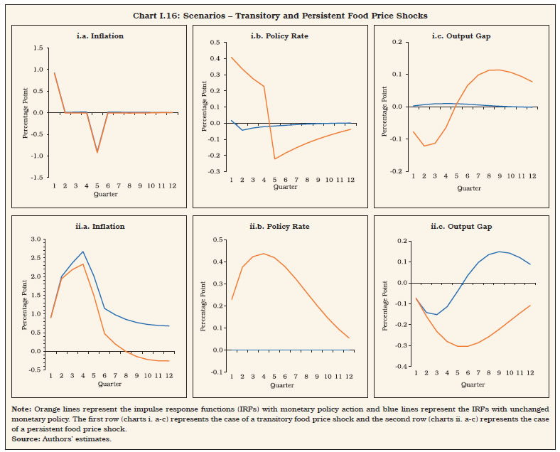 I.27 Fourth, after a hiatus of four years, the commitment to fiscal prudence was renewed. The union budget for 2012-13 set out a roadmap for fiscal consolidation by budgeting a reduction in the gross fiscal deficit (GFD) to GDP ratio beginning from 2012-13 and continuing the process through further corrections under rolling targets for the next two years. This was sought to be achieved through revenue enhancing (especially indirect tax measures and non-tax revenues through spectrum auction receipts) and expenditure control measures, viz., restricting expenditure on subsidies to below 2 per cent of GDP. The widening of the services tax base and a partial rollback of crisis-related reductions in various indirect tax rates also contributed to the tax receipts of the central government. 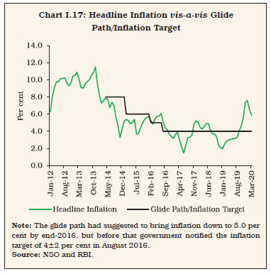 I.28 The amendment of the Fiscal Responsibility and Budget Management (FRBM) Act, 2003 in 2012 incorporated a medium-term expenditure framework statement (MEFS), which was a significant initiative towards fiscal consolidation. Under the amended FRBM Act, the government sought to eliminate the revenue deficit excluding grants for creation of capital assets by 2014-15, thereby targeting correction in respect of the structural component of the deficit in the revenue account. The MEFS set out three-year rolling targets for expenditure indicators as part of the strategy to improve the quality of public expenditure management. In response, the GFD of the centre declined from 6.6 per cent in 2009-10 to 4.1 per cent by 2014-15 (Chart I.18). I.29 Fifth, the external sector regained resilience and strength. Supported by terms of trade gains from the plunge in international commodity prices, the current account deficit declined from its annual peak of 4.8 per cent of GDP in 2012-13 to 0.6 per cent in 2016-17. By the end of 2016-17, resurgence of capital flows and a modest external financing requirement enabled the level of reserves to rise to US$ 370 billion, equivalent to 11.3 months of imports. The ratio of reserves to external debt rose from 71.3 per cent at the end of March 2013 to 78.4 per cent by end 2016-17 and the ratio of the net international investment position to GDP fell from 17.8 per cent to 16.8 per cent.  I.30 Sixth, the core of FIT is inflation forecast targeting. Consistent and reliable forecasts are prerequisites for the conduct of forward looking monetary policy under which the forecasts act as the intermediate target for monetary policy, a la monetary aggregates in the earlier regime. Hence, a theoretically consistent and empirically founded model, taking into account the specific characteristics of the Indian economy, was needed to be developed, especially in the context of external communication of inflation forecasts. In fact, Section 45ZM of the RBI Act mandates the RBI to publish a half-yearly Monetary Policy Report (MPR), including inflation forecasts for 6-18 months. It is in pursuance of this requirement that the RBI developed a macro economic model – QPM – under the Forecasting and Policy Analysis System (FPAS) for generating medium term projections and policy analysis19. QPM is a forward looking open economy calibrated gap model broadly following a theoretical framework founded on New Keynesian principles in the widely adopted tradition among modern central banks and consistent with meeting the targets/mandate set under the FIT regime (Benes et al. 2016a, b). It provides the flexibility to incorporate empirical regularities (Chart I.19). I.31 The QPM embeds key India-specific features like behaviour of different inflation components and their interlinkages, sluggishness in monetary policy transmission, the predominance of the bank lending channel, and credibility. It also incorporates monetary-fiscal linkages, fuel pricing, capital flow management and exchange rate dynamics. An innovative feature of India’s QPM is the incorporation of the credit constraint on output via the bank lending channel, which resolves the issue of extracting valuable information from monetary and credit aggregates that canonical New Keynesian models are criticised for. I.32 Fundamentally, the QPM is a framework designed to answer one question: what is the path of the policy rate, given the macroeconomic and financial conditions? The policy interest rate is endogenous and consistent with the inflation target. For any deviation of inflation from its target, however, there are many alternate interest rate paths that would bring inflation back to target over the medium term: for example, large early policy rate changes may get inflation to target quickly, but with a substantial adverse impact on output; more gradual policy actions will achieve the target slowly, but with less loss of output. Thus, this model can be calibrated to generate alternate interest rate paths, which are consistent with the inflation target, taking into consideration the policy makers’ assessments of evolving macroeconomic conditions.  I.33 Against this backdrop of milestones set and crossed during 2013-15, formal FIT in its de jure format was ushered in during 2016-17. Amendments to the RBI Act came into force on June 27, 2016. For the first time in its history, the RBI was explicitly provided the legislative mandate to operate the monetary policy framework of the country. The primary objective of monetary policy was also defined explicitly for the first time – “to maintain price stability while keeping in mind the objective of growth.” The amendments also provided for the constitution of an MPC that shall determine the policy rate required to achieve the inflation target, another landmark in India’s monetary history. The composition of the MPC, terms of appointment, information flows and other procedural requirements such as implementation of and publication of its decisions, and failure to maintain the inflation target as well as remedial actions were specified and subsequently gazetted during May-August 2016. On August 5, 2016 the Government set out the inflation target as four per cent with upper and lower tolerance levels of six per cent and two per cent, respectively, for a period of five years up to March 31, 2021. On September 29, 2016 a press release of the Government of India informed of the appointment of external members of the MPC. One working day later, the MPC began its first ever meeting and issued its first unanimously voted resolution on October 4, 2016 (Table I.2). The specific dates and events around establishment of FIT in India suggest that the objective was to facilitate a smooth transition to minimise output losses. 4. Experience with FIT I.34 With the formal institution of FIT in September 2016, India became the 36th country to adopt an inflation targeting monetary policy regime (Jahan, 2017) – the new kid on the block – and as stated in the foregoing, with many ‘firsts’ to its credit. The fortunes of FIT and India’s first MPC were intertwined over a tumultuous period by any reckoning. The latter held 24 meetings in total, including two off-cycle. I.35 Ahead of its first meeting, CPI inflation was on the decline from a recent peak, enabling the MPC to begin its innings with a unanimous rate reduction of 25 basis points and an accommodative stance. In its next meeting, however, FIT/the MPC had to deal with its first unforeseen shock that was domestic in character – demonetisation. Deflationary forces took hold, bringing headline inflation to an all-time low of 1.5 per cent in June 2017, below the lower tolerance level. Meanwhile real GDP growth moderated and slowed sequentially to 5.8 per cent in Q1:2017-18. Towards the close of the tenure of the MPC, i.e., from March 2020, FIT was tested again by an unprecedented and equally unforeseen shock but of global proportions this time – COVID-19. Pre-emptively, the MPC met off-cycle and effected the biggest rate cuts in its lifetime – 115 basis points cumulatively during March-May – and nuanced its accommodative stance to incorporate the resolve to “mitigate the impact of COVID-19 on the economy” (RBI, 2020), in spite of inflation having breached the upper tolerance level during December 2019-February 2020. | Table I.2: Transition to FIT in India | | Date | Event | Outcome | | January 2014 | RBI announced a disinflationary glide path for bringing down CPI inflation to 8 per cent by January 2015 and to 6 per cent by January 2016. | Inflation fell in line with the glide path to 5.2 per cent in January 2015 and 5.7 per cent in January 2016. | | February 20, 2015 | A Monetary Policy Framework Agreement (MPFA) was signed between the Government of India and the Reserve Bank. | FIT was formally adopted in India with RBI tasked to bring inflation to 6 per cent by January 2016 and target for 2016-17 and all subsequent years shall be 4 + 2 per cent. | | February 29, 2016 | The Finance Minister announced in his Budget Speech for 2016-17 the Government’s intention to amend the RBI Act, 1934 to provide for a statutory and institutionalised framework for a Monetary Policy Committee (MPC). | The RBI Act 1934 was amended to provide statutory basis for a Monetary Policy Framework and a Monetary Policy Committee through the Finance Bill 2016. | | May 14, 2016 | Amendment to the RBI Act was notified in the Gazette of India. | Statutory basis to the FIT framework. | | June 27, 2016 | The amended RBI Act came into force on June 27, 2016. Rules governing the procedure for selection of members of MPC and terms and conditions of their appointment and factors constituting failure to meet inflation target under the MPC Framework notified. | Sought to ensure independence and accountability, MPC vested with the responsibility of setting the policy rate. | | August 5, 2016 | Under section 45ZA of the RBI Act, 1934, the Central Government, in consultation with RBI, fixed the inflation target for the period from August 5, 2016 to March 31, 2021, as 4 per cent, with upper tolerance level of 6 per cent and lower tolerance level of 2 per cent. | Fixation of an inflation target while giving due emphasis to the objective of growth and challenges of an increasingly complex economy is an important monetary policy reform with necessary statutory back-up. | | September 29, 2016 | Constitution of the MPC under section 45ZB of the RBI Act, 1934 notified. | Government constituted the six member MPC for the first time with (a) the Governor of the Bank as Chairperson, ex officio; (b) Deputy Governor of the Bank, in charge of Monetary Policy - Member, ex officio; (c) One officer of the Bank to be nominated by the Central Board - Member, ex officio; and (d) three external members – Professor Chetan Ghate, Professor Pami Dua and Professor Ravindra H. Dholakia. | | October 3-4, 2016 | The MPC held its first meeting. | Unanimous decision to reduce policy rate by 25 bps, consistent with the accommodative policy stance. | | October 5, 2020 | Government constituted a new MPC on the expiry of the term of the first MPC with three external members: Dr. Shashanka Bhide; Dr. Ashima Goyal; and Prof. Jayanth R. Varma. | The 25th meeting of the MPC was held from October 7 to 9, 2020 and members voted unanimously to keep the policy rate unchanged at 4.0 per cent, while deciding to continue with the accommodative stance as long as necessary. | | Source: RBI Annual Reports; PIB, Government of India; RBI Act, 1934 (amended). | I.36 Thus, the MPC/FIT had to deal with inflation variability of sizable amplitude and a unidirectional slowing down of growth in the downturn phase of the cycle. These subtle variations in situations and responses serve to underscore the ‘F’ of FIT, i.e., flexibility in the context of acute policy trade-offs. I.37 An abiding theme in the rapidly proliferating literature is to evaluate the performance of FIT against a variety of metrics (Ball and Sheridan, 2005; Fraga et al. 2003; Gonçalves and Salles, 2008; Mishkin and Schmidt-Hebbel, 2007). The main criteria for evaluating any policy regime are the specific objectives assigned to it. Macroeconomic Performance20 I.38 First, over the period October 2016 to March 2020 – the principal metric set by the Act, i.e., headline inflation averaged 3.9 per cent, even with the two life changing shocks alluded to earlier. Second, apart from aligning inflation with the target, the success of FIT lies in providing certainty to people about the course of future inflation by minimising its fluctuations. This is the crux of price stability. It is measured by the second moment about the mean, i.e., inflation volatility, measured by its standard deviation, declined to 1.4 during October 2016-March 2020 from 2.4 in 2012-16 (Table I.3). I.39 Third, people’s expectations are also influenced by how inflation outcomes are distributed, which is the third moment about the mean. If they are more above the mean than below, there is a negative or left-tailed skew, which implies that most of the time, people are likely to face higher than average inflation. On the other hand, when the distribution of inflation is positively skewed or right-tailed, people would generally expect lower than average inflation. During the period of FIT and the first MPC, skewness was 0.9, indicating that over most of this period, inflation was lower than the average. Fourth, kurtosis, the fourth moment about the mean, describes the proportion of inflation outcomes that are far away from the average. In the case of FIT, it was 0.9, implying that there were very few instances of large deviations from the mean. During 2012-16, for instance, it was (-)1.5. Taken together, skewness and kurtosis of the inflation distribution during FIT suggest that most outcomes for headline inflation were concentrated around the mean of 3.9 per cent. This is in contrast to the bi-modal distribution observed during 2012-16 (Chart I.20.a). I.40 During the FIT period, even the distribution of inflation across sub-groups was centred around the inflation target of 4 per cent as opposed to a wide range of outcomes in the pre-FIT period, as reflected in the long tails of the distribution during 2012-16 (Chart I.20.b). | Table I.3: Headline Inflation – Key Summary Statistics | | (Per cent) | | | 2012-13 | 2013-14 | 2014-15 | 2015-16 | 2012-16
(Apr-12 to Sep-16) | 2016-17 | 2017-18 | 2018-19 | 2019-20 | 2016-20
(Oct-16 to Mar-20) | | Mean | 10.0 | 9.4 | 5.8 | 4.9 | 7.3 | 4.5 | 3.6 | 3.4 | 4.8 | 3.9 | | Standard Deviation | 0.5 | 1.3 | 1.5 | 0.7 | 2.4 | 1.0 | 1.2 | 1.1 | 1.8 | 1.4 | | Skewness | 0.2 | -0.2 | -0.1 | -0.9 | 0.1 | 0.2 | -0.2 | 0.1 | 0.5 | 0.9 | | Kurtosis | -0.2 | -0.5 | -1.0 | -0.1 | -1.5 | -1.6 | -1.0 | -1.5 | -1.4 | 0.9 | | Median | 10.1 | 9.5 | 5.5 | 5.0 | 7.1 | 4.3 | 3.4 | 3.5 | 4.3 | 3.6 | | Maximum | 10.9 | 11.5 | 7.9 | 5.7 | 11.5 | 6.1 | 5.2 | 4.9 | 7.6 | 7.6 | | Minimum | 9.3 | 7.3 | 3.3 | 3.7 | 3.3 | 3.2 | 1.5 | 2.0 | 3.0 | 1.5 | Note: Skewness and kurtosis are unit-free.
Source: NSO and Authors’ calculations. |
Inflation Dynamics I.41 Pinning down the underlying inflation dynamics – sources of inflation; relative price movements; inflation persistence; and inflation expectations – is important for evaluating the FIT experience. Understanding regional or spatial inflation dynamics is significant in this exercise. (a) Sources of Inflation I.42 Beginning with the sources of inflation, the disinflation ahead of FIT was broad-based, but driven mostly by the food group (Table I.4). During FIT, the enduring alignment of inflation with the target was enabled by a sharp fall in food inflation under the impact of record food grains and horticulture production. Reliance on food imports declined (except for palm oil and some pulses) and consequently, the correlation of global food inflation with domestic CPI food inflation fell in the four years leading up to FIT (Chart I.21.a). Improvements in road network, tele-density, market penetration and irrigation facilities helped reduce multi-stage mark-ups over the food supply chain in India (Bhoi, et al., 2019). I.43 Sustained moderation in the growth of agricultural and non-agricultural wages played a role in containing food price inflation during the FIT period, and lower inflation also contributed to lower wage growth (Chart I.21.b). Food inflation volatility remained high through the FIT period, however, suggesting persisting vulnerability to supply shocks such as the vagaries of the monsoon and idiosyncratic price shocks as in pre-monsoon upticks. I.44 On the other hand, the volatility of core inflation – obtained by excluding food and fuel prices from the headline – more than halved during the FIT period. Positive spillovers from the sharp reduction in food inflation, a relatively stable exchange rate and the credibility bonus accruing to monetary policy on account of its focus on an inflation target contributed to this outcome. By contrast, the sharp reduction in international crude oil prices and their volatility did not fully pass through to domestic petroleum, oil and lubricants (POL) prices due to opportunistic fiscal revenue raising rather than consumption smoothing. In fact, global non-food primary commodity price inflation (consisting of fuel, metals, fertilisers and agricultural raw materials) exhibited high positive contemporaneous correlation with domestic CPI-core inflation during the pre-FIT and the FIT periods (Chart I.22). | Table I.4: CPI-C Inflation Components, Agricultural Growth and International Crude Oil Prices - Level and Volatility | | (Per cent) | | | Average | Volatility | | | Food and Beverages (45.9) | Fuel and Light (6.8) | Ex-Food and Fuel (Core) (47.3) | Agricultural GVA Growth | International Crude Oil Prices (USD/Barrel) | Food and Beverages | Fuel and Light | Ex-Food and Fuel (Core) | Agricultural GVA Growth | International Crude Oil Prices (USD/Barrel) | | Pre-FIT | | 2012-13 | 11.2 | 9.7 | 9.0 | 1.5 | 103.2 | 1.2 | 1.0 | 0.4 | 0.4 | 5.7 | | 2013-14 | 11.9 | 7.7 | 7.2 | 5.6 | 103.7 | 2.5 | 1.2 | 0.4 | 1.1 | 3.3 | | 2014-15 | 6.5 | 4.2 | 5.4 | -0.2 | 83.3 | 2.2 | 0.7 | 1.1 | 3.1 | 23.6 | | 2015-16 | 5.1 | 5.3 | 4.6 | 0.6 | 46.1 | 1.2 | 0.7 | 0.3 | 2.2 | 11.1 | | Period average | 8.7 | 6.7 | 6.5 | 1.9 | 84.0 | 3.4 | 2.3 | 1.8 | 2.7 | 27.0 | | FIT | | 2016-17 | 4.4 | 3.3 | 4.8 | 6.8 | 47.9 | 2.4 | 0.8 | 0.2 | 1.4 | 4.3 | | 2017-18 | 2.2 | 6.2 | 4.6 | 6.6 | 55.7 | 1.9 | 1.3 | 0.5 | 0.9 | 7.0 | | 2018-19 | 0.7 | 5.7 | 5.8 | 2.6 | 67.3 | 1.8 | 2.7 | 0.4 | 1.0 | 7.6 | | 2019-20 | 6.0 | 1.3 | 4.0 | 4.3 | 58.6 | 3.9 | 3.1 | 0.4 | 1.3 | 9.3 | | Period Average | 3.3 | 4.1 | 4.8 | 5.1 | 57.4 | 3.3 | 2.9 | 0.7 | 2.0 | 9.9 | Note: Volatility is measured by standard deviation of monthly y-o-y inflation of the CPI-C components, quarterly agricultural GVA growth and monthly average international crude oil prices. Petrol and diesel are part of transport and communication sub-group under core inflation. Figures in parentheses represent weights in per cent in CPI-C. Average volatility indicates standard deviation of the variable for the relevant full period.
Source: NSO, IMF Primary Commodity Prices database and Authors’ calculations. |
 I.45 An analysis of the relationship between core (excluding food, fuel, petrol and diesel) and non-core components of CPI suggests that non-core inflation converges to core inflation and the deviations from equilibrium gets corrected in around a year (Table I.5)21. The large residual volatility of non-core inflation (compared to core inflation) indicates the transitory nature of the non-core inflationary shocks. On the other hand, in the short-run, a positive relationship between non-core inflation and core inflation is found to be statistically significant, indicating that spillovers also happen from non-core inflation to core inflation through increased costs as well as unanchored inflation expectations. | Table I.5: Core and Non-Core Inflation Dynamics | | | ΔNonCore | ΔCore | | Error Correction Term | -0.069*** | 0.005 | | ΣΔCore | -0.637 | 0.231** | | ΣΔNonCore | 0.353*** | 0.075*** | | Residual SD$ | 0.607 | 0.164 | | Cointegration Test (F-Statistic) | 4.073* | 4.773* | | Residual White Noise Test (p-value) | 0.481 | 0.634 | ***, ** and * represent significance at 1 per cent, 5 per cent and 10 per cent, respectively.
$ The standard deviation (SD) corresponds to non-annualized m-o-m changes.
Note: In addition, a dummy variable to control for the increase in the housing inflation during January 2017 to June 2017 due to changes in sample process was used.
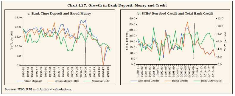
Source: Authors’ estimates. | (b) Relative Price Movements I.46 Monetary policy is concerned with the change in absolute level of prices as reflected in headline inflation; relative prices do not matter as they should be counterbalancing within the budget constraint. If relative prices are large, persistent and not offsetting, however, they impinge on the setting of monetary policy as they can influence inflation expectations lastingly through second-round effects. I.47 Relative food price, i.e., the ratio of food to non-food price indices, was trending up during the period from 2005 to 2014. With the de facto notification of FIT from 2014, relative food prices started to show signs of moderation (Chart I.23). A combination of successive record harvests, improvements in supply management and moderate increases in MSPs contributed to disinflation under FIT. This underscores the need for close coordination between the central bank and supply management authorities to achieve FIT optimally. (c) Inflation Expectations I.48 Under FIT, forward-looking monetary policy endeavours to anchor inflation expectations of households and businesses to the target so that they can make spending and investment decisions with reasonable certainty. Accordingly, they incorporate the target level of inflation into their wage and price-setting behaviour which, in turn, reinforces the probability of achieving the target in the future and hence, the effectiveness of monetary policy. It is in this context that inflation expectations form an essential input in the central banks’ policy framework (Shaw, 2019). In India, median inflation expectations of urban households over a one-year ahead horizon moderated to an average of 8.7 per cent during the FIT period from 12.5 per cent during the pre-FIT period. A host of other measures of inflation expectations in India such as those derived from surveys of consumer confidence, industrial outlook and professional forecasters reveal that inflation expectations of various economic agents are broadly aligned (please refer to Chapter 2 for details). Inflation expectations of private agents in the economy are, however, generally backward-looking, i.e., they are likely to be influenced by prices of salient items of consumption – such as food and fuel – today or a month or two ago. Consequently, monetary policy has to be sensitive to such shocks to prices of households’ consumption items so that they do not feed through into prices of other items and become generalised. The objective of monetary policy should, therefore, be to prevent inflation expectations developing inertia around high levels, underscoring the complementarity between aggregate demand and supply management policies. (d) Inflation Persistence I.49 Persistence can perhaps be likened to inertia in physics – the resistance of a body to changing its velocity unless acted upon by an external force (Fuhrer, 2010). A more formal definition of inflation persistence is “the tendency of inflation to converge slowly to its long-run value following a shock” (Altissimo et al., 2006). Understanding the speed and manner in which inflation adjusts to shocks of varying nature, and measuring the patterns and determinants of inflation persistence, is critical for fashioning the monetary policy response to upsurges in inflation – reacting heavy-handedly to shortlived episodes can lead to overkills of economic activity; by contrast, too delayed or too feeble a response to long-lasting inflation occurrences runs the risk of hardening inflation expectations and entrenching them at elevated levels with harmful effects that can even impair potential growth (IMF, 2011). While the size and timing of monetary policy reactions are eventually judgement calls, empirical measurement of inflation persistence can shine light on the judgement process. Furthermore, this has to be country-specific since the characteristics of the economy in question play a determining role in the dynamics of inflation (Patra et al., 2014). In India, inflation persistence was found to be lower during the FIT period (please refer to Chapter 2 for details). Thus, the cost of correcting deviations of inflation from the target by monetary policy action diminishes going forward. (e) Regional Inflation Dynamics I.50 Although the inflation target in India is defined in terms of headline inflation, regional inflation dynamics cannot be overlooked, as that may constrain a nationally set monetary policy in adequately satisfying the needs of all regions (Beck and Weber, 2005; Weyerstrass et al., 2011). While the data reveal wide dispersion in inflation across states driven largely by food prices, state level inflation tends to converge towards national inflation in India (Kundu et.al., 2018) – the recent stability in both the mean inflation differential and inflation differential volatility validates this convergence (Chart I.24a). Furthermore, the estimated kernel density plot of deviations of state level inflation from national inflation during 2012-13 to 2019-20 is more or less symmetric, reinforcing the evidence on convergence (Chart I.24b)22. 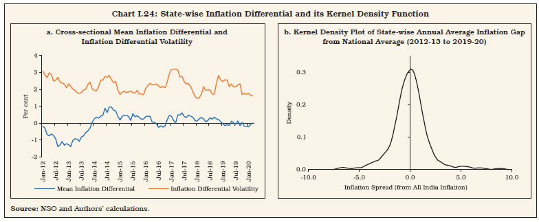 I.51 As India is characterised by sizable differences in income levels, agro-climatic conditions, population characteristics, and levels of industrialisation and urbanisation, it is also important to test for the existence of a long-run equilibrium relationship between rural and urban inflation. It is observed that rural inflation eased till 2018-19 before picking up, while urban inflation moderated a year earlier and picked up thereafter (Chart I.25a). At a disaggregated level, the divergence between rural and urban inflation in recent years largely mirrors the divergence in the behaviour of food inflation, urban being higher than rural (Chart I.25.b). Empirical evidence suggests a long-run co-integrating relationship between urban and rural inflation with deviations adjusting to long-run equilibrium within 2-3 quarters23. 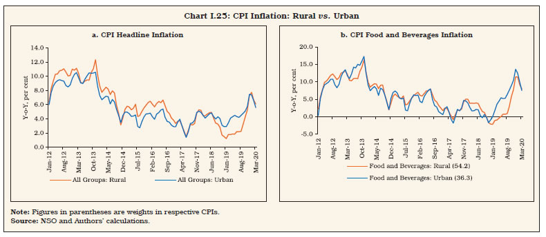 I.52 In sum, these findings suggest that irrespective of short-run divergences, monetary policy could rely on the all-India level headline inflation (Bhoi et al., 2020). This validates the choice of national level CPI (headline) inflation as the nominal anchor for monetary policy under the FIT regime in India. Growth Dynamics I.53 How has FIT measured up in terms of its secondary objective: “keeping in mind the objective of growth”? Average real GDP growth at 6.0 per cent during the FIT period (Q3:2016-17 to Q4:2019-20) was lower by 1.1 percentage points than in the pre-FIT period (Q1:2012-13 to Q2:2016-17). The pre-FIT period was characterised by one of the longest cyclical upswings in the post-independence era, with real GDP growth peaking at 9.7 per cent in Q2:2016-17. Robust growth in the industrial and services sectors was supported by a rebound in agriculture after two consecutive years of droughts. From 2017-18, a cyclical downturn set in, delayed in the second half of the year by favourable base effects. From the beginning of 2018-19, real GDP growth moderated sequentially for eight consecutive quarters in sync with the global slowdown. Increasingly, countries across the advanced and emerging worlds joined the synchronous global deceleration, the coupling accentuated by geopolitical developments, trade wars, and idiosyncratic factors like emission norms. Domestic factors like stress in the balance sheet of corporates and financial institutions, inventory overhang in the real estate sector, and unfavourable terms of trade sapped real GDP growth in India, taking it down to 3.1 per cent in Q4:2019-20 – the lowest in the 2011-12 series. I.54 India’s growth slowdown during the period of FIT was also associated with a weakening in the pace of trend growth24 (Chart I.26 a). It co-moved with a downturn in saving and investment rates, a prolonged deceleration in manufacturing, a decline in openness and diminishing returns of the demographic dividend. All these factors were being reflected in a weakening of monetary and credit aggregates. Thus, the question of low and stable inflation in India during FIT not being associated with higher growth has to be addressed by investigating the structural changes underway in the Indian economy. I.55 The deceleration in India’s trend growth started in 2008-09 following the GFC, obscured by the massive (fiscal and monetary) policy stimulus holding up growth in saving and investment rates (Chart I.26 b). This was in contrast with the significant rise in domestic saving from 2003-04, which enabled an increase in the investment rate up to 2007-08. During this upswing, however, the behaviour of household savings was unusual – despite the strong pace in financial innovations, there was a continued preference for saving in physical assets, which prolonged until 2011-12. The consequent decline in the financial saving rate (especially in bank deposits) by households resulted in a deceleration in money growth, bank credit growth and GDP growth with a lag (Charts I.27a and b). Evidently, the behaviour of money and credit growth had lead information on the impending economic slowdown, justifying the need for close monitoring of key monetary and credit aggregates as is being practiced by the RBI. 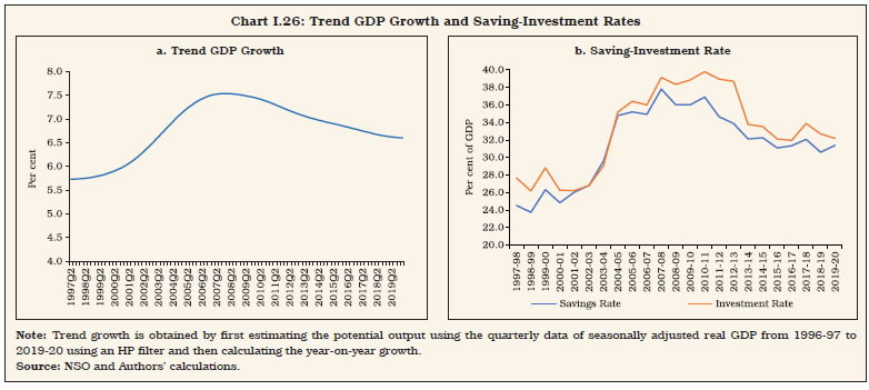
 I.56 Eventually, as policy stimuli were wound down, investment began decelerating from 2010-11, weakening the momentum of growth of the economy. In fact, the accumulation of capital stock had started retreating even earlier from its peak in 2007-08 (Chart I.28a). Given the declining pace in the growth of employment from 2004-05, the deceleration in pace of capital accumulation impacted GDP growth. In the event, it was primarily productivity growth that sustained GDP growth (Chart I.28b).
I.57 Reviving the economy over that period needed structural reforms in the factor and product markets, along with a strategy of promoting employment intensive manufacturing. In fact, India was experiencing significant improvements in labour productivity (output per unit of labour) – higher than in many advanced economies – though India’s labour force participation rate was lower relative to G-20 countries (Charts I.29a and b). I.58 Capital productivity, as measured by the incremental capital output ratio (ICOR) also fell up to 2012-13 (Chart I.30). Subsequently, improvements in the productivity of capital use could not compensate the observed slowdown in investment. I.59 In this environment, the demographic dividend started showing signs of weakening as reflected in rising life expectancy at birth and reversal in the declining age dependency ratio (Charts I.31a and b). In fact, the declining phase of the year-on-year growth in age dependency reversed from 2015, raising concerns as to whether India would be able to reap the full benefits of the demographic dividend. I.60 At the same time, the external environment also turned less favourable with various drags in operation, including rising trade protectionism, climate change compulsions and heightened geopolitical uncertainties. Consequently, India’s export performance closely mirrored global export conditions, which had been deteriorating since the GFC (Chart I.32a). India’s imports also closely related with its exports due to a large share of intermediate and capital goods (Chart I.32b). With surges of capital inflows exceeding the absorptive capacity, India became a net exporter of capital during FIT.
I.61 Thus, macroeconomic performance under FIT was marked by an increase in the volatility of growth on account of a combination of domestic and global factors (Table I.6). Appraisal of the Institutional Architecture I.62 Besides the standard assessment in terms of macroeconomic outcomes, it is worthwhile to evaluate the institutional plumbing of the FIT architecture. Failure is defined as three consecutive quarters of average headline inflation overshooting/undershooting the upper and lower tolerance levels around the target. Since the adoption of FIT, until the pre-COVID period, there was only one occasion (i.e., Q4: 2019-20) when inflation exceeded the upper tolerance level (Chart I.33)25. The breach was due to a sharp spike in food inflation (9.7 per cent in Q4:2019-20) on a combination of adverse developments, i.e., the late withdrawal of the monsoon, unseasonal rains and associated supply disruptions (RBI, 2020). 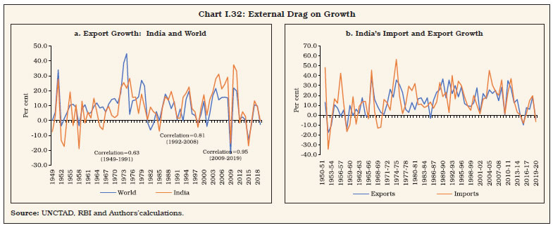
| Table I.6: Key Macroeconomic Indicators under FIT - Level and Volatility | | (Per cent) | | | Level | Volatility | | CPI-C Inflation | Real GDP Growth | Interest Rate (WACR) | App(+)/ Dep(-) of Exchange Rate (REER-36) | Combined GFD/GDP | CPI-C Inflation | Real GDP Growth | Interest Rate (WACR) | Exchange Rate (REER- 36) | Fiscal Slippage (Deviation from Centre's Budgeted GFD/GDP) | | Pre-FIT | | 2012-13 | 10.0 | 5.5 | 8.1 | -4.3 | 6.9 | 0.5 | 1.4 | 0.2 | 2.0 | -0.2 | | 2013-14 | 9.4 | 6.4 | 8.3 | -2.2 | 6.7 | 1.3 | 0.8 | 0.9 | 2.2 | -0.3 | | 2014-15 | 5.8 | 7.4 | 8.0 | 5.5 | 6.7 | 1.5 | 1.2 | 0.2 | 0.9 | 0.0 | | 2015-16 | 4.9 | 8.0 | 7.0 | 2.9 | 6.9 | 0.7 | 0.8 | 0.3 | 1.3 | 0.0 | | Average | 7.5 | 6.8 | 7.8 | 0.5 | 6.8 | 2.4 | 1.4 | 0.7 | 1.6 | -0.1 | | FIT | | 2016-17 | 4.5 | 8.3 | 6.2 | 2.2 | 6.9 | 1.0 | 1.4 | 0.2 | 0.7 | 0.0 | | 2017-18 | 3.6 | 6.8 | 5.9 | 4.5 | 5.8 | 1.2 | 1.1 | 0.1 | 1.3 | 0.3 | | 2018-19 | 3.4 | 6.5 | 6.3 | -4.8 | 5.8 | 1.1 | 0.7 | 0.2 | 1.9 | 0.1 | | 2019-20 | 4.8 | 4.0 | 5.4 | 2.4 | 6.9 | 1.8 | 0.9 | 0.4 | 1.2 | 1.3 | | Average | 4.1 | 6.4 | 6.0 | 1.1 | 6.4 | 1.4 | 1.8 | 0.4 | 1.3 | 0.4 | Note: Volatility is measured by standard deviation of monthly y-o-y inflation, quarterly y-o-y GDP, monthly WACR and monthly appreciation/ depreciation of exchange rate. Fiscal slippage is defined as the deviation of the actual GFD/GDP ratio of the central government from the budgeted levels. Average volatility indicates standard deviation of the variable for the relevant full period.
Source: Handbook of Statistics on Indian Economy, RBI; GoI Budget Documents and Authors’ calculations. | I.63 The committee approach to monetary policy decision making has been widely regarded as a means of overcoming time inconsistency by efficient pooling of information, collective wisdom and diversity of opinion that help to overcome the potential pitfalls of committee-based approaches, i.e., the dangers of groupthink and free-riding (Sibert, 2006). An analysis of the minutes of the MPC meetings reveals significant differences in the voting pattern, both on the policy rate, the stance and the individual member’s assessment of the macroeconomic situation. In the universe of 22 meetings of the first MPC (during pre-COVID period), there has been less consensus on policy rate changes than on the monetary policy stance – only on nine occasions there was a consensus on policy rate changes (6-0), while on 19 occasions there was a consensus on the policy stance (6-0). The differences on the stance were largely on the timing of change in the policy stance. The differences with the ‘majority view’ was not limited to external MPC members; even internal members had differences on the size as well as direction of policy rate changes. This is in contrast with the view in the literature that only external members help avoid “groupthink” (Sibert, 2006, op. cit). Over its tenure, the MPC took more split decisions than unanimous calls, the minutes became more detailed, and even when members agreed, their arguments and rationales often differed (Duggal, 2020). In fact, the MPC has seen it all – hikes and cuts; unanimous calls and divided views; and emergency meetings (Chapter 3 delves into these experiences and draws lessons therefrom). 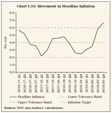 I.64 Independent assessment found that the length of monetary policy statements has dramatically declined, the linguistic complexity has improved, and the content is more focused on inflation topics since the regime change. In addition, there is a strong relationship between the length of statements and stock market volatility, highlighting the real impacts of effective communication (Mathur and Sengupta, 2020). Another interesting observation is that the discussions on inflation were dominant during the 2016-18 period, while discussions on growth have occupied more space in policy discussions from August 2019 (RBI, 2020). I.65 In order to formally analyse the MPC’s voting pattern, a Diversity Index (DI) is constructed on the basis of the voting by individual members on policy rate changes and policy stance. DI is calculated by the formula [1 - {(Number of MPC members supporting the decision minus number of MPC members opposing the decision) divided by the total size of the MPC (6 in this case)}]. The range of DI is from 0 to 1: 0 implying full agreement (6:0) and 1 implying equal division in voting (i.e., 3:3). DI also confirms large disagreement on policy rate actions, but near unanimity on the policy stance (Chart I.34). I.66 The implicit weights assigned by the MPC to inflation and output objectives can be evaluated by estimating a Taylor rule for the period from October 2016 to March 2020, i.e., taking into account all the bi-monthly monetary policy statements (Taylor, 1993). Central banks prefer to respond cautiously to a shock by changing the policy rate gradually. Therefore, an interest rate smoothing term has been included in the Taylor rule (Woodford, 2003). Thus, the estimated Taylor rule has three parameters: the weight on interest rate smoothing; the weight on the inflation gap; and the weight on the output gap. Another popular approach is to modify Taylor’s classic formulation by replacing current inflation numbers with forecasts (Taylor-type rule) (Clarida et al., 2000; Orphanides, 2003). In FIT as stated earlier, the inflation forecast becomes the intermediate target for monetary policy, representing the consolidation of the entire information set available to the MPC at the time of its decision. Considering the lags in monetary policy transmission, a three-quarter ahead inflation forecast is used for measuring the inflation gap26. 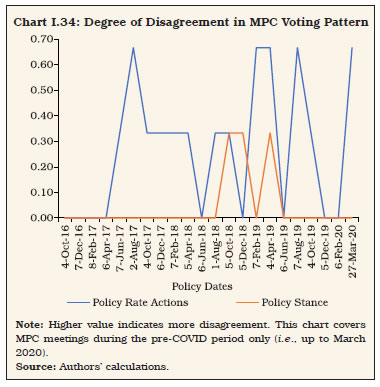 I.67 The estimated Taylor rule suggests that the MPC accorded greater importance to inflation consistent with its mandate. By and large, the approach of the MPC in aligning inflation with the target was gradualistic, reflecting its sensitivity to contingent output effects. This is reflected in the size of the smoothing parameter (Table I.7). I.68 Another estimation carried out using realised inflation (at time t) instead of the inflation forecast (at time t+3) yields an insignificant coefficient on the inflation gap, indicating that the MPC was forward-looking and not driven by past readings of inflation (at time t) while deciding the policy rate27; however, the weakening of demand conditions played a more active role in policy rate determination in the recent past (Chart I.35). Table I.7: Monetary Policy Reaction Function
(First MPC’s Tenure)# | | Smoothing Parameter | Inflation Forecast Gap (+3) | Output Gap | | 0.60*** | 0.70*** | 0.26** | *** and ** represent significance at 1 per cent and 5 per cent, respectively.
#: Covers meetings only for the pre-COVID period.
Source: Authors’ estimates. | I.69 The disagreement on policy rate decisions can also be utilised to assess individual MPC members’ contextual preferences for inflation and growth objectives. Accordingly, the Taylor rule is estimated separately for the policy rate path preferred by different MPC members as reflected in their voting patterns. The weights assigned by the MPC members on inflation and output objectives were found to be in the range of 0.63 to 0.74 and 0.24 to 0.31, respectively. The smoothing parameter also was different for different MPC members (varying in the range 0.58 to 0.68). With the same set of full information matrices available with all MPC members while casting their votes, the variation in the weighting pattern is reflective of the differences in the views and assessments of individual MPC members, indicative of individualistic behaviour rather than groupthink. 5. Conclusion I.70 To sum up, this chapter chronicles India’s formative experience with FIT in order to set up the laboratory for a review of the monetary policy framework. It provides an overview of the initial conditions that called for a change in the policy framework, followed by the setting of the pre-conditions for ushering in FIT in India and the experience with de jure FIT since 2016. In these rites of passage, existential questions emerged, each of which forms in a forward-looking manner the subject matter of dedicated chapters that follow. I.71 Chapter 2 evaluates the inflation target and the appropriateness of +/- 2 per cent tolerance band taking into account the changes in the inflation process – inflation persistence; trend inflation; food and fuel shocks; threshold level of inflation; projection errors over different time horizons; and the degree of anchoring of inflation expectations. It also evaluates the growth objective under the FIT framework. I.72 Chapter 3 drills into the monetary policy decision making process under the FIT in India, its statutory provisions, pre-policy procedures, rules and responsibilities for members individually and collectively as a Committee, communication, accountability and evaluation. The focus of the chapter is to identify what works and what needs to be fixed. I.73 Chapter 4 is about the operating framework and monetary policy transmission. It delves into the liquidity management facility and the operating target, including the reaction to announcement effects of policy changes on the operating rate. Some stylised facts of the operating procedure and transmission to various segments of the financial markets are presented. The chapter draws on this analysis to make recommendations that should help to make transmission of monetary policy impulses to its ultimate goals full, complete and timely. I.74 Chapter 5 deals with the challenges to monetary policy in an open economy framework, especially the trilemma that circumscribes its domestic orientation. Managing capital flows and exchange rate volatility are important considerations in this chapter as it looks beyond to an imminent larger role for India than before in the global economy. References Ahluwalia, M.S. (2014), “Central Banks Should not Look Only at Inflation Target”, The Economic Times, Available at https://economictimes.indiatimes.com/news/economy/policy/central-banks-shouldnot-look-only-at-inflation-target-monteksingh-ahluwalia/articleshow/28749582.cms?utm_source=contentofinterest&utm_medium=text&utm_campaign=cppst. Altissimo, F., M. Ehrmann and F. Smets (2006), “Inflation Persistence and Price-setting Behaviour in the Euro Area - A Summary of the IPN evidence”, ECB Occasional Paper, No.46. Ball, L. (1994), “What Determines the Sacrifice Ratio?.” Monetary Policy. The University of Chicago Press, 155-193,Available at https://www.nber.org/system/files/chapters/c8332/c8332.pdf Ball, L. and N. Sheridan (2005), “Does Inflation Targeting Matter?”, In: Bernanke, B. S. and Woodford, M. (Eds.), The Inflation-targeting Debate, University of Chicago Press. Bauer, A. (2018), “Lowering Inflation is a Major Structural Reform in India: IMF Official”, The Hindu BusinessLine, 2018, Available at https://www.thehindubusinessline.com/economy/lowering-inflation-is-a-major-structural-reform-in-india-imf-official/article24979922. Beck, G. W. and A. A. Weber (2005), “Price Stability, Inflation Convergence and Diversity in EMU: Does One Size Fit All?”, Centre for Financial Studies Working Paper No. 2005/30, November. Benes, J., K. Clinton, A. George, P. Gupta, J. John, O. Kamenik, D. Laxton, P. Mitra, G. Nadhanael, R. Portillo, H. Wang, and F. Zhang (2016a), “Quarterly Projection Model for India: Key Elements and Properties”, RBI Working Paper Series No. 08. Benes, M.J., K. Clinton, A. George, J. John, O. Kamenik, D. Laxton, P. Mitra, G.V. Nadhanael and H. Wang (2016b), “Inflation-Forecast Targeting for India: An Outline of the Analytical Framework”, RBI Working Paper Series No. 07. Bhoi, B. B., S. Kundu, V. Kishore, and D. Suganthi (2019), “Supply Chain Dynamics and Food Inflation in India”, RBI Monthly Bulletin, October. Bhoi, B. B., H. Shekhar and I. Padhi (2020), “Rural-Urban Inflation Dynamics in India”, RBI Monthly Bulletin, December. Clarida, R., J. Gali and M. Gertler (2000), “Monetary Policy Rules and Macroeconomic Stability: Evidence and Some Theory”, Quarterly Journal of Economics, Vol.115(1), 147-180. Duggal, I. (2020), “In Charts: The Life and Times of India’s First Monetary Policy Committee”, Bloomberg Quint, Available at https://www.bloombergquint.com/business/in-charts-the-life-and-times-of-indias-first-monetary-policy committee. Eichengreen. B., P. Gupta and R. Choudhary (2020), “Inflation Targeting in India: An Interim Assessment”, NCAER India Policy Forum, July. Engle, R. F., and C. W. Granger (1987), “Co-integration and Error Correction: Representation, Estimation, and Testing”, Econometrica, Vol.55(2). Fraga, A., I. Goldfajn and A. Minella (2003), “Inflation Targeting in Emerging Market Economies”, NBER Macroeconomics Annual 2003, Vol. 18, 365-400. Fuhrer, J. C. (2010), “Inflation Persistence”, In Handbook of Monetary Economics, Vol.3, 423-486. Gokarn, S. (2010), “Monetary Policy Considerations after the Crisis: Practitioners’ Perspectives”, Plenary Lecture at the Conference on Economic Policies for Inclusive Development, Ministry of Finance, Government of India and National Institute of Public Finance and Policy at New Delhi. Goncalves, C. E. S. and J. M. Salles (2008), “Inflation Targeting in Emerging Economies: What do the Data Say?”, Journal of Development Economics, Vol.85, 312–318. International Monetary Fund (2011), World Economic Outlook, September. Jahan, S. (2017), “Inflation Targeting: Holding the Line”, IMF Finance and Development, November. Jalan, B. (2017). “Inflation Targeting’ Can’t Work in India: Former RBI governor Bimal Jalan”, The Economic Times, Available at https://economictimes.indiatimes.com/news/economy/indicators/inflation-targeting-cant-work-in-india-former-rbi-governor-bimal-jalan/articleshow/59341674.cms?from=mdr. Kundu, S., V. Kishore and B. B. Bhoi (2018), “Regional Inflation Dynamics in India”, RBI Monthly Bulletin, November. Mathur, A. and R. Sengupta (2020), “Analysing monetary policy statements of the Reserve Bank of India”, IGIDR Working Paper WP-2019-012, April. Mishkin, F. S. and K. Schmidt-Hebbel (2007), “Does Inflation Targeting make a Difference”, NBER Working Paper 12876, January. Mohan, R. (2011), Growth with Financial Stability. Oxford University Press. New Delhi. Orphanides, A. (2003), “Historical Monetary Policy Analysis and the Taylor Rule”, Journal of Monetary Economics, Vol.50(5), 983-1022. Patra, M. D., J. K. Khundrakpam and A. T. George (2014), “Post-Global Crisis Inflation Dynamics in India: What has Changed?”, In NBER India Policy Forum, 2013–14, Vol.10(1), 117-203. Patra, M. D. (2017), “One Year in the Life of India’s Monetary Policy Committee”, Remakes at the Regional Office of the Reserve Bank of India, Jaipur, 27 October 2017, Published as Bank of International Settlements Central Bankers’ Speeches, Available at https://www.bis.org/review/r171123e.pdf. Pesaran, M. H., Y. Shin and R. J. Smith (2001), “Bounds Testing Approaches to the Analysis of Level Relationships”, Journal of Applied Econometrics, Vol.16(3), 289-326. Phillips, P. C. B. and B. E. Hansen (1990), “Estimation and Inference in Models of Cointegration: A Simulation Study”, Advances in Econometrics, Vol. 8, 225-248. Reserve Bank of India (2010), Annual Report, 2009-10. Reserve Bank of India (2012), Annual Report, 2011-12. Reserve Bank of India (2014), Annual Report, 2013-14. Reserve Bank of India (2020), Annual Report, 2019-20. Reddy, Y. V. (2005), “Monetary Policy: An Outline”, RBI Monthly Bulletin, March. Reddy, Y.V. (2008), “The Virtues and Vices of Talking About Monetary Policy – Some Comments”, Remarks at the 7th BIS Annual Conference, Luzern, Switzerland. Shaw, P. (2019), “Using Rational Expectations to Predict Inflation”, RBI Occasional Papers, Vol. 40(1). Sibert, A. (2006), “Central Banking by Committee.” International Finance, 145-168. Subbarao, D. (2016), Who Moved My Interest Rate?: Leading the Reserve Bank of India Through Five Turbulent Years, Penguin Random House India Private Limited. Taylor, J. B. (1993), “Discretion versus Policy Rules in Practice”, In Carnegie-Rochester Conference Series on Public Policy, Vol.39, 195-214, North-Holland. Verick, S. and I. Islam (2010), “The Great Recession of 2008-2009: Causes, Consequences and Policy Responses”, The Institute for the Study of Labor (IZA) Discussion Papers No. 4934, May. Weyerstrass, K., B. Aarle, M. Kappler and A. Seymen (2011), “Business Cycle Synchronisation within the Euro Area: In Search of a ‘Euro Effect’”, Open Economies Review, 22(3), 427–446. Woodford, M. (2003), “Optimal Interest-rate Smoothing”, The Review of Economic Studies, Vol.70(4), 861-886.
|