Press Release
RBI Working Paper Series No. 02 Regional Economic Convergence in the Manufacturing Sector:
An Empirical Reflection Madhuresh Kumar@ Abstract 1 This paper uses data on registered manufacturing from the Annual Survey of Industries (ASI) for the post global financial crisis period (2008-09 to 2017-18) and examines the convergence pattern of 21 major states in India and their key drivers. While poorer states are found to have exhibited convergence to the mean Net Value Added per capita (NVApc), richer and middle-income states displayed divergence. Poorer states registered the fastest rate of growth among the three groups, driven by the highest rate of growth in fixed capital. They experienced the lowest rate of growth in labour and the contribution of total factor productivity growth (TFPG) was also negative, suggesting the role of high capital intensity in driving convergence. Richer states exhibited highest rate of growth in labour and the contribution of TFPG was also positive, which enabled them to perform better on overall growth compared with the states in the middle-income category. Within each group, this paper finds evidence of convergence to the mean NVApc. JEL classification: O14, O16, O47, O53 Keywords: Convergence, productivity, capital intensity, GMM. Introduction A strand in the growth literature emphasises the importance of regional convergence and their drivers to understand the overall growth dynamics in the economy. The Neoclassical growth theory (NCGT) presumes that the poorer economies should converge to their richer counterparts benefitting from higher marginal productivity of capital. The empirical findings, however do not show any systematic propensity for convergence and at best what one can find is conditional convergence, i.e., after controlling for various economy specific variables. In the case of states or regions within a country, researchers have found some evidence of regional convergence (Barro and Sala-i-Martin, 1992; Sala-i-Martin, 1996) in the richer Organisation for Economic Co-operation and Development (OECD) countries, but the evidence in the case of developing economies has been mixed (Isabela, 2006; Hoshino, 2012, etc.). Rodrik (2013) has argued that unconditional convergence occurs, but in the modern parts of the economy (e.g., registered manufacturing2 and tradable services) rather than the economy as a whole. The convergence in manufacturing activities may not lead to overall convergence because of the following facts: (1) non-manufacturing activities do not exhibit unconditional convergence; (2) poor countries have little employment in manufacturing, depressing the contribution of manufacturing to overall growth; (3) the share of employment in manufacturing rises over the course of development, giving less-poor countries a growth boost; and (4) the reallocation effect is neither sizeable nor systematically larger at lower income levels. In terms of magnitude of impact, the first two factors play dominant roles. From the standpoint of an economy, however, the last assertion is perhaps most interesting, pointing to an important unexploited potential in poor countries. The convergence literature in the Indian context has not delved into the manufacturing activities and has mostly focused on the gross state domestic product (GSDP) per capita. Empirical evidence on convergence of the Indian states has been mixed. Furthermore, most of the studies are limited to analysing the trend of convergence/ divergence but have not made adequate effort to explain the sources of the apparent trend. Our study tries to fill this gap in the literature. India’s organised manufacturing sector rebounded impressively after slowing down during 2007-09 at the height of the global economic crisis. But that revival has been short-lived, reflecting sluggish employment and output growth conditions. Have these conditions impacted the regional economic convergence/divergence in the registered manufacturing sector? Additionally, a comprehensive review of the foreign direct investment (FDI) policy was undertaken in 2007-08 and a more liberal FDI regime is expected to funnel more investments in the industrially developed states as the top five states along with Delhi NCR receive the major chunk of the total FDI inflows. Nonetheless, analysis of FDI data has shown that after the boom period of 2004-05 to 2008-09, the growth rate of FDI inflows tapered off subsequently. To put it in perspective the nominal yearly growth rate of FDI during 2000-01 to 2008-09 was 34 per cent which moderated to 4.3 per cent in the 2008-09 to 2017-18 period. This slowdown in FDI inflows is expected to affect the more industrialised states since they are the major beneficiaries of the FDI inflows. The study seeks to analyse the Indian growth story of registered manufacturing3 in the post-Global Financial Crisis period. Using ASI data (registered manufacturing) for the period of 2008-09 to 2017-18, the major Indian states are classified, on the basis of initial manufacturing NVApc, into three groups, viz., Group A4 (rich) states are those whose NVApc is one standard deviation above of the mean NVApc, while Group B5 (middle-income) states comprise of states having NVApc between one standard deviation above and below of the mean NVApc. The rest of the states are classified as Group C6 (poorer) states7. The paper attempts to address the following questions: a) Whether the above-mentioned three groups are converging or diverging to the mean NVApc. Are states within a particular group converging towards the group’s mean (club convergence)? b) Whether the major Indian states have converged or diverged during the sample period? c) What explains the observed divergent/convergent patterns? The rest of the paper is organised as follows: Section II reviews the literature on convergence/ divergence, while section III covers methodology and data. Empirical findings are discussed in section IV. Section V concludes the study. II. The Literature There is a sizeable literature on regional disparity in India, with studies using different indicators, time periods and methodologies. A common perspective of this literature is that most of the studies provide evidence of divergence rather than convergence. Illustratively, Nair (1971) does not find any tendency of convergence of income levels for the period 1950-1960. About three decades later, Cashin and Sahay (1996) examined the growth experience of 20 major states of India during 1961-91. Using the analytical framework of the Solow-Swan neoclassical growth model and cross-section estimation, they found evidence of absolute convergence, but the dispersion of real per capita income widened during the period. However, Cashin and Sahay (1996) was contested by Govinda Rao and Kunal Sen in IMF staff paper (1997) on conceptual and methodological issues (e.g., absolute convergence holds only when manufacturing variable is included to control for sectoral shocks but Rao et al. find the inclusion of this variable as irrelevant). Similarly, Rao, Shand and Kalirajan (1999) suggested that the per capita State Domestic Product (SDP) diverged and the growth rate of per capita SDP positively related to states’ initial income levels. Ahluwalia (2000) used the Gini coefficient to show divergence among the states during 1980-97. Sachs, Bajpai, and Ramiah (2002) studied the growth experiences of 14 major states of India during 1980-1998 by using sigma (σ)-convergence and beta (β)-convergence measures to examine whether per capita income in the states have been converging or diverging. By both standards of convergence, India demonstrated overall divergence during 1980-98, as well as during both the pre-reform and post-reform sub-periods. Also, they found that the richer states experienced a degree of convergence during the post-reform period, while the poorer states did not. Divergence was most notable within the poorer group of states. Adabar (2004), while investigating the 14 major states in the study period of 1976-77 to 2000-01 found absolute divergence. However, after controlling for per capita investment, population growth rate and human capital along with state-specific effects, they found the evidence of conditional convergence at around 12 per cent per five-year span. Bhattacharya and Sakthivel (2004) found that during both the pre-reform and post-reform periods, the divergence occurred, but the divergence was much more rapid in the post-reform period. Bandyopadhyay (2006) examined the period 1965-97 and concluded that the disparities across the states declined in the 1960s and then increased thereafter. He found two income convergence clubs at 125 per cent and 50 per cent of the national income average. Das et al. (2010) found convergence in per capita consumption (during 1958-2005) only in urban areas, while the rural areas diverged. Chitke (2011) studied 15 states and found a strong evidence of divergence in per capita income of the states during the sample period of 1970-2005. The standard deviation of the net state domestic product increased over time indicating no evidence of convergence in the pre- or post-reform period. Population, state capital expenditure and commercial bank credit have also diverged over time across these 15 Indian states. However, literacy rate showed evidence of convergence across states. Das et al. (2013) have found evidence of conditional convergence among the states. Tirtha Chatterjee (2014) has found β convergence but not σ convergence while analysing per capita income convergence in Indian agriculture across the states. Mishra and Mishra (2015), while examining income convergence for 17 major states of India for the period of 1960-2012, find evidence for convergence with two structural breaks in the series. Pandya and Maind (2017) also find strong evidence of β convergence using dynamic panel data model for the period 1990-2011. Chanda and Kabiraj (2018) have found overwhelming evidence of absolute convergence using night-lights data. Roy, Sen and Sanyal (2019) find no discernible evidence of convergence across the states, especially post-liberalization. However, taking into account control variables for capital expenditure, development expenditure, and fiscal deficit, they find significant evidence of convergence of state-level per capita GDP. In the international context, convergence hypothesis has been empirically tested by Barro and Sala-i-Martin (1992), analysing 73 European regions (since 1950) and 48 states of the USA (since 1880). The study found the existence of conditional convergence in the European region and unconditional convergence among the states of the USA. In further research, Sala-i-Martin (1996) included Japanese prefectures and Canadian provinces and concluded that regions tend to converge at a speed of approximately 2 per cent per year, which resulted in diminishing interregional dispersion of income over time. However, Tsionas (2000) found no convergence in the USA over the sample period (1977-1996). Young et al. (2008) find β convergence among the US states, but at the same time, they also find σ divergence. Maria Isabel Serra et al. (2006) found very weak to nil unconditional convergence evidence in select Latin American countries from 1970 to 2000. China has also experienced divergence post the reforms of 1978. Masashi Hoshino (2012) in his study has found regional divergence in Russia, India and China. The literature thus shows that most of the studies focused on the convergence/ divergence of the overall per capita income. However, Rodrik (2013) has departed from this tradition and has persuasively shown that unconditional convergence has occurred in the organised manufacturing in the sample of more than 100 countries. Françoise Lemoine et al. (2014) have investigated whether the Chinese provinces are converging in industrial output and have found rapid and unconditional convergence in the Chinese manufacturing industry from the 1990s to mid-2000s. This study too departs from the traditional focus on GDP per capita and focuses on registered manufacturing activities to provide an alternative perspective. The study considers gross value added per capita in registered manufacturing sector as the benchmark to ascertain whether the states are converging or diverging. More importantly, it tries to ascertain the reasons underlying the divergence/convergence phenomenon. III. Methodology and Data The theoretical foundation for the methodology adopted in this study is derived from the neoclassical growth model. According to this framework, convergence in terms of both growth rate and income level requires what is called β convergence. This follows from the assumption of diminishing returns, which implies higher (lower) marginal productivity of capital in a capital-poor (rich) economy. With similar savings rates, poorer economies, therefore, grow faster. If this scenario holds, there should be a negative correlation between the initial income level and the subsequent growth rate. This led to the popular methodology of investigating convergence, i.e., the growth-initial level income regression. The coefficient of the initial income variable in this regression model is supposed to pick up the negative correlation (Islam, 2003). For elucidation of the methodology, let us consider the neoclassical growth theory, according to which economies tend to converge to their steady state income level: 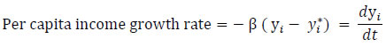 where yi* is the steady state per capita income, yi is the present per capita income. After manipulation, it can be expressed as: where subscripts i and t denote state and time, T is the length of time, and y is NVApc of registered manufacturing taken from ASI data. The dependent variable ‘growth’ is explained by the independent variable ‘initial NVApc’. If the steady state y*i and the speed of technological progress xi were the same in all the economies, then the term ai = a and, when the coefficient β is negative, the poorer economies would outgrow the richer ones (Kangasharju, 1998). The value of coefficient λ could be calculated from the above set of equations which gives the speed of convergence. The above cross-sectional regression assumes that the states converge towards a unique steady state income where all the elements that affect steady state income is assumed to be similar across all the economies (unconditional or absolute convergence). Nevertheless, if the heterogeneity in the parameters are allowed for, then the economies reach different steady state incomes. The assumption that economic-specific, time-invariant fixed effects exist, which are responsible for individual steady state income positions (Rodriguez, 2008). The above cross-sectional regression analysis does not allow to estimate the individual state-specific effects to the full extent because of its assumption of identical steady state income of all the economies. Individual states may approach their own steady state income based on their underlying idiosyncratic parameters. To overcome the limitations of cross-sectional regression, a panel data approach has been adopted. However, it may be noted that the concept of convergence in panel data framework differs from that of cross-sectional approach in the sense that it is now regarded as convergence towards the region´s own steady state income rather than a unique steady state income which is assumed to be the same for all the economies irrespective of their underlying parameters. Equation (1) has been reformulated into a panel data model (as is done by Islam (1995) in Growth Empirics – A Panel data Approach);  where, yit = NVA per capita, xit = ln (s/n+g+δ), η = time dummy, µi = unobserved state specific effect, νit = error term, s = (Gross fixed capital formation/GVA), n = growth rate of total persons engaged, g = exogenous rate of technological progress and δ = depreciation rate of fixed capital. Following Mankiw, Romer and Weil (1992), (g+δ) has been assumed to be 0.05. The presence of an autoregressive term in the equation makes the use of the Least Square Dummy Variables (LSDV) estimator redundant because the lagged dependent variable will always be related to the error term. This is due to the fact that both dependent and lagged dependent variables are a function of µi. As a result, yi,t-1 is correlated with the error term (B N Rath and Madheswaran, 2010). There are several approaches to overcome this problem. However, in this paper, the panel model is estimated using the Arellano-Bover/Blundell-Bond Generalized method of moments (GMM) estimator, which is an extension of the Arellano-Bond model, where past values and different transformations of past values of the potentially problematic independent variable are used as instruments together with other instrument variables. The Arellano–Bover/Blundell–Bond estimator augments Arellano–Bond by making an additional assumption that first differences of instrument variables are uncorrelated with the fixed effects. This allows the introduction of more instruments and can dramatically improve efficiency. It builds a system of two equations—the original equation and the transformed one—and is also known as system GMM (Engblom, 2015). The single cross section is modified into a panel framework by dividing the total period into several shorter time spans. The next logical question that arises is what the appropriate length of such time spans would be. According to Islam (1995), technically one can go up to one-year time span, given that the underlying data set provides annual data. However, for several reasons, it seems that the yearly time span is too short to be appropriate for studying convergence. Short-term error terms may appear large in such brief time spans. In this study, we opt for three-year time intervals. An alternative to the above approach, popularly known as σ convergence, derives from the seminal works of Quah (1993a) and Friedman (1994) and several other studies inspired by them. According to this school of thought, convergence is a proposition regarding the dispersion of the cross-sectional distribution of income, and a negative coefficient from the growth-initial income level regression does not necessarily imply a reduction in this dispersion. Thus, instead of judging indirectly and perhaps erroneously through the sign of β, convergence should be judged directly by looking at the dynamics of dispersion of income level across the economies. This gave rise to the concept of σ convergence, where σ is the notation for standard deviation of the cross-sectional distribution of either income level or growth rate (Islam, 2003). Following is the relationship between β and σ convergence and it will show why β convergence, although a necessary condition, doesn’t necessarily imply σ convergence. The income of the ith economy can be approximated by the following equation: The equation (2) can be used to derive the evolution of σ2t, variance of yit, and is described by: Only if -1<β<0, the difference equation is stable8, therefore β convergence is a necessary condition for σ convergence. Given -1<β<0, the steady state variance is Thus, the cross-sectional dispersion falls with β becoming more negative but rises with σ2u. Combining equations (3) and (4) we get, which is a first-order linear difference equation with constant coefficients. Its solution is given by where, c is an arbitrary constant. Thus, as long as -1 <β<0, we have |1 + β| < 1, which implies that as t → ∞ Moreover, as (1 + β) > 0, the approach to (σ2)* is monotonic and σ2t can either increase or decrease monotonically towards (σ2)* (Young et al., 2008). Therefore, even with β convergence, the dispersion of per capita income can keep on increasing as has been observed empirically in many studies. The σ convergence occurs when the dispersion of real per capita income across the regions fall with time. For the empirical approach here, the coefficient of variation (CV) is calculated for the whole sample of 21 states and also for the groups of states, with CV defined as where, CV = coefficient of variation, Ῡ = mean NVA per capita income, and σ2 = variance of NVA per capita income. However, while handling with log transformed data, the CV is given by: Convergence/divergence is the manifestation of another underlying process, which is differential rate of growth. The main sources of the long-term growth are technological advancement, capital accumulation and increase in labour inputs. In accounting for the sources of growth, a simple production function having constant returns to scale of the following form (where capital and labour are the only factor inputs) is considered; where A is termed as the total factor productivity while α and β are the share of capital and labour, respectively, in the gross value added (GVA). Sum of the share of capital and labour is 1. Then growth in Y (GVA) is  Thus, the growth in GVA can be decomposed into total factor productivity growth9 and the growth from capital and labour inputs. Labour (total number of persons engaged) growth, capital (real fixed capital) growth and NVA growth are computed using ASI data. For estimating the total factor productivity growth (TFPG), the growth accounting (GA) method, which is widely used in India for estimating TFPG of the manufacturing sector has been considered. This approach measures TFPG as the difference between the rate of growth of output and the weighted rates of growth of factor inputs. In this paper, the Divisia-Tornquist (D-T) approximation has been used for the calculation of TFPG (Balakrishnan et al., 1994). The TFPG under the D-T approximation is given by the following equation:  where Q denotes Gross Value Added, Xi factors of production and si shares of factors of production (assumed that there are only two factors of production, viz., labour and capital). In the growth accounting framework, information about the share of each factors of production (si) in the value added is required. The share of emoluments in gross value added is considered as the share of labour. Assuming constant returns to scale, the share of capital is one minus the share of labour (Kathuria et al., 2014). Here, value added single deflation method is used, i.e., Gross value added is deflated by WPI manufactured products. The measurement of capital stock has been a very contentious issue. Fixed capital can be obtained from the ASI data set, but the net fixed asset given in the ASI is at book value and not at replacement cost, and hence, we cannot use it for TFPG calculation. Depreciation series is also given in the ASI data but it also suffers from the same problem. To overcome this difficulty, perpetual inventory accumulation method (PIAM) has been used to generate a series on capital stock. The series on book value of fixed capital and depreciation to construct gross fixed capital formation series have been used. For this, first, we need to estimate capital stock in the benchmark year and investment in the subsequent years. The nominal gross fixed capital formation (I) figures are calculated as follows: where BV denotes the book value of fixed capital (as given in the ASI data), D denotes depreciation. The capital stock (K) in any year can then be calculated as follows: To get reliable results, we need long series on capital stock data. For this purpose, 1981-82 has been taken as the benchmark year which gives a fairly long series on capital stock. K0 denotes the capital stock in 1981-82. The capital stock series have been calculated at 2008-09 prices by using the Investment Deflator Series. This series was obtained by using the data on gross fixed capital formation at current and constant price. The depreciation of fixed capital is taken at 5 per cent per annum. Empirically, across many countries and over time periods, a positive correlation between TFPG and capital intensity has been found. The hypothesis is that there are positive interactions between capital accumulation and technological advances. There are several avenues through which capital formation and total factor productivity growth may be associated. First, it is likely that substantial capital accumulation is necessary to put new inventions into practice and to affect their widespread employment. This association is often referred to as the ‘embodiment effect’, since it implies that at least some technological innovation is embodied in capital. It is also consistent with the ‘vintage effect’, which states that new capital is more productive than old capital per (constant) dollar of expenditure. A second avenue is that the introduction of new capital may lead to better organisation, management, and the like. This may be true even if no new technology is incorporated in the capital equipment. A third avenue is through learning-by-doing. Thus, technological progress should be correlated with the accumulation of capital stock. Fourth, potential technological advance may stimulate capital formation, because the opportunity to modernise equipment promises a high rate of return on investment. A fifth avenue is through the so-called Verdoorn (1949) or Kaldor (1967) effect, whereby investment growth may lead to a growth in demand and thereby to the maintenance of a generally favourable economic climate for investment. Such positive feedbacks may act cumulatively (Edward Wolff, 1991). Thus, a higher growth in capital intensity should normally be correlated with higher productivity growth. Whether this relationship holds in the Indian scenario has been examined in the study. In this study, capital intensity is computed as the ratio of real fixed capital to the total persons engaged. The fixed capital as defined in ASI document represents the depreciated value of fixed assets owned by the factory as on the closing day of the accounting year. Fixed assets are those that have a normal productive life of more than one year. Fixed capital includes land including leasehold land, buildings, plant and machinery, furniture and fixtures, transport equipment, water system and roadways and other fixed assets such as hospitals, schools, etc. used for the benefit of the factory personnel. Total persons engaged include the employees and all working proprietors and their family members who are actively engaged in the work of the factory even without any pay, and the unpaid members of the co-operative societies who worked in or for the factory in any direct and productive capacity. The number of workers or employees is an average number obtained by dividing mandays worked by the number of days the factory had worked during the reference year (ASI). IV. Empirical Findings On the first research question as to whether the groups of states are converging or diverging, the barometer for the groups to converge is the closing of Gap10 between their share of NVA and share of population. Table (1) provides some stylised facts about registered manufacturing sector for the sample of states studied in this paper. In 2008-09, the share of NVA of the middle-income states was pretty close to their population share. The skewness in the distribution of income could largely be attributed to the disproportionately large (small) share of NVA of the rich (poor) states. The richer and the poorer states increased their share in NVA by the end of 2017-18 at the cost of the middle-income states. The reason for the middle- income states yielding their share to the other groups was their below average growth performance at around 4 per cent of compound annual growth rate (CAGR), while the rich and poor states grew at above average rates, thereby gaining in the share of NVA. Group C states, by clocking the highest growth rate (7.24 per cent), managed to close the Gap, whereas the Gap for the other groups increased. Rich states increased the Gap by increasing their share of NVA while the middle-income states did so by reducing it. Thus, only the poorer states evinced convergence while the other groups diverged from the average NVApc11. Although, the share of population of the rich states only being 29 per cent, it employed 54.4 per cent of the labour force in 2008-09 which further increased to 57.5 per cent by the end of 2017-18. On the other hand, despite having 47 per cent of the population, the poor states only employed 21 per cent of the labour force which further reduced to 19.47 per cent by 2017-18. The employment share of the middle-income states also shrank in this period; however, the difference between its population and employment share is not that conspicuous. | Table 1: Manufacturing Sector-Stylised Facts (in per cent) | | | Group A | Group B | Group C | | Share of NVA (2017-18) | 63.56
(+ 2.44) | 15.25
(-3.52) | 17.52
(+1.16) | | Share of NVA (2008-09) | 61.12 | 18.77 | 16.36 | | Share of employment (2017-18) | 57.50
(+ 3.10) | 19.90
(-1.11) | 19.47
(-1.54) | | Share of employment (2008-09) | 54.40 | 21.01 | 21.01 | | Share of population (2011 Census) | 29 | 21 | 47 | | Growth of real NVA | 6.89 | 3.99 | 7.24 | | Overall growth of NVA (of 21 major states) | 6.43 | Note: Figures in parenthesis show percentage change.
Source: Authors’ calculation from ASI data. | The group divergence/convergence notwithstanding, a pertinent issue here is whether the whole sample of 21 states could show divergence or convergence with respect to all-India level mean growth. Secondly, whether the same tendencies are exhibited among the particular groups as well. The empirical findings in the next section throw light on these aspects. The Convergence Evidence Table 2 presents the results of our estimation using the cross sectional (unconditional convergence) regression. The implied convergence speed (λ) from cross sectional regression comes out to be approximately 0.7 per cent per annum. The results indicate that there was indeed unconditional convergence during the study period 2008-09 to 2017-18. It may be noted that the above derivation in λ and of equation (1) is entirely on the basis of growth process within an economy, and there is no reference to what is happening across economies. This shows that λ essentially refers to a within-economy process and denotes how fast an economy is closing the gap between its own current and the steady state income. Therefore, ‘λ’ cannot be interpreted as the rate at which the poor economies are closing their income gap with the richer economies. However, in equation (1), we are estimating unconditional convergence in which the steady state income of presently rich and poorer states are the same, thus making the across and with-in interpretation of ‘λ’ valid. Therefore, in this case, with the assumption that all the states are approaching the same steady state income, the convergence rate of 0.7 per cent may be interpreted as the rate at which the poorer states are catching up with the richer ones12. With this rate of convergence, it will take around 98 years to reduce the income inequalities between the states by fifty per cent. In other words, the half-life being 98 years. The assumption of identical steady states masks significant heterogeneities among the states. The panel data framework enables us to account for the unobserved state-specific component (also implying that the different economies reach different steady states). Table 3 presents the results of our estimation using system GMM. The implied ‘λ’ comes out to be 8.7 per cent (half-life being around 8 years), which is considerably higher than that obtained from cross-sectional regression. This was expected, as the concept of convergence in a panel data regression is somewhat different than the classical approach of convergence in cross-section regressions. Here, λ is regarded as convergence towards the economy’s own steady state as opposed to the average steady state of the group (as in the unconditional cross-sectional analysis). | Table 2: Single Cross Section Results (21 States) (2008-09 to 2017-18) | | Dependent Variable: Growth | | Explanatory Variables | | | Initial income | -0.058 (0.068) | | Constant | 1.014 (0.581) | | Implied λ (speed of convergence) | 0.7 per cent | | R2 | 0.364 | | Note: Figure in parentheses are standard errors. |
| Table 3: Results of Estimation of System GMM Model | | Dynamic Panel data model; Dependent Variable (Initial Income) | | Explanatory Variables | | | Ln (y i, t-1) | .767 (.077) | | Ln (x i,t) | -.0232 (.0719) | | Constant | 2.214 (.7088) | | Implied λ (speed of convergence) | 8.7 per cent | | Note: Figure in parentheses are robust standard errors. | Thus, the measure of β convergence shows that the major Indian states have actually converged in terms of per capita income of the registered manufacturing sector measured by ASI data. As a measure of σ convergence, the coefficient of variation (CV) of log real NVA per capita has decreased for Indian states in the study period. As shown in Chart 1(a), the dispersion of income of Indian states has reduced implying convergence, though the magnitude of convergence is quite low. Both β and σ convergence estimates point to the convergence of the Indian states. The study also tries to investigate whether there is any evidence of ‘club convergence’13? β convergence test was not carried out in this case as the number of states in a particular group were too small to carry out any such analysis. However, the CV of NVApc of all the three groups has come down and the sigma convergence test shows that the groups too exhibited the tendency to converge (Chart 1 (b, c, d)). It may be noted that the highest percentage change of CV was for Group B states at 29 per cent followed by Group A states at 8.7 per cent. While for overall India, the σ convergence was not that strong (only 1.9 per cent). Same was the story for Group C states as the percentage change of CV was only 1.8 per cent. The TFPG of the Indian registered manufacturing during 2008-09 to 2017-18 shown in Table (4) below: | Table 4: Total Factor Productivity (TFP) Index | | | 2008-09 | 2017-18 | | GR A states | 100.0 | 109.2 | | GR B states | 100.0 | 82.1 | | GR C states | 100.0 | 88.9 | | India | 100.0 | 100.3 | | Source: Author’s calculation. | As capital stock for 1981-82 has been taken at the book value, it can induce errors in TFP calculation. Therefore, to check the robustness of the result, the initial capital stock levels were changed, first increasing it by 20 per cent and then decreasing it by 20 per cent. In both cases, there was no significant change in the results. The productivity growth in registered manufacturing sector has stagnated in the study period (the index remained almost flat). The worst performers in terms of productivity growth were the middle-income states, followed by the poorer states. However, the rich states have become more productive. The poorest states grew faster than other groups in line with the neo-classical growth theory, but did this growth occur through the same channel as predicted by the theory? To get a clearer picture of what happened at the sub-national level, the growth has been decomposed into its constituents, viz., growth in factor inputs and TFPG. Since it is assumed that capital and labour are the only two factor inputs in the production, growth has been broken down into capital, labour and TFP growth. | Table 5: Sources of Growth (2008-09 to 2017-18) | | Average Growth Per Annum (%) | Group A | Group B | Group C | India | | Capital growth | 6.5 | 8.3 | 10.7 | 7.7 | | Labour growth | 4.3 | 3.0 | 2.8 | 4.1 | | TFP growth | 0.98 | -2.17 | -1.30 | 0.02 | | GVA growth | 7.2 | 5.1 | 8.0 | 6.9 | | Source: Author’s calculation. | As is evident from Table (5), the growth in Group A states is primarily driven by the growth in labour and total factor productivity. In terms of capital growth, it lags behind both the groups. While Group C states were propelled to the top of the growth chart mainly by their high growth of capital. It did a poor job on the employment generation front and clocked a mere 2.76 per cent of CAGR, which was lowest among the groups. The TFP also declined in this category. Thus, the catch-up effect exhibited by the poorer states was not through the productivity channel but through extensive use of capital. For the Group B states, the growth in both capital and labour was moderate but the productivity decline was the highest. The trends in capital intensity in the various groups provide interesting insights. Chart 2 shows D(K/L) for the various groups of states. Here, D(K/L) is defined as the difference between Ln(K/L) of that particular group with that of India’s mean Ln(K/L). A positive value of D(K/L) shows that the capital intensity of that particular group was higher than the mean of all India. 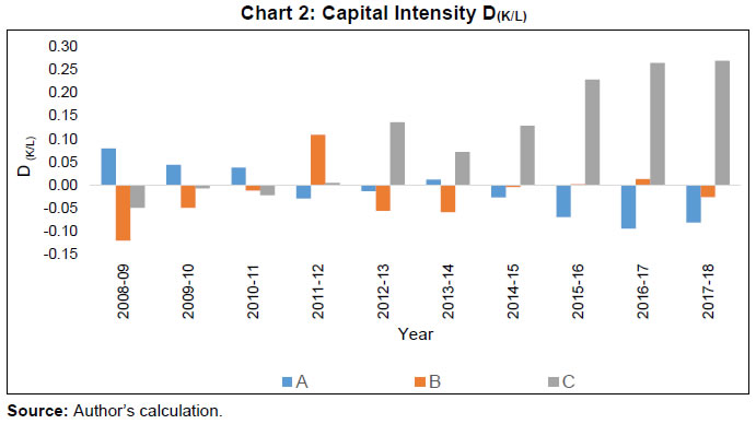 The change in the capital intensity of Group A states in relation to the other groups is interesting to note. Beginning with the most capital-intensive group in 2008-09, it became the least capital intensive by 2017-18 with a CAGR of capital being only 6.8 per cent. The Group C states’ impressive growth in capital intensity was the result of the double-digit capital growth (10.7 per cent CAGR) in this period. The next question that arises is whether this reversal in capital intensity is the result of Group A states investing less or the Group C states investing more? The long-time average of the fixed capital growth in registered manufacturing (as per ASI data) has been around 6.5-7.5 per cent (PIAM method) and the Group A were investing around this rate in the study period. It was the Group C states which have really picked up investment and not only caught up in the capital intensity but actually surpassed the Group A states. Also, the labour growth in Group A states was higher than the other groups, which further dragged its capital intensity. The growth of capital formation was highest in Bihar followed by Odisha and Madhya Pradesh. The impressive growth rate of capital in Odisha on an already high base was the major contributor in pulling up the capital intensity of the entire group (the highest growth observed by Bihar was on a low base). Sans Odisha, this anomaly, of the poorer states having the highest capital intensity disappears. Nevertheless, the growth of capital formation of the poorer states was highest even after discounting Odisha. As mentioned earlier, empirically, across many economies and time periods, a positive correlation between TFPG and capital intensity has been found and especially in an economy which starts with lower capital intensity. But in this case, the group which saw the least relative growth in capital intensity actually improved its productivity, while the Group C states became less productive. V. Concluding Observations This paper uses ASI data for 2008-09 to 2017-18 and divides 21 major states into three groups based on their initial NVApc to examine convergence. It finds that the Group C (poorer) states converged to the average NVApc, while the other two diverged. The rich states (Group A) diverged by increasing their share in NVA and the middle-income states by ceding their share in NVA. Nevertheless, at the all-India level, the sample of 21 major states exhibited both σ and β convergence. The unconditional cross-sectional β convergence results show that the states are converging approximately at the rate of 0.7 per cent per annum. While in the panel data framework, the convergence rate was at 8.7 per cent per annum14. The convergence rate is much higher in the panel data framework than in the cross-sectional one. When a panel data regression of convergence is performed the concept of convergence is somewhat different to the classical approach of convergence in cross-section regressions in the sense that it is now regarded as convergence towards the region´s own steady state income. Consequently, as a region is closer to its own steady state than to the average steady state of a total group, the convergence coefficient is higher than in the cross-section analysis (Rodriguez, 2008). Within the groups as well, the dispersion of their income has decreased signifying the occurrence of club convergence. The next issue examined in this paper is what explains the divergent (rich and middle-income states)/convergent (poor states) patterns in this context? The growth rate of poorer income states was found to be the highest among the groups, buoyed by the high growth of capital. The double-digit growth in capital formation overshadowed the relatively weaker rise in labour growth and productivity decline. On the contrary, the rich states owe their growth to labour and productivity growth. Their capital growth was the least as compared to the other groups. The middle-income states lost out primarily due to the productivity decline, even though their labour and capital growth was moderate. An interesting finding of this study is that the poorer and middle-income states are now using more capital-intensive techniques of production than the richer states. Additionally, the rising capital intensity was negatively correlated with productivity, which runs contrary to the widespread empirical evidence. Also, the source of growth for the poorer states is a concern, as their growth is driven by intensive use of capital, not by labour or productivity enhancement. Mere increases in inputs, without an increase in the efficiency with which those inputs are used - investing in more machinery - must run into diminishing returns; input-driven growth is inevitably limited (Krugman, 1994). Furthermore, this growth is not fueled by labour, which the poorer states are more abundantly endowed with.
References Abramovitz, M. (1956). Resource and Output Trends in the United States since 1870, American Economic Review, 46: 5-23. Adabar, K. (2004). Economic Growth and Convergence in India. Working Paper, Institute for Social and Economic Change. Ahluwalia, M. (2000). Economic Performance of States in Post-Reform Period. Economic and Political Weekly, 35(19):1637-1648. Balakrishnan, P & Pushpangadan K. (1994). Total Factor Productivity Growth in Manufacturing Industry: A Fresh Look. Economic and Political Weekly, 29(31). Bandyopadhyay, S. (2006). Rich States, poor States: Convergence and Polarisation in India. Oxford Department of Economics, Discussion Paper, No. 266. Barro, R. & Sala-i-Martin, (1992). Convergence. Journal of Political Economy. 100(2): 223–251. Bhattacharya, B.B. & Sakthivel, S. (2004). Regional Growth and Disparity in India— Comparison of Pre- and Post-Reform Decades. Economic and Political Weekly, 39(10): 1071–1077. Cashin, P. & Sahay, R. (1996). Regional Economic Growth and Convergence in India. Finance and Development, 33(1): 49–52. Chanda, A and Kabiraj, S. (2018). Shedding Light on Regional Growth and Convergence in India. World Development, Forthcoming. Chatterjee, T. (2014). Spatial Convergence and Growth of Indian Agriculture 1967–2010. Working Paper no. 35, Indira Gandhi Institute of Development Research (IGIDR), Mumbai. Chitke, R. P. (2011). Income Convergence and Regional Growth in India: Before and After the Economic Liberalization. South Asia Economic Journal, 12(2): 239–269. Das, S, Sinha G, & Mitra T K. (2010). Regional Convergence of Growth, Inequality and Poverty in India—An Empirical Study. Economic Modelling, 27(5): 1054-1060. Edward, N W. (1991). Capital Formation and Productivity Convergence over the Long Term. The American Economic Review, 81(3): 565-579. Engblom, J & Oikarinen E. (2015). Using Arellano-Bover/Blundell-Bond Estimator in Dynamic Panel Data Analysis – Case of Finnish Housing Price Dynamics. International Journal of Mathematical and Computational Sciences, 9(8). Friedman, Milton (1994). Do Old Fallacies Ever Die? Journal of Economic Literature 30: 2129–2132. Ghosh, M. (2008). Economic Reforms, Growth and Regional Divergence in India. Margin: The Journal of Applied Economic Research, 2(3): 265–285. Goldar, B. (2004). Indian Manufacturing: Productivity Trends in Pre- and Post-Reform Periods. Economic and Political Weekly, 39(46/47): 5033-5043. Hoshino M, (2012). Estimation of Regional Growth Convergence in BRICs: Using the Polarization Index. Lecture delivered at the 5th Indo-Japanese Dialogue on ‘The BRICs as Regional Economic Powers in the Global Economy’ on 27 Dec 2011 at Jawaharlal Nehru University, India. Islam, N. (1995). Growth Empirics: A Panel Data Approach. The Quarterly Journal of Economics, 110(4): 1127-1170. Islam, N. (2003). What Have We Learnt from the Convergence Debate? Journal of Economic Surveys. DOI: 17. 309-362.10.1111/1467-6419.00197. Kaldor, N. (1967). Strategic Factors in Economic Development. New York, Ithaca. Kangasharju, A. (1998). Beta convergence in Finland: regional differences in speed of convergence. Applied Economics, Taylor & Francis Journals, 30(5): 679-687. Kar, S. & Sakhtivel, S. (2007). Reforms and regional inequality in India. Economic and Political Weekly, 42(47): 69–77. Kathuria, V. (Ed.), S N, R. (Ed.), Sen, K. (Ed.). (2014). Productivity in Indian Manufacturing, London: Routledge India. Krugman, P. R. (1994). The Myth of Asia's Miracle. Foreign Affairs, 73, 6: 62-78. Lopez-Rodriguez, J (2008). Regional Convergence in the European Union: Results from a Panel Data Model. Economics Bulletin, Access Econ, 18(2): 1-7. Mankiw, G, Romer D & Weil D (1992). A Contribution to the Empirics of Economic Growth. The Quarterly Journal of Economics, Oxford University Press, 107(2): 407-437. McCombie, JS, Pugno M, Soro B (Eds.) (2002). Productivity Growth and Economic Performance: Essays on Verdoorn's Law. Palgrave Macmillan, UK. Mishra, A & Mishra, V. (2015). Examining Income Convergence among Indian States: Time Series Evidence with Structural Breaks. Monash Business School, Discussion paper 44/15. Nair, K.R.G. (1971). A Note on Inter-State Income Differentials in India, 1950-51 to 1960-61. Journal of Development Studies, 7: 441-47. Nayyar, G. (2008). Economic growth and regional inequality in India. Economic and Political Weekly, 43(6): 58–67. Pandya, F., Maind, S. Panel data analysis: convergence of Indian states with infrastructure. J. Soc. Econ. Dev. 19, 181–195 (2017). Quah, D. (1993). Dependence in Growth and Fluctuations across Economies with Mobile Capital. WP, LSE, London, 1993a. Radhicka Kapoor (2014). Creating Jobs in India’s Organised Manufacturing Sector. ICRIER working paper no. 286. Rath B N & Madheswaran S. (2010). Did Productivity Converge in Manufacturing Sector across Indian States? Euro-American Association of Economic Development, 10(2):185-200. Rao, M.G., & Sen K, 1997. Internal Migration, Center-State Grants, and Economic Growth in the States of India: A Comment on Cashin and Sahay. IMF Staff Papers, Palgrave Macmillan, vol. 44(2), pages 283-288, June. Rao, M.G., Shand, R., & Kalirajan, K. (1999). Convergence of Incomes across Indian States: A Divergent View. Economic and Political Weekly, 34(13): 769-778. Roy S, Sen C, Sanyal R. An Empirical Inquiry into Per Capita Convergence of Indian States. Global Journal of Emerging Market Economies. 2019;11(3):232-247. Sachs, J., Bajpai N. & Ramaiah, A. (2002). Understanding Regional Economic Growth in India. Centre for International Development (CID) Faculty Working Paper no 88. Sala-i-Martin, X. (1996). The Classical Approach to Convergence Analysis. The Economic Journal, 106(437): 1019–1036. Shetty, S L (1978). Structural Retrogression in the Indian Economy since the Mid-Sixties. Economic and Political Weekly, 13(6/7), Annual Number (Feb, 1978). Simionescu, M (2014). Testing Sigma Convergence Across EU-28. Economics & Sociology, 7(1): 48-60. DOI: 10.14254/2071-789X.2014/7- 1/5. Sutton, B W, Lindow G M, Serra M I, Ramirez G & Pazmino M F, (2006). Regional Convergence in Latin America. IMF Working Papers 06/125, International Monetary Fund. Tsionas. E. G. (2000). Regional Growth and Convergence: Evidence from the United States. Regional Studies, 34: 231–238. Young, A T, Higgins, M J., Levy, D (2008). Sigma Convergence versus Beta Convergence: Evidence from U.S. County-Level Data. Journal of Money, Credit and Banking, 40(05). |