States consolidated their fiscal position in 2017-18 and reverted to the pre-UDAY path with fiscal deficit to GDP ratio well within the fiscal responsibility legislations targets. During 2018-19 also, fiscal deficit of states continued to remain below 3.0 per cent of GDP. Debt has risen persistently since 2015-16, led by restructuring of power sector through schemes like UDAY. As per budget estimates for 2019-20, states’ fiscal deficit is projected at 2.6 per cent of GDP. Effective use of expenditure along with enhancing tax generation capacity are key to support economic growth at this juncture. 1. Introduction 2.1 This Chapter draws on the latest available information on the budgets to analyse outcomes of states for 2017-18 in terms of accounts and for 2018-19 in terms of revised estimates (RE) in Section 2 and Section 3, respectively. Considering that accounts data on key fiscal indicators for 2018-19 have been released by the Comptroller and Auditor General of India (CAG) for majority of states, a preliminary analysis for 2018-19 based on these data is also presented here. Section 4 examines various facets of the budget estimates (BE) for 2019-20. Aspects of financing including market borrowings, management of cash balances and reserve funds are the subject matter of Section 5. Analysis of outstanding liabilities of states and their composition is set out in Section 6. Concluding observations are presented in Section 7. 2. Accounts: 2017-18 2.2 States recorded a combined fiscal deficit of 2.4 per cent of GDP in 2017-18, lower by 109 basis points (bps) from 3.5 per cent in 2016-17 (Table II.1). Table II.1: Major Deficit Indicators: All States and
Union Territories with Legislature | | (₹ lakh crore) | | Item | 2006-11
(Average) | 2011-2016
(Average) | 2015-16 | 2016-17 | 2017-18 | 2018-19 (BE) | 2018-19 (RE) | 2019-20 (BE) | | 1 | 2 | 3 | 4 | 5 | 6 | 7 | 8 | 9 | | Gross Fiscal Deficit | 1.30 | 2.74 | 4.20 | 5.36 | 4.10 | 4.90 | 5.55 | 5.52 | | (Per cent to GDP) | (2.2) | (2.4) | (3.0) | (3.5) | (2.4) | (2.6) | (2.9) | (2.6) | | Revenue Deficit | -0.17 | -0.02 | -0.03 | 0.36 | 0.19 | -0.34 | 0.13 | -0.08 | | (Per cent to GDP) | (-0.4) | (-0.0) | (-0.0) | (0.2) | (0.1) | (-0.2) | (0.1) | (-0.0) | | Primary Deficit | 0.20 | 0.98 | 2.02 | 2.81 | 1.17 | 1.71 | 2.36 | 1.98 | | (Per cent to GDP) | (0.3) | (0.8) | (1.5) | (1.8) | (0.7) | (0.9) | (1.2) | (0.9) | BE: Budget Estimates. RE: Revised Estimates.
Note: 1. Data include 31 states and union territories with legislature.
2. Negative (-) sign indicates surplus.
3. GDP at current market prices is based on the National Statistical Office’s National Accounts 2011-12 series.
Source: Budget documents of state governments. | 2.3 Even after adjusting for the impact of UDAY (0.7 per cent of GDP) on the accounts for 2016-17, there was consolidation of the order of 38 bps in 2017-18 (Chart II.1). In relation to budget estimates of 2.7 per cent of GDP too, there was a reduction of 30 bps in states’ combined GFD which was strong enough to bring about a reduction in the primary deficit. 2.4 Underlying the improvement in 2017-18 was a sharp decline in states’ spending. An increase in revenue receipts of 0.45 per cent of GDP in the form of own taxes and 0.03 per cent under grants was completely offset by a decline in tax devolution and own non-tax revenue by 0.42 and 0.06 per cent, respectively (Chart II.2a). On the capital receipts side, recovery of loans and advances posted a rise (Table II.2). 2.5 States which account for two-thirds of capital expenditure for general government recorded a fall in 2017-18, both in growth terms as well as per cent to GDP, primarily to adhere to fiscal discipline targets. On the expenditure side, a reduction of 84 bps occurred under capital expenditure — 56 bps under loans and advances and 28 bps under capital outlay. Under loans and advances, power and food storage and warehousing mainly contributed to the decline (Chart II.2b). The reduction in capital outlay was observed for most of states and was prominent across developmental spending like roads and bridges, irrigation, and energy for 2017-18 (Chart II.3 a and b). 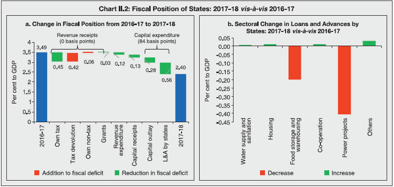
| Table II.2: Aggregate Receipts of State Governments and UTs | | (₹ lakh crore) | | Item | 2015-16 | 2016-17 | 2017-18 | 2018-19 (RE) | 2019-20 (BE) | | 1 | 2 | 3 | 4 | 5 | 6 | | Aggregate Receipts (1+2) | 22.99 | 26.47 | 27.76 | 34.29 | 37.63 | | (16.8) | (17.3) | (16.3) | (18.1) | (17.7) | | 1. Revenue Receipts (a+b) | 18.73 | 20.86 | 23.21 | 28.62 | 31.54 | | (13.6) | (13.6) | (13.6) | (15.1) | (14.9) | | a. States' Own Revenue (i+ii) | 10.35 | 11.18 | 13.10 | 14.92 | 16.55 | | (7.5) | (7.3) | (7.7) | (7.8) | (7.8) | | i. States' Own Tax | 8.80 | 9.46 | 11.30 | 12.69 | 14.09 | | (6.4) | (6.2) | (6.6) | (6.7) | (6.7) | | ii. States' Own Non-Tax | 1.55 | 1.71 | 1.80 | 2.23 | 2.45 | | (1.1) | (1.1) | (1.1) | (1.2) | (1.2) | | b. Central Transfers (i+ii) | 8.38 | 9.69 | 10.11 | 13.70 | 15.00 | | (6.1) | (6.3) | (5.9) | (7.2) | (7.1) | | i. Tax Devolution | 5.06 | 6.08 | 6.05 | 7.59 | 8.52 | | (3.7) | (4.0) | (3.5) | (4.0) | (4.0) | | ii. Grants-in Aid | 3.32 | 3.61 | 4.06 | 6.11 | 6.48 | | | (2.4) | (2.3) | (2.4) | (3.2) | (3.1) | | 2. Net Capital Receipts (a+b) | 4.26 | 5.61 | 4.55 | 5.67 | 5.99 | | (3.2) | (3.7) | (2.6) | (3.0) | (2.8) | | a. Non-Debt Capital Receipts | 0.08 | 0.16 | 0.40 | 0.52 | 0.62 | | (0.1) | (0.1) | (0.2) | (0.3) | (0.3) | | i. Recovery of Loans and Advances | 0.07 | 0.16 | 0.40 | 0.52 | 0.60 | | (0.1) | (0.1) | (0.2) | (0.3) | (0.3) | | ii. Miscellaneous Capital Receipts | 0.01 | 0.00 | 0.00 | 0.00 | 0.02 | | (0.0) | (0.0) | (0.0) | (0.0) | (0.0) | | b. Debt Receipts | 4.18 | 5.45 | 4.15 | 5.15 | 5.37 | | (3.1) | (3.6) | (2.4) | (2.8) | (2.5) | | i. Market Borrowings | 2.59 | 3.52 | 3.45 | 4.09 | 4.86 | | (1.9) | (2.3) | (2.0) | (2.2) | (2.3) | | ii. Other Debt Receipts | 1.59 | 1.93 | 0.70 | 1.06 | 0.51 | | | (1.2) | (1.3) | (0.4) | (0.6) | (0.2) | RE: Revised Estimates. BE: Budget Estimates.
Note: 1. Figures in parentheses are percent of GDP.
2. Debt receipts are on net basis.
Source: Budget documents of state governments. | 2.6 The decline in revenue expenditure was largely driven by lower spending on education, power and relief on account of natural calamities, even as non-development expenditure increased due to higher interest and pension payments; states increased revenue spending on crop husbandry and different agricultural programmes (Table II.3). 2.7 Summing up, non-development expenditure rose sharply during 2017-18 in a break from the past. On the other hand, development expenditure suffered erosion indicating that the quality of expenditure was compromised by a combination of higher revenue expenditure and lower capital expenditure. 3. Revised Estimates: 2018-19 2.8 As per the revised estimates for 2018-19, states’ fiscal deficit at 2.9 per cent of GDP was higher by 34 basis points than the budget estimates (BE). This was primarily due to lower than budgeted receipts and higher expenditure, particularly in the revenue account accruing mainly from farm loan waiver, both new announcements and existing schemes and farmer income support schemes (Box II.1). 
| Table II.3: Expenditure Pattern of State Governments and UTs | | (₹ lakh crore) | | Item | 2015-16 | 2016-17 | 2017-18 | 2018-19 (RE) | 2019-20 (BE) | | 1 | 2 | 3 | 4 | 5 | 6 | | Aggregate Expenditure (1+2 = 3+4+5) | 23.01 | 26.38 | 27.72 | 34.70 | 37.68 | | | (16.7) | (17.2) | (16.2) | (18.3) | (17.9) | | 1. Revenue Expenditure | 18.70 | 21.22 | 23.40 | 28.75 | 31.46 | | of which: | (13.6) | (13.8) | (13.7) | (15.1) | (14.9) | | Interest Payments | 2.18 | 2.55 | 2.93 | 3.20 | 3.55 | | | (1.6) | (1.7) | (1.7) | (1.7) | (1.7) | | 2. Capital Expenditure | 4.31 | 5.17 | 4.31 | 5.95 | 6.22 | | of which: | (3.1) | (3.4) | (2.5) | (3.1) | (2.9) | | Capital Outlay | 3.39 | 3.96 | 3.94 | 5.44 | 5.81 | | | (2.5) | (2.6) | (2.3) | (2.9) | (2.8) | | 3. Development Expenditure | 16.14 | 18.62 | 18.77 | 24.04 | 25.75 | | | (11.7) | (12.1) | (11.0) | (12.6) | (12.2) | | 4. Non-Development Expenditure | 6.38 | 7.20 | 8.26 | 9.84 | 10.98 | | | (4.6) | (4.7) | (4.8) | (5.2) | (5.2) | | 5. Others* | 0.49 | 0.56 | 0.68 | 0.82 | 0.95 | | | (0.4) | (0.4) | (0.4) | (0.4) | (0.4) | RE: Revised Estimates. BE: Budget Estimates.
*: Includes grants-in-aid and contributions (compensation and assignments to local bodies).
Note: 1. Figures in parentheses are percent to GDP.
2. Capital expenditure includes capital outlay and loans and advances by state governments.
Source: Budget documents of state governments. |
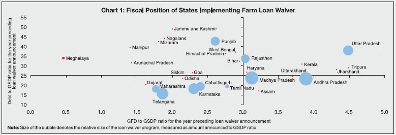
Box II.1: Farm Loan Waivers and Income Support Schemes Since 2014-15, 10 states have announced loan waiver programmes of an aggregate amount of ₹2.3 lakh crore (1.4 per cent of GDP), significantly higher than the previous two nation-wide debt waiver programmes — ₹10,000 crore in 19902 and ₹52,500 crore in 2007-083. The economic rationale for loan waivers is to alleviate the debt overhang of beneficiaries to enable them to undertake productive investment and boost real economic activity (RBI, 2019). States like Rajasthan, Madhya Pradesh and Chhattisgarh announced new loan waiver programmes in 2018-19 to the tune of ₹18,000 crore (1.9 per cent of GSDP), ₹36,500 crore (4.5 per cent of GSDP) and ₹6,100 crore (1.7 per cent of state GSDP), respectively. Karnataka expanded its loan waiver programme from ₹18,000 crore announced in 2017-18 to ₹44,000 crore (3.4 per cent of GSDP) in 2018-19. The impact of loan waivers on states’ budgets is typically staggered over three to five years, either due to phased rollouts or by clearing bank dues over multi-year pay-outs. This impact varies widely across states, ranging between 0.1 per cent of GSDP in Andhra Pradesh and Tamil Nadu to 1.8 per cent of GSDP in Chhattisgarh in 2018-19. In the 2019-20 (BE), states have allocated between 0.1 to 2.0 per cent of GSDP to farm loan waivers (Table 1). Eight out of the ten states that announced loan waivers appear to have fiscal space to accommodate them in terms of debt levels relative to the average, though it might pose risks to the finances of some states (Chart 1). Sharp deceleration in growth of agricultural credit outstanding and declined agricultural credit disbursements has been observed in the years of loan waiver programmes, with growth bouncing back in subsequent years (Chart 2). Farm loan waivers have also come under increasing scrutiny in the wake of their adverse impact on credit culture due to moral hazard among both beneficiaries and non-beneficiaries of the bail out (RBI, 2019). Thus, as an alternative, income support schemes for farmers were for the first time announced by some state governments in 2018-19. The defining feature of income support schemes is that they provide cash transfers to farmers which are not linked to volume of production, factor of production employed and prices. Accordingly, they are categorised as Green Box payments under the Agreement on Agriculture of the World Trade Organisation (WTO) (Bhaskar et al., 2009). Telangana was the first state to announce income support scheme for farmers. In 2019-20, six states have budgeted an allocation for income support schemes, which is over and above Pradhan Mantri Kisan Samman Nidhi (PM-KISAN) scheme of the Union Government (Table 2)4. | Table 1: Fiscal Impact of States’ Farm Loan Waiver Programs | | (₹ crore) | | State | Year of Announcement | Amount Announced | Amount Provided in the Budget | | 2014-15 | 2015-16 | 2016-17 | 2017-18 | 2018-19 RE | 2019-20 BE | | 1 | 2 | 3 | 4 | 5 | 6 | 7 | 8 | 9 | | 1. Andhra Pradesh | 2014-15 | 24,000 | 4,000 | 742 | 3,512 | 3,602 | 875 | | | | | | (0.9) | (0.1) | (0.6) | (0.6) | (0.1) | | | 2. Telangana | 2014-15 | 17,000 | 4,250 | 4,250 | 2,957 | 4,016 | | 6,000 | | | | | (1.0) | (0.9) | (0.6) | (0.7) | | (0.9) | | 3. Tamil Nadu | 2016-17 | 5,280 | | | 1,682 | 1,870 | 884 | 807 | | | | | | | (0.2) | (0.2) | (0.1) | (0.1) | | 4. Maharashtra | 2017-18 | 34,020 | | | | 15,020 | 6,500 | 405 | | | | | | | | (0.8) | (0.3) | (0.0) | | 5. Uttar Pradesh | 2017-18 | 36,360 | | | | 21,102 | 5,500 | 600 | | | | | | | | (2.0) | (0.5) | (0.1) | | 6. Punjab | 2017-18 | 10,000 | | | | 348 | 5,500 | 3,000 | | | | | | | | (0.1) | (1.4) | (0.7) | | 7. Karnataka | 2018-19 | 44,000 | | | | 3,917 | 11,965 | 12,650 | | | | | | | | (0.4) | (1.1) | (1.0) | | 8. Rajasthan | 2018-19 | 18,000 | | | | | 3,000 | 3,240 | | | | | | | | | (0.4) | (0.4) | | 9. Madhya Pradesh | 2018-19 | 36,500 | | | | | 5,000 | 8,000 | | | | | | | | | (0.9) | (1.4) | | 10. Chhattisgarh | 2018-19 | 6,100 | | | | | 4,223 | 5,000 | | | | | | | | | (1.8) | (2.0) | | Total | | 2,31,260 | 8,250 | 4,992 | 8,151 | 49,875 | 43,447 | 39,703 | | As per cent of state governments’ total expenditure | 0.4 | 0.2 | 0.3 | 1.8 | 1.2 | 1.2 | | As per cent to GDP | 0.1 | 0.0 | 0.1 | 0.3 | 0.2 | 0.2 | Note: Figures in parentheses indicate loan waiver as a per cent to respective states GSDP for the corresponding year.
Sources: State governments, Budget documents of state governments. |
 The year 2018-19, thus, marks a watershed, with some state governments opting for income support schemes as the preferred policy tool over conventional policies like enhancing minimum support prices (MSP) and farm loan waivers to alleviate agricultural distress. While the broad objective of all the three policies is to stabilise farmers’ incomes, income support schemes have certain advantages over the rest. First, income support schemes are more inclusive as even landless farmers and farmers having no access to bank credit can be covered, whereas farm loan waivers benefit only those farmers who have borrowed from banks. Second, the problem of moral hazard, which is typically associated with farm loan waivers, does not exist in the case of income support schemes. Furthermore, direct benefit transfers are the fastest and most effective way to reach farmers, by contrast, benefits of Minimum Support Prices (MSPs) reach the farmers only indirectly and are mostly appropriated by traders who bring the produce to the market (Gulati et al., 2018). However, critical for their success is digitisation of land records and their seeding with bank account and Aadhaar details for ensuring timely payments to farmers while minimising inclusion and exclusion errors. | Table 2: Income Support Schemes Announced by State Governments | | (₹ crore) | | State | Name of the Scheme | 2018-19 (BE) | 2018-19 (RE) | 2019-20 (BE) | | 1 | 2 | 3 | 4 | 5 | | 1. Andhra Pradesh | YSR Rythu Bharosa | - | - | 8,750 | | 2. Haryana | Mukhyamantri Parivar Samman Nidhi | - | - | 1,500 | | 3. Jharkhand | Mukhyamantri Krishi Ashirvad Yojana | - | - | 2,000 | | 4. Karnataka | - | 1,000 | 270 | 0 | | 5. Odisha | Krushak Assistance for Livelihood and Income Augmentation (KALIA) | 250 | 250 | 5,611 | | 6. Telangana | Rythu Bandhu | 12,000 | 12,000 | 12,000 | | 7. West Bengal | Krishak Bandhu | - | 4,000 | 3,000 | | Total | 13,250 | 16,520 | 32,861 | | As per cent of state governments’ total expenditure | 0.4 | 0.5 | 0.9 | | As per cent of GDP | 0.1 | 0.1 | 0.2 | | - : Not available |
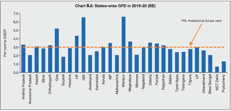
References: Bhaskar, A., & Beghin, J. (2009). “How Coupled Are Decoupled Farm Payments? A Review of the Evidence”. Journal of Agricultural and Resource Economics, 34(1). Gulati, A., Chatterjee, T., & Hussain, S. (2018). “Supporting Indian Farmers: Price Support or Direct Income/Investment Support?”. Indian Council for Research on International Economic Relations (ICRIER) Working Paper No. 357. RBI (2019), “Report of the Internal Working Group to Review Agricultural Credit”. Reserve Bank of India. | 2.9 While developmental expenditure reversed the decline recorded in the preceding year, non-developmental expenditure rose in 2018-19 (RE) continuing the trend from 2017-18 primarily led by committed expenditures in the form of pension payments and administrative services (Chart II.4). 2.10 Revised Estimates usually get revised downward when they crystallise into accounts (Chart II.5). Accounts data, available with Comptroller and Auditor General of India (CAG), provide a close assessment of actual accounts, albeit with lower granularity.5 2.11 In terms of these provisional accounts (PA), the consolidated GFD at 2.4 per cent of GDP in 2018-19 remained almost the same (only 3 basis points higher) as in 2017-18, affirming that states have stayed on the course of fiscal consolidation (Table II.4). 4. Budget Estimates: 2019-20 2.12 States have budgeted a GFD-GDP ratio of 2.6 per cent in 2019-20, with 12 states expecting to remain above 3 per cent (Table II.5, Chart II.6). As in budget estimates of the previous few years, a combined revenue surplus is budgeted for 2019-20, with 19 states and UTs expecting surplus. | Table II.4: Fiscal Position of States | | (₹ lakh crore) | | | 2017-18 | 2018-19 (RE) | 2018-19 (PA) | 2019-20 (BE) | | 1 | 2 | 3 | 4 | 5 | | I. Aggregate Receipts | 23.61 | 29.14 | 26.68 | 32.16 | | | (13.8) | (15.4) | (14.0) | (15.2) | | A. Revenue Receipts | 23.21 | 28.62 | 26.23 | 31.54 | | | (13.6) | (15.1) | (13.8) | (14.9) | | B. Capital Receipts | 0.40 | 0.52 | 0.45 | 0.62 | | | (0.2) | (0.3) | (0.2) | (0.3) | | a. Recovery of Loans and Advances | 0.40 | 0.52 | 0.45 | 0.60 | | | (0.2) | (0.3) | (0.2) | (0.3) | | b. Other Receipts | 0.00 | 0.00 | 0.01 | 0.02 | | | (0.0) | (0.0) | (0.0) | (0.0) | | II. Aggregate Expenditure | 27.71 | 34.70 | 31.31 | 37.68 | | | (16.2) | (18.2) | (16.5) | (17.8) | | A. Revenue Expenditure | 23.40 | 28.75 | 26.36 | 31.46 | | | (13.7) | (15.1) | (13.9) | (14.9) | | B. Capital Expenditure | 4.31 | 5.95 | 4.95 | 6.22 | | | (2.5) | (3.1) | (2.6) | (2.9) | | a. Capital Outlay | 3.94 | 5.44 | 4.50 | 5.81 | | | (2.3) | (2.9) | (2.4) | (2.8) | | b. Loans and Advances by States | 0.37 | 0.51 | 0.45 | 0.41 | | | (0.2) | (0.2) | (0.2) | (0.1) | | III. Fiscal Deficit/Surplus | 4.10 | 5.55 | 4.62 | 5.52 | | | (2.4) | (2.9) | (2.4) | (2.6) | | IV. Revenue Deficit/surplus | 0.19 | 0.13 | 0.13 | -0.08 | | | (0.1) | (0.1) | (0.1) | (0.0) | * : While data on 27 states for 2018-19 (provisional estimates) are taken from CAG, data for Goa and Assam are based on the revised estimates given in their budget documents. Data for all states for 2017-18 are from budget documents of respective states.
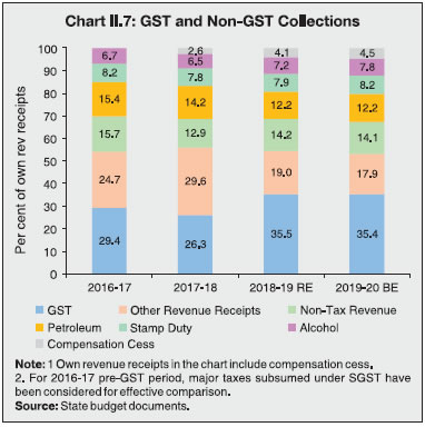
Note: Figures in parentheses are per cent of GDP. | Receipts 2.13 Growth in Revenue receipts is expected to decelerate in 2019-20, due to lower tax devolution and grants (Table II.6). State Goods and Services Tax (SGST) collections have risen from 29 per cent of states’ own revenue receipts in 2016-17 to 35 per cent in 2019-20 (BE)6. As these revenues have proved inadequate relative to rising expenditure, states adapted by shifting towards other sources of taxes, viz., alcohol and stamp duties. Notwithstanding a decline in the excise duty on petroleum in 2018, it accounted for above 11 per cent of states’ own tax revenues (Chart II.7). GST compensation provided by Centre has also increased since the implementation of GST. Furthermore, lower variability and enhanced predictability of income through these sources can play an important role in utilising these revenues in an effective and timely manner (Annex II.1). | Table II.5: Deficit Indicators of State Governments—State-wise | | (Per cent) | | | 2016-17 | 2017-18 | 2018-19 (RE) | 2019-20 (BE) | | RD/ GSDP | GFD/ GSDP | PD/ GSDP | RD/ GSDP | GFD/ GSDP | PD/ GSDP | RD/ GSDP | GFD/ GSDP | PD/ GSDP | RD/ GSDP | GFD/ GSDP | PD/ GSDP | | 1 | 2 | 3 | 4 | 5 | 6 | 7 | 8 | 9 | 10 | 11 | 12 | 13 | | 1. Andhra Pradesh | 2.5 | 4.4 | 2.8 | 2.0 | 4.0 | 2.3 | 1.2 | 3.6 | 2.1 | 0.2 | 3.3 | 1.7 | | 2. Arunachal Pradesh | -12.2 | -4.3 | -6.3 | -13.0 | 1.4 | -0.7 | -26.5 | 4.3 | 2.0 | -29.1 | 2.0 | -0.4 | | 3. Assam | 0.1 | 2.4 | 1.2 | 0.5 | 3.2 | 2.1 | -2.4 | 3.0 | 1.7 | -0.9 | 3.1 | 1.7 | | 4. Bihar | -2.6 | 3.9 | 2.0 | -3.1 | 3.0 | 1.1 | -1.7 | 4.6 | 2.6 | -3.8 | 2.8 | 0.9 | | 5. Chhattisgarh | -2.2 | 1.6 | 0.5 | -1.2 | 2.4 | 1.3 | 2.0 | 6.0 | 4.8 | -0.3 | 3.2 | 1.8 | | 6. Goa | -1.1 | 1.5 | -0.3 | -0.7 | 2.3 | 0.5 | -0.2 | 5.3 | 3.6 | -0.5 | 5.2 | 3.4 | | 7. Gujarat | -0.5 | 1.4 | -0.1 | -0.4 | 1.6 | 0.2 | -0.1 | 2.1 | 0.8 | -0.2 | 1.8 | 0.6 | | 8. Haryana | 2.9 | 4.7 | 2.8 | 1.7 | 3.1 | 1.1 | 1.2 | 2.9 | 0.9 | 1.5 | 2.9 | 0.7 | | 9. Himachal Pradesh | -0.7 | 4.6 | 2.0 | -0.2 | 2.8 | 0.1 | 1.4 | 5.1 | 2.4 | 1.4 | 4.4 | 1.7 | | 10. Jammu and Kashmir | -1.7 | 4.9 | 1.3 | -5.5 | 2.0 | -1.4 | -5.1 | 11.2 | 7.6 | -7.9 | 6.5 | 2.4 | | 11. Jharkhand | -0.8 | 4.3 | 2.5 | -0.7 | 4.3 | 2.6 | -2.3 | 2.4 | 0.7 | -2.4 | 2.0 | 0.6 | | 12. Karnataka | -0.1 | 2.4 | 1.4 | -0.3 | 2.3 | 1.3 | 0.0 | 2.9 | 1.7 | 0.0 | 2.5 | 1.4 | | 13. Kerala | 2.4 | 4.2 | 2.3 | 2.4 | 3.8 | 1.7 | 1.7 | 3.0 | 1.0 | 1.0 | 3.0 | 1.0 | | 14. Madhya Pradesh | -0.6 | 4.3 | 2.9 | -0.6 | 3.1 | 1.6 | 0.0 | 3.5 | 2.0 | -0.1 | 3.5 | 1.9 | | 15. Maharashtra | 0.4 | 1.8 | 0.5 | -0.1 | 1.0 | -0.4 | 0.6 | 2.1 | 0.8 | 0.7 | 2.0 | 0.8 | | 16. Manipur | -4.4 | 2.6 | 0.0 | -4.5 | 1.4 | -0.9 | 0.0 | 11.9 | 9.5 | -1.3 | 6.6 | 4.3 | | 17. Meghalaya | -2.2 | 2.5 | 0.6 | -2.8 | 0.5 | -1.5 | -1.5 | 3.5 | 1.5 | -2.0 | 3.6 | 1.6 | | 18. Mizoram | -6.8 | -1.5 | -3.5 | -9.6 | 1.8 | -0.1 | -2.4 | 7.6 | 5.8 | -5.6 | 2.1 | 0.7 | | 19. Nagaland | -3.6 | 1.4 | -1.6 | -3.5 | 1.9 | -1.0 | -2.0 | 5.1 | 2.1 | -1.8 | 3.0 | -0.1 | | 20. Odisha | -2.4 | 2.4 | 1.4 | -3.1 | 2.1 | 1.0 | -2.2 | 2.9 | 1.7 | -1.2 | 3.5 | 2.3 | | 21. Punjab | 1.7 | 12.4 | 9.6 | 2.0 | 2.6 | -0.6 | 2.3 | 3.4 | 0.3 | 2.0 | 3.4 | 0.3 | | 22. Rajasthan | 2.4 | 6.1 | 3.8 | 2.2 | 3.0 | 0.7 | 2.7 | 3.4 | 1.0 | 2.6 | 3.2 | 0.9 | | 23. Sikkim | -4.0 | -0.4 | -2.0 | -4.5 | 2.0 | 0.4 | -3.3 | 3.4 | 1.7 | -0.9 | 2.8 | 1.0 | | 24. Tamil Nadu | 1.0 | 4.3 | 2.7 | 1.5 | 2.7 | 0.9 | 1.2 | 2.7 | 1.0 | 0.8 | 2.4 | 0.6 | | 25. Telangana | -0.2 | 5.3 | 4.0 | -0.5 | 3.5 | 2.1 | 0.0 | 3.3 | 2.0 | -0.2 | 2.4 | 1.0 | | 26. Tripura | -2.3 | 6.1 | 4.1 | 0.6 | 4.5 | 2.6 | -3.2 | 2.1 | 0.5 | -1.6 | 2.8 | 1.2 | | 27. Uttar Pradesh | -1.6 | 4.5 | 2.3 | -0.9 | 2.0 | -0.1 | -3.2 | 3.0 | 0.8 | -1.8 | 3.0 | 0.7 | | 28. Uttarakhand | 0.2 | 2.8 | 0.9 | 0.9 | 3.7 | 1.8 | 0.0 | 2.3 | 0.2 | 0.0 | 2.6 | 0.6 | | 29. West Bengal | 1.8 | 2.9 | 0.0 | 1.0 | 2.9 | 0.1 | 0.6 | 2.8 | 0.3 | 0.0 | 2.0 | -0.3 | | 30. NCT Delhi | -0.8 | 0.2 | -0.3 | -0.7 | 0.0 | -0.4 | -0.6 | 0.1 | -0.3 | -0.6 | 0.7 | 0.3 | | 31. Puducherry | 0.3 | 1.8 | -0.2 | -0.6 | 0.6 | -1.5 | -0.1 | 1.1 | -0.8 | 0.0 | 1.3 | -1.0 | | All States | 0.2 | 3.5 | 1.8 | 0.1 | 2.4 | 0.7 | 0.1 | 2.9 | 1.2 | 0.0 | 2.6 | 0.9 | RE: Revised Estimates. BE: Budget Estimates. RD: Revenue Deficit. GFD : Gross Fiscal Deficit.
PD: Primary Deficit. GSDP: Gross State Domestic Product.
Note: Negative (-) sign in deficit indicators indicates surplus.
Source: Based on budget documents of state governments. |
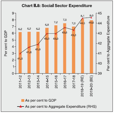
 Expenditure 2.14 Lower increase in revenue expenditure is envisaged in 2019-20 (vis-à-vis 2018-19 RE) except on roads and bridges and other agricultural programmes under developmental expenditures and interest payments under non-developmental expenditures (Table II.6). Capital outlay is expected to slow to 6.9 per cent from 38.1 per cent in the previous year. Given high capital expenditure multiplier, it is important that states meet the budgeted target and front-load these expenditure. However, capital outlay remained strong with a growth of 30.6 per cent during 2019-20 when compared with provisional accounts data of CAG for 2018-19 (Table II.4). 2.15 After witnessing a fall in 2017-18, social sector expenditure recovered in 2018-19 and is budgeted to sustain this improvement and reach to 8.0 per cent of GDP in 2019-20 (Chart II.8). | Table II.6: Variation in Major Items | | (₹ lakh crore) | | Item | 2015-16 | 2016-17 | 2017-18 | 2018-19 (RE) | 2019-20 (BE) | Per cent Variation | | 2018-19 RE over 2017-18 | 2019-20 BE over 2018-19RE | | 1 | 2 | 3 | 4 | 5 | 6 | 7 | 8 | | I. Revenue Receipts (i+ii) | 18.73 | 20.86 | 23.21 | 28.62 | 31.54 | 23.3 | 10.2 | | (i) Tax Revenue (a+b) | 13.86 | 15.54 | 17.36 | 20.28 | 22.61 | 16.8 | 11.5 | | (a) Own Tax Revenue | 8.80 | 9.46 | 11.30 | 12.69 | 14.09 | 12.2 | 11.1 | | of which: Sales Tax | 5.50 | 6.10 | 4.02 | 2.97 | 3.26 | -26.1 | 10.0 | | (b) Share in Central Taxes | 5.06 | 6.08 | 6.05 | 7.59 | 8.52 | 25.5 | 12.1 | (ii) Non-Tax Revenue | 4.87 | 5.32 | 5.86 | 8.34 | 8.93 | 42.4 | 7.1 | | (a) States’ Own Non-Tax Revenue | 1.55 | 1.71 | 1.80 | 2.23 | 2.45 | 24.2 | 9.9 | | (b) Grants from Centre | 3.32 | 3.61 | 4.06 | 6.11 | 6.48 | 50.5 | 6.1 | | II. Revenue Expenditure | 18.70 | 21.22 | 23.40 | 28.75 | 31.46 | 22.9 | 9.4 | | of which: | | | | | | | | | (i) Development Expenditure | 12.04 | 13.66 | 14.66 | 18.42 | 19.96 | 25.7 | 8.3 | | of which: | | | | | | | | | Education, Sports, Art and Culture | 3.57 | 3.95 | 4.25 | 5.12 | 5.68 | 20.6 | 10.9 | | Transport and Communication | 0.43 | 0.48 | 0.51 | 0.52 | 0.55 | 2.4 | 5.9 | | Power | 1.12 | 1.33 | 1.16 | 1.32 | 1.47 | 13.1 | 11.9 | | Relief on account of Natural Calamities | 0.33 | 0.28 | 0.16 | 0.37 | 0.29 | 132.8 | -22.4 | | Rural Development | 1.08 | 1.26 | 1.32 | 1.68 | 1.83 | 27.1 | 8.7 | | (ii) Non-Development Expenditure | 6.17 | 6.99 | 8.06 | 9.50 | 10.55 | 17.9 | 11.0 | | of which: | | | | | | | | | Administrative Services | 1.32 | 1.47 | 1.62 | 1.99 | 2.22 | 22.7 | 11.8 | | Pension | 2.05 | 2.27 | 2.75 | 3.16 | 3.47 | 14.8 | 9.7 | | Interest Payments | 2.18 | 2.55 | 2.93 | 3.20 | 3.55 | 9.0 | 11.0 | | III. Net Capital Receipts # | 4.26 | 5.61 | 4.54 | 5.66 | 6.01 | 24.9 | 5.4 | | of which: | | | | | | | | | Non-Debt Capital Receipts | 0.08 | 0.16 | 0.40 | 0.52 | 0.62 | 31.3 | 18.1 | | IV. Capital Expenditure $ | 4.31 | 5.17 | 4.31 | 5.95 | 6.22 | 37.9 | 4.6 | | of which: | | | | | | | | | Capital Outlay | 3.39 | 3.96 | 3.94 | 5.44 | 5.81 | 38.1 | 6.9 | | of which: | | | | | | | | | Capital Outlay on Irrigation and Flood Control | 0.69 | 0.83 | 0.83 | 1.10 | 1.01 | 33.1 | -7.7 | | Capital Outlay on Energy | 0.47 | 0.53 | 0.46 | 0.54 | 0.55 | 15.3 | 3.0 | | Capital Outlay on Transport | 0.81 | 0.96 | 0.93 | 1.23 | 1.22 | 32.2 | -1.1 | | Memo Item: | | | | | | | | | Revenue Deficit | -0.03 | 0.36 | 0.19 | 0.13 | -0.08 | -32.1 | -163.4 | | Gross Fiscal Deficit | 4.20 | 5.36 | 4.10 | 5.55 | 5.52 | 35.3 | -0.5 | | Primary Deficit | 2.02 | 2.81 | 1.17 | 2.36 | 1.98 | 101.0 | -16.3 | RE: Revised Estimates. BE: Budget Estimates.
# : It includes following items on net basis: Internal Debt, Loans and Advances from the Centre, Inter-State Settlement, Contingency Fund, Small Savings, Provident Funds, etc, Reserve Funds, Deposits and Advances, Suspense and Miscellaneous, Appropriation to Contingency Fund and Remittances.
$ : Capital Expenditure includes Capital Outlay and Loans and Advances by State Governments.
Note: 1. Negative (-) sign in deficit indicators implies surplus.
2. Also see Notes to Appendices.
Source: Budget documents of state governments. |
 2.16 Compositionally, a shift is projected from expenditure on education, health and family welfare to sectors like housing and urban development and expenditure on social security and welfare (Table II.7). Recent initiatives by the Centre like Ayushman Bharat may impact social sector expenditures in the area of health going forward (Box II.2). 5. Financing and Market Borrowing 2.17 Market borrowings financed 52.8 per cent of the combined fiscal deficit of states during 2001-02 to 2016-17. Since 2017-18, the share of market borrowings in financing the GFD has increased rapidly and is expected to increase to 88 per cent during 2019-20 (BE) (Table II.8). States with GFD equal to or less than 3.0 per cent have financed it entirely through market borrowings. States with GFD-GDP ratios of more than 3 per cent have relied on other sources, viz., provident funds, deposit and advances and cash withdrawals. 2.18 Comparing with Centre, states’ borrowings are increasingly getting channelised towards capital outlays which augurs well for long-term growth (Chart II. 9a). A similar trend is observed in the ratio of revenue expenditure to capital expenditure (a proxy for quality of expenditure) for Centre and states, i.e., deterioration in 2017-18 and likely improvement in 2018-19 (Chart II.9b). Table II.7: Composition of Expenditure on Social Services
(Revenue and Capital Accounts) | | (Per cent to expenditure on social services) | | Item | 2015-16 | 2016-17 | 2017-18 | 2018-19 (RE) | 2019-20 (BE) | | 1 | 2 | 3 | 4 | 5 | 6 | | Expenditure on Social Services (a to l) | 100.0 | 100.0 | 100.0 | 100.0 | 100.0 | | (a) Education, Sports, Art and Culture | 44.0 | 43.0 | 42.9 | 40.5 | 41.5 | | (b) Medical and Public Health | 11.6 | 11.8 | 12.3 | 11.9 | 11.8 | | (c) Family Welfare | 2.0 | 1.9 | 2.0 | 2.0 | 2.0 | | (d) Water Supply and Sanitation | 6.1 | 6.5 | 7.0 | 6.5 | 6.7 | | (e) Housing | 2.9 | 3.2 | 3.8 | 4.5 | 3.8 | | (f) Urban Development | 6.5 | 8.0 | 7.6 | 8.7 | 8.8 | | (g) Welfare of SCs, STs and OBCs | 7.0 | 6.9 | 7.4 | 7.0 | 6.9 | | (h) Labour and Labour Welfare | 0.9 | 0.8 | 0.9 | 1.0 | 1.1 | | (i) Social Security and Welfare | 11.4 | 10.9 | 10.4 | 11.5 | 11.6 | | (j) Nutrition | 2.6 | 2.4 | 2.3 | 2.2 | 2.2 | | (k) Expenditure on Natural Calamities | 3.9 | 2.9 | 1.6 | 2.8 | 2.0 | | (l) Others | 1.1 | 1.6 | 1.8 | 1.5 | 1.5 | RE: Revised Estimates. BE: Budget Estimates.
Source : Budget documents of the state governments. |
Box II.2: Ayushman Bharat Programme With an aim to safeguard the poor from the catastrophic effects of high out of pocket (OOP) expenditure, which characterises health spending in India (Chart 1), the Ayushman Bharat programme was announced on February 1, 2018. Ayushman Bharat is an umbrella of two major health initiatives (i) Ayushman Bharat - Health and Wellness Centres (AB-HWC) which aims to transform nearly 1.5 lakh sub-centres and primary health centres into HWCs providing comprehensive and quality primary care; (ii) Ayushman Bharat - Pradhan Mantri Jan Arogya Yojana (AB-PMJAY), under which 10.74 crore poor and deprived rural families and identified occupational categories of urban workers’ families will be provided a cover of ₹5 lakh per family per year for in-patient secondary and tertiary treatment. It is a centrally sponsored scheme, which will be implemented on a 60:40 sharing basis with states7. With a few exceptions, most states have signed up for AB-PMJAY. The Union Government has budgeted ₹2,400 crore and ₹6,400 crore in 2018-19 and 2019-20 respectively for the AB-PMJAY. The current allocation for AB-PMJAY by various states seems modest at 0.02 per cent of GDP (Chart 2). Even before the Ayushman Bharat programme was launched, a plethora of government funded health insurance schemes (GFHIS) were operational in India, like the Rashtriya Swasthya Bima Yojana (RSBY) of the Central government, Rajiv Arogyasri scheme of Telangana government, Arogya Bhagya scheme of Karnataka government, among others (Annex II.2). An analysis of these pre-existing GFHISs suggests that their net incurred claims ratio (NICR)8, which is an indicator of sustainability, has crossed 100 per cent, which means that insurance pay-outs are higher than the premium collected (Patnaik et al., 2018). Thus, the true fiscal cost for states and the Centre could be higher if the insurance companies become insolvent and require bail-outs.
References: GoI (2018, September 22). Ayushman Bharat –Pradhan Mantri Jan AarogyaYojana (AB-PMJAY). Retrieved September 23, 2019, from Press Information Bureau: https://pib.gov.in/Pressreleaseshare.aspx?PRID=1546948. Patnaik, I., Roy, S., & Shah, A. (2018). “The Rise of Government-funded Health Insurance in India”. National Institute of Public Finance and Policy (NIPFP) Working Paper No. 231. |
| Table II.8: Financing Pattern of Gross Fiscal Deficit | | Item | 2015-16 | 2016-17 | 2017-18 | 2018-19 (RE) | 2019-20 (BE) | 2017-18#
(Per cent to GDP/GSDP) | | GFD<=3.0 per cent | GFD> 3.0 per cent | All States/ UTs | | 1 | 2 | 3 | 4 | 5 | 6 | 7 | 8 | 9 | | Financing (1 to 8) | 100.0 | 100.0 | 100.0 | 100.0 | 100.0 | 2.0 | 3.5 | 2.4 | | 1. Market Borrowings | 61.6 | 65.7 | 84.0 | 73.7 | 87.9 | 2.0 | 2.4 | 2.0 | | 2. Loans from Centre | 0.4 | 1.0 | 1.1 | 2.6 | 3.3 | 0.0 | 0.0 | 0.0 | | 3. Special Securities issued to NSSF/Small Savings | 6.5 | -6.0 | -7.9 | -6.1 | -6.3 | -0.3 | -0.1 | -0.2 | | 4. Loans from LIC, NABARD, NCDC, SBI and Other Banks | 3.9 | 8.1 | 3.1 | 4.3 | 5.0 | 0.1 | 0.1 | 0.1 | | 5. Provident Fund | 7.9 | 7.4 | 8.2 | 6.3 | 5.9 | 0.1 | 0.3 | 0.2 | | 6. Reserve Funds | 0.1 | 3.9 | 0.9 | 3.1 | 2.8 | 0.1 | 0.0 | 0.0 | | 7. Deposits and Advances | 5.6 | 7.9 | 15.6 | 3.0 | 0.3 | 0.4 | 0.5 | 0.4 | | 8. Others | 14.1 | 11.9 | -5.1 | 13.1 | 1.2 | -0.3 | 0.3 | -0.1 | RE: Revised Estimates. BE: Budget Estimates.
NSSF: National Small Savings Fund; LIC: Life Insurance Corporation of India; NCDC: National Co-Operative Development Corporation; SBI: State Bank of India; NABARD: National Bank for Agriculture and Rural Development
#: Excludes Delhi and Puducherry.
Note : 1. See Notes to Appendix Table 9.
2. ‘Others’ include Compensation and Other Bonds, Loans from Other Institutions, Appropriation to Contingency Fund, Inter-State Settlement, Contingency Fund, Suspense and Miscellaneous, Remittance and Overall Surplus/Deficit.
Source : Budget documents of state governments. | 2.19 The Reserve Bank successfully managed the borrowing programme of the state governments during 2018-19, notwithstanding global headwinds and domestic challenges related to adhering to the glide path for reduction in securities held under Held to Maturity (HTM) category and the statutory liquidity ratio (SLR). The gross market borrowing of state governments increased by 14.1 per cent, while net borrowing increased by 2.4 per cent during 2018-19, indicating higher repayment liabilities. In 2018-19, there were 467 successful issuances, of which 59 were re-issuances, reflecting efforts by states towards consolidation of debt (Table II.9). 2.20 The weighted average yield (WAY) on SDLs stood at 8.32 per cent in 2018-19, up from 7.67 per cent in the previous year. WAY eased in the beginning of the year tracking the benchmark yield, with sentiments buoyed by several positive developments, viz., announcements of reduced market borrowings in the Union Budget along with the decision of the Centre not to front-load the issuances in H1:2018-19; and the RBI allowing banks to spread mark to market losses (MTM) incurred during Q3:2017-18 and Q4:2017-18. However, WAY rebounded with a hardening bias at end-April 2018 with the rise in international crude oil price, inflation concerns due to the revised formula of MSP, and rising trade protectionism. In H2:2018-19, SDL yields traded with a softening bias, supported by RBI announcements of multiple open market operations (OMOs), fall in crude oil prices, monetary policy easing through rate cuts, improvement of liquidity conditions, the announcements of voluntary retention route (VRR)9 for foreign portfolio investment (FPI) in debt, and benign inflation prints (Chart II.10). 
| Table II.9: Market Borrowings of States | | (₹ lakh crore) | | Item | 2016-17 | 2017-18 | 2018-19 | 2019-20* | | 1 | 2 | 3 | 4 | 5 | | 1. Maturities during the year | 0.39 | 0.79 | 1.30 | 0.58 | | 2. Gross sanction under article 293(3) | 4.00 | 4.82 | 5.50 | 5.14 | | 3. Gross amount raised during the year | 3.80 | 4.19 | 4.78 | 2.05 | | 4. Net amount raised during the year | 3.43 | 3.40 | 3.49 | 0.40 | | 5. Amount raised during the year to total Sanctions (per cent) | 96.0 | 87.0 | 87.0 | 39.88 | | 6. Weighted Average Yield of SDLs (cut-off) | 7.48 | 7.67 | 8.32 | 7.42 | | 7. Weighted Average Spread over corresponding G-Sec (bps) (cumulative) | 59 | 59 | 65 | 52 | | 8. Average Inter-State Yield Spread (bps) (for 10-year paper) | 7 | 6 | 6 | 4 | *: As on September 18, 2019.
Source: RBI. |
2.21 Despite this softening bias, the weighted average spread of SDL issuances over comparable Central Government Securities stood at 65 bps in 2018-19 as compared with 59 bps in 2017-18, reflecting liquidity premium. Maturity Pattern of State Government Securities 2.22 The maturity profile of states’ debt indicates that near to medium-term redemption pressures are likely to rise and reach a peak in 2026-27 (Chart II.11). At end-March 2019, 66.2 per cent of the outstanding SDLs was in the residual maturity bucket of five years and above (Table II.10). As 17.9 per cent of outstanding SDLs will mature in the next three years, redemption pressure is expected to rise in the medium term. Cash Management of State Governments 2.23 Developments highlighted so far suggest that the borrowing strategy of states should be aligned with their cash positions to avoid unwarranted interest burden and the negative carry on surplus cash investments (Chart II.12). 2.24 States have been accumulating sizeable cash surpluses in recent years in the form of Intermediate Treasury Bills (ITBs) and Auction Treasury Bills (ATBs). Outstanding investments in ITBs stood at ₹1.22 lakh crore at end-March 2019, while outstanding investments in ATBs stood at ₹0.74 lakh crore. 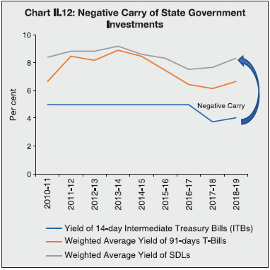
Table II.10: Maturity Profile of Outstanding State Government Securities
(As at end-March 2019) | | State | Per cent of Total Amount Outstanding | | 0-1 years | 1-3 years | 3-5 years | 5-7 years | Above 7 years | | 1 | 2 | 3 | 4 | 5 | 6 | | 1. Andhra Pradesh | 7.6 | 15.8 | 20.8 | 17.7 | 38.1 | | 2. Arunachal Pradesh | 2.6 | 1.1 | 13.3 | 14.5 | 68.5 | | 3. Assam | 6.3 | 9.2 | 8.2 | 20.0 | 56.5 | | 4. Bihar | 3.4 | 7.8 | 16.1 | 23.0 | 49.6 | | 5. Chhattisgarh | 1.7 | 13.9 | 23.2 | 29.6 | 31.6 | | 6. Goa | 5.4 | 7.7 | 16.7 | 20.4 | 49.7 | | 7. Gujarat | 5.7 | 16.2 | 16.3 | 16.3 | 45.5 | | 8. Haryana | 2.8 | 10.1 | 22.5 | 25.6 | 39.0 | | 9. Himachal Pradesh | 8.0 | 16.4 | 15.3 | 19.1 | 41.1 | | 10. Jammu & Kashmir | 3.2 | 18.8 | 14.3 | 12.6 | 51.0 | | 11. Jharkhand | 4.3 | 5.4 | 18.0 | 26.7 | 45.6 | | 12. Karnataka | 3.8 | 9.2 | 15.8 | 24.5 | 46.6 | | 13. Kerala | 4.2 | 11.1 | 18.8 | 21.7 | 44.2 | | 14. Madhya Pradesh | 5.5 | 12.6 | 13.2 | 24.9 | 43.8 | | 15. Maharashtra | 6.0 | 18.3 | 18.1 | 22.5 | 35.1 | | 16. Manipur | 10.6 | 8.6 | 13.2 | 22.5 | 45.0 | | 17. Meghalaya | 4.5 | 8.2 | 12.3 | 20.5 | 54.4 | | 18. Mizoram | 7.1 | 25.9 | 20.3 | 19.6 | 27.1 | | 19. Nagaland | 8.0 | 11.9 | 16.5 | 21.5 | 42.0 | | 20. Odisha | 3.6 | 21.3 | 25.5 | 10.7 | 38.9 | | 21. Punjab | 7.1 | 18.3 | 19.1 | 16.1 | 39.4 | | 22. Rajasthan | 7.4 | 13.4 | 15.8 | 21.6 | 41.8 | | 23. Sikkim | 7.4 | 0.9 | 7.0 | 20.6 | 64.0 | | 24. Tamil Nadu | 4.6 | 9.4 | 16.3 | 21.4 | 48.4 | | 25. Telangana | 0.0 | 0.0 | 1.7 | 22.9 | 75.4 | | 26. Tripura | 5.4 | 9.0 | 18.3 | 11.1 | 56.2 | | 27. Uttar Pradesh | 5.9 | 12.8 | 9.2 | 19.7 | 52.4 | | 28. Uttarakhand | 1.9 | 7.5 | 13.3 | 19.7 | 57.6 | | 29. West Bengal | 6.5 | 12.7 | 16.6 | 18.4 | 45.8 | | 30. Puducherry | 9.0 | 20.5 | 18.1 | 16.6 | 35.7 | | All States and UT | 5.3 | 12.6 | 16.0 | 20.8 | 45.4 | | Source: Reserve Bank records. |
| Table II.11: Investments of Surplus Cash balances of State Governments | | (₹ lakh crore) | | Item | Outstanding as on March 31 | | 2015-16 | 2016-17 | 2017-18 | 2018-19 | 2019-20* | | 1 | 2 | 3 | 4 | 5 | 6 | | 14-Day ITBs | 1.21 | 1.56 | 1.51 | 1.22 | 0.85 | | ATBs | 0.38 | 0.37 | 0.62 | 0.74 | 0.96 | | Total | 1.59 | 1.93 | 2.13 | 1.96 | 1.81 | *: As on September 17, 2019.
Source: RBI. | A few states have been parking sizeable cash balances in the more durable segment such as ATBs (Table II.11). Weekly auctions were also introduced with a view to even out cash flow mismatches while keeping the bare minimum cash balances. 2.25 Ways and Means Advances (WMA) limits are being fixed by a committee-based approach10. Following the recommendations of the Sumit Bose Committee, the limit of WMA for states was reviewed in 2018 and it was decided to retain the existing limit of WMA until reviewed by the next committee (effective from 2020-21). During 2018-19, 14 states resorted to WMA while 10 states availed overdraft (OD) vis-à-vis 13 states resorting to WMA and 7 states availing OD in 2017-18. Management of Reserve Funds of States 2.26 State governments maintain Consolidated Sinking Fund (CSF) and Guarantee Redemption Fund (GRF) with the Reserve Bank as buffer for repayment of their liabilities. States can avail of the Special Drawing Facility (SDF) at a discounted rate from the Reserve Bank against incremental funds invested in CSF and GRF as collateral. In order to incentivise adequate maintenance of these funds by the state governments and to encourage them to increase the corpus of these funds, the rate of interest on SDF was lowered from 100 bps below the repo rate to 200 bps below the repo rate in June 2018. Currently, 24 states are members of the CSF scheme while 18 states are members of the GRF scheme. Outstanding investment by states in the CSF and GRF as at end-March 2019 stood at ₹1.15 lakh crore and ₹0.07 lakh crore, respectively, as against ₹0.99 lakh crore and ₹0.05 lakh crore at end-March 2018 (Table II.12). | Table II.12: Investments in CSF/GRF by States | | (₹ crore) | | State/UT | CSF | GRF | CSF as per cent of Outstanding Liabilities | | 1 | 2 | 3 | 4 | | Andhra Pradesh | 7,459 | 735 | 3.0 | | Arunachal Pradesh | 1,027 | 1 | 13.4 | | Assam | 3,732 | 47 | 5.6 | | Bihar | 6,371 | 0 | 3.9 | | Chhattisgarh | 3,743 | 0 | 5.9 | | Goa | 539 | 270 | 2.8 | | Gujarat | 12,346 | 428 | 4.3 | | Haryana | 1,879 | 1,074 | 1.0 | | Karnataka | 3,466 | 0 | 1.3 | | Kerala | 1,942 | 0 | 0.8 | | Madhya Pradesh | 0 | 832 | 0.0 | | Maharashtra | 33,388 | 267 | 6.7 | | Manipur | 339 | 90 | 3.3 | | Meghalaya | 551 | 27 | 5.1 | | Mizoram | 497 | 29 | 6.3 | | Nagaland | 1,336 | 29 | 12.8 | | Odisha | 12,053 | 1,301 | 12.0 | | Punjab | 0 | 0 | 0.0 | | Rajasthan | 0 | 0 | 0.0 | | Tamil Nadu | 5,973 | 0 | 1.6 | | Telangana | 4,831 | 828 | 2.6 | | Tripura | 295 | 4 | 1.9 | | Uttar Pradesh | 0 | 0 | 0.0 | | Uttarakhand | 2,709 | 71 | 4.8 | | West Bengal | 9,938 | 479 | 2.5 | | Puducherry | 289 | 0 | 1.7 | | Total | 1,14,701 | 6,514 | 2.6 | 6. Outstanding Liabilities of State Governments 2.27 Outstanding liabilities of states have been growing at double digit rate since 2015-16 (except 2018-19), resulting in a rise in the debt to GDP ratios (Table II.13). Budget estimates suggest that 16 states and UTs expect to record higher debt-GSDP ratio in 2019-20 (Statement 20). 2.28 States’ outstanding debt rose for about a decade prior to 2003-04, but underwent a significant consolidation in the second phase post the adoption of FRL legislations by states (Chart II.13). As a result, the ratio of interest payment to revenue receipts (IP/RR) declined sharply during the period 2003-04 to 2014-15. Post the implementation of UDAY, however, states’ debt witnessed a significant rise in 2015-16 and 2016-17 and continued in 2017-18 albeit at a relatively lower rate despite ceasing of UDAY. This led to an increase in the interest payments to revenue receipts (IP/RR) ratio as well. Outstanding debt is expected to remain around 25 per cent of GDP as per the revised estimates for 2018-19 and budget estimates for 2019-20. | Table II.13: Outstanding Liabilities of State Governments and UTs | | Year | Amount | Annual Growth | Debt /GDP | | (End-March) | (₹ lakh crore) | (Per cent) | | 1 | 2 | 3 | 4 | | 2013 | 22.45 | 10.6 | 22.6 | | 2014 | 25.10 | 11.8 | 22.3 | | 2015 | 27.43 | 9.3 | 22.0 | | 2016 | 32.59 | 18.8 | 23.7 | | 2017 | 38.59 | 18.4 | 25.1 | | 2018 | 42.92 | 11.2 | 25.1 | | 2019 (RE) | 47.15 | 9.8 | 24.8 | | 2020 (BE) | 52.58 | 11.5 | 24.9 | RE: Revised Estimates. BE: Budget Estimates.
Source : 1. Budget documents of state governments.
2.Combined Finance and Revenue Accounts of the Union and the State Governments in India, Comptroller and Auditor General of India.
3.Ministry of Finance, Government of India.
4.Reserve Bank records.
5.Finance Accounts of the Union Government, Government of India. |
Composition of Debt 2.29 States’ dependence on market borrowing to finance their debt has increased significantly following the recommendation of the fourteenth Finance Commission (FC-XIV) to exclude states from the National Small Savings Fund (NSSF) financing facility (barring Delhi, Madhya Pradesh, Kerala and Arunachal Pradesh). All other components have witnessed a decline in the recent period (Table II.14). Table II.14: Composition of Outstanding Liabilities of State Governments
(As at end-March) | | (Per cent) | | Item | 2015 | 2016 | 2017 | 2018 | 2019 RE | 2020 BE | | 1 | 2 | 3 | 4 | 5 | 6 | 7 | | Total Liabilities (1 to 4) | 100.0 | 100.0 | 100.0 | 100.0 | 100.0 | 100.0 | | 1. Internal Debt | 70.0 | 72.1 | 73.3 | 72.7 | 73.3 | 74.8 | | of which: | | | | | | | | (i) Market Loans | 46.4 | 46.6 | 48.2 | 51.4 | 54.3 | 57.9 | | (ii) Special Securities Issued to NSSF | 19.8 | 17.5 | 14.0 | 11.1 | 9.4 | 7.7 | | (iii) Loans from Banks and Financial Institutions | 3.5 | 4.3 | 5.2 | 4.9 | 5.0 | 4.9 | | 2. Loans and Advances from the Centre | 5.5 | 4.7 | 4.1 | 3.8 | 3.7 | 3.7 | | 3. Public Account (i to iii) | 24.3 | 23.1 | 22.5 | 23.5 | 22.8 | 21.4 | | (i) State Provident Funds, etc. | 11.7 | 10.8 | 10.5 | 10.3 | 10.1 | 9.7 | | (ii) Reserve Funds | 3.6 | 4.3 | 3.2 | 4.1 | 4.1 | 4.0 | | (iii) Deposits and Advances | 9.0 | 8.0 | 8.8 | 9.1 | 8.6 | 7.8 | | 4. Contingency Fund | 0.2 | 0.1 | 0.1 | 0.1 | 0.1 | 0.1 | RE: Revised Estimate. BE: Budget Estimate.
Source: Same as that for Table II.13. | 7. Concluding Observations 2.30 To sum up, the GFD-GDP for states recorded improvement in 2017-18 (Accounts) vis-à-vis 2016-17 and remained well within the threshold of 3 per cent during 2018-19. A similar outcome is budgeted for 2019-20 (BE). There are, however, some important features of these budget outcomes which are noteworthy. First, fiscal improvement has hinged on expenditure curtailment, and in particular, capital expenditure, which has negative output effects in the medium term. Second, committed expenditures are on a rising trend, driven by interest and pension payments. Third, financing via market borrowings is slated to rise. Fourth, debt liabilities have been rising during 2016-19 and are likely to remain around 25 per cent of GDP in 2019-20, clearly making the sustainability of debt the main medium-term fiscal challenge for states.
Annex II.1
States’ Revenue: Variability and Predictability Predictability and credibility of budgeted numbers is an important aspect while analysing revenue positon of state governments. States generally maintain a composition of tax instruments which allows their revenue to grow with the economy so that they do not face any financing constraint. However, these tax instruments respond differently to downturns and upturns in the economy. While ‘taxes on income and expenditure’ have been volatile, their share has remained low. The volatility of stamp duties and sales tax has gone up in the recent decade, making it difficult to prepare their forecasts for budgetary exercise (Table 1). Reflecting this high variability, the revenue side of state finances has posed credibility issues for the budgetary process (RBI, 2015, 2018). The forecast errors are largely random, i.e., influenced by unexpected factors with less scope of correction – only the systematic error in forecast can be avoided with use of sophisticated forecasting methods. In general, states have been over-estimating all source of revenues (Table 2). While the extent of overestimation is growing steadily in case of states’ own tax revenue (7.2 per cent in 2013-14 to 11.1 per cent in 2016-17), the over-estimation in total revenue is consistently dominated by grants from the Centre, where the extent of overestimation is about 40 per cent in same years. The large differences between Budget Estimate (BE) and Revised Estimate (RE) ratios relative to BE to actual ratios implies that, even by the end of the financial year, states remain uncertain about the amount of grants they are going to receive from the Central Government. It is interesting to note that in the case of tax devolution, the deviation of RE or Actual from BE shifted gear from over-estimation to under-estimation in the FC-XIV period. There is, thus, a need for ensuring consistency in budgetary forecasts of revenues, which provide an important basis for expenditure forecasts and is of particular benefit for the investors who need certainty. | Table 1: States’ Own Tax Revenue - Coefficient of Variation | | (per cent) | | | 1990-91 to 2018-19 | 2010-11 to 2018-19 | | 1 | 2 | 3 | | Total own tax revenue | 0.33 | 0.46 | | Taxes on Income and Expenditure | 1.50 | 0.99 | | Taxes on Property and Capital | 0.73 | 0.82 | | Transaction | | | | Of which: | | | | Stamp Duties and Registration Fees | 0.67 | 0.82 | | Taxes on Commodities and Services | 0.31 | 0.42 | | Of which: | | | | Sales Tax/VAT | 1.04 | 3.48 | | Excise Duties | 0.51 | 0.63 | | Taxes on Vehicle | 0.39 | 0.41 | | Source: Staff estimates. |
Annex II.2
List of State Government Health Care Schemes | State | Health Care Schemes | | Andhra Pradesh | Working Journalists Health Care Scheme
Arogya Raksha | | Arunachal Pradesh | Chief Minister Arogya Arunachal Yojana | | Assam | Atal Amrit Abhiyan
Assam Arogya Nidhi | | Chhattisgarh | Mukhyamantri Swasthya Bima Yojana | | Delhi | Mamta Scheme | | Goa | Deen Dayal Swasthya Seva Yojana | | Gujarat | Chiranjivi Yojana
Bal Sakha Scheme
Mukhyamantri Amrutam Yojana | | Haryana | Mukhyamantri Mufat Ilaj Yojana | | Himachal Pradesh | Rashtriya Swasthya Bima Plus
Mukhyamantri State Health Care Scheme | | Karnataka | Yeshasvini
Vajpayee Arogyashree Scheme
Rajiv Arogya Bhagya
Jyothi Sanjeevini
Thayi Bhagya Scheme | | Kerala | Comprehensive Health Insurance Scheme | | Madhya Pradesh | Deen Dayal Upchaar Yojana
Vijaya Raje Jananai Kalyan Bima Yojana | | Maharashtra | Rajiv Gandhi Jeevendayee Arogya Yojana | | Meghalaya | Megha Health Insurance Scheme | | Mizoram | Mizoram Health Care Scheme | | Odisha | Biju Krushak Kalyan Yojana
Biju Swasthya Kalyan Yojana | | Rajasthan | Bhamashah Swasthyta Bima Yojana | | Tamil Nadu | Chief Minister’s Comprehensive Health Insurance Scheme
New Health Insurance Scheme | | Telangana | Rajiv Arogyasri Scheme
Journalists Health Scheme | | Tripura | Tripura Health Assurance Scheme for Poor | | Uttar Pradesh | Saubhagyavati Surakshit Matritva Yojana | | Uttarakhand | U-Health Card
Mukhyamantri Swasthya Bima Yojana | | West Bengal | Swasthyasathi | | Source: Patnaik, I., Roy, S., & Shah, A. (2018). “The Rise of Government-funded Health Insurance in India”. National Institute of Public Finance and Policy (NIPFP) Working paper number 231. |
|