Press Release RBI Working Paper Series No. 01 Inflation Expectations of Households:
Do They Influence Wage-Price Dynamics in India? @Sitikantha Pattanaik, Silu Muduli and Soumyajit Ray Abstract 1This paper examines the usefulness of survey-based information on inflation expectations of households in the analysis of inflation dynamics in India. As household inflation expectations do not satisfy the statistical properties of rationality and unbiasedness, hybrid versions of New Keynesian Phillips Curve (NKPC) are used to study whether survey-based measures of inflation expectations can be used as proxy for forward looking expectations to predict inflation in India. While both 3-months ahead and 1-year ahead household inflation expectations emerge statistically significant in explaining and predicting inflation, effectively they work as substitutes of backward looking expectations given that household expectations are found to be adaptive. When transmission of inflation expectations to inflation is assessed through wage dynamics, no robust evidence is found for expectations induced wage pressures influencing CPI inflation. Short-term food and fuel shocks explain significant part of variations in inflation expectations of households. Notwithstanding limited evidence on spillover of inflation expectations of households to wages and prices, the high degree of observed inflation persistence and significant sensitivity of inflation expectations to food and fuel shocks warrant sustained emphasis of monetary policy on well-anchored inflation expectations. JEL Classification: E52, E70 Keywords: Inflation Expectations, NKPC, Wage-Price Dynamics, Rationality, Unbiasedness Introduction Inflation and unemployment are the two prominent sources of economic misery in an economy. High inflation expectations, by shifting the short-run Phillips curve up, can give rise to either higher inflation at unchanged rate of unemployment or higher unemployment at unchanged rate of inflation (Sinclair, 2010). A credible central bank committed to price stability objective could anchor inflation expectations and thereby reduce economic misery on both counts. First, when inflation overshoots the target, the employment/output sacrifice needed for disinflation would be much lower; and second, by ensuring price stability around the growth maximising rate of inflation (or the threshold inflation) it could contribute in the best possible way to sustainable high growth and employment. The magnitude of economic misery that high inflation expectations could pose, thus, depends on agents’ perceptions about the credibility of a central bank’s commitment to price stability. It is crucial for monetary policy to assess how much the headline inflation may deviate from the target because of elevated inflation expectations, and what are the near-term and medium-term ramifications for growth and employment of either forcefully resisting or accommodating risks to inflation from inflation expectations, no matter what may be driving such expectations. If inflation expectations are not anchored by credible monetary policy, even if one assumes that expectations are purely adaptive, both supply shocks and demand shocks can set off an inflation spiral. Adverse supply shocks, such as temporary increase in food and fuel prices, could push headline inflation up (and reduce output), as a result of which adaptive inflation expectations could rise, which in turn could spillover through wage-price setting responses of agents to bloat inflation further. Similarly, a positive demand shock could increase inflation (and also output), but adaptive expectations would fuel an even stronger inflation spiral, backed by an expansion in income2. The longer monetary policy waits before resisting to break the spiral, the higher could be the sacrifice of output and employment in the medium-run. In turn, if monetary policy resists proactively recognizing the risk of an inflation spiral because of de-anchored inflation expectations, there could be some near-term sacrifice of output, which, however, may be comparatively less than the medium-term sacrifice of output associated with a delayed policy response. Once expectations are anchored through credible commitment to keep inflation closer to the target, even when supply and demand shocks drive inflation away from the target, return to equilibrium would be faster and also less costly. Empirical research shows that adoption of inflation targeting (with credible commitment to the target) and central bank transparency (on following a rule or providing clarity on how monetary policy will respond when anticipated and unanticipated risks to inflation materialize) reduce sensitivity of longer-term inflation expectations to shocks to inflation, implying thereby firmer anchoring of expectations (Ha et al, 2019). An inflation targeting monetary policy framework, because of its clarity on the nominal anchor, demonstrated commitment to the inflation target, and transparent communication on what a central bank may do if inflation deviates from the target when different shocks materialise, helps in anchoring expectations. In other words, even when short-run shocks lead to occasional overshooting/undershooting of the inflation trajectory, inflation expectations may remain largely unchanged, thereby limiting risks in terms of altering the wage and price setting behaviour of agents in the economy. When inflation deviates from the target in the short-run because of a temporary shock, monetary policy credibility becomes key to prevent inflation expectations from getting influenced by the shock. If expectations are well-anchored around the target, policy could “look through” the price level impact. However, if expectations are not anchored and tend to firm up in response to short-run adverse shocks, then second round effects on inflation become a concern, thereby reducing the scope for the “look through option”, which can amplify output volatility. After the global financial crisis, countries having well-anchored inflation expectations seem to have also benefitted in terms of their capacity to manage adverse global spillovers, i.e., even when exchange rate comes under depreciation pressure in response to sudden capital outflows in such economies, smaller exchange rate pass-through and lower inflation persistence help in faster return of inflation to the target (IMF, 2018). Inflation expectations, despite their importance to assess inflation dynamics in a country, however, are not directly observable, leading to use of either survey-based or financial market based measures of expectations in empirical research. Survey-based inflation expectations often turn out to be better predictors of actual inflation than model based estimates or financial market data (Ang et al, 2007). An assessment of survey-based data on inflation expectations covering both advanced and emerging economies suggests that household expectations are higher and more volatile than inflation expectations of professional forecasters. The latter are closer to inflation forecasts of central banks (Ha et al, 2019). While inflation expectations are generally heterogeneous for different agents, in South Africa, for example, longer-term expectations of analysts generally remain within the inflation forecast band (of 3 to 6 per cent), whereas expectations of households, businesses and trade unions usually remain above the upper band of the inflation target, besides being more volatile (Miyajima, 2018). In India, 3-months ahead and 1-year ahead inflation expectations of households are collected through quarterly surveys conducted by the Reserve Bank of India (RBI), which are widely used for the assessment of inflation outlook, i.e., likely risks to the inflation trajectory from possible spillover of inflation expectations through the wage-price setting processes in the economy. What one often fails to recognise in such assessments, however, is the distinction between longer-term inflation expectations and shorter-term inflation expectations. “…Short-term inflation expectations, in practice those for one- to two-years ahead, should vary with the business cycle and shocks to the economy. Longer term inflation expectations, usually thought of as those five years out or more, are anchored if the variations in short-term expectations do not affect their level significantly.” (Posner, 2011). Accordingly, in the empirical literature that aims at examining either how well inflation expectations are anchored or whether inflation expectations can predict future inflation, longer-term inflation expectations (of 5-years ahead that are less sensitive to short-term shocks to inflation) collected through survey of professional forecasters/ consensus forecasts are used, which usually validate inflation expectations as a key determinant of inflation, besides providing evidence on the extent of anchoring under different monetary policy regimes/in different countries (IMF, 2018). Empirical literature nevertheless also suggests that when household inflation expectations are considered, they may outperform both lags of actual inflation and survey of professional forecasters (Doser et al, 2017). Even though longer-term household (HH) inflation expectations data are not available for India (unlike the Michigan inflation expectations survey in the US for five years), given the extensive references to quantitative and qualitative data on inflation expectations of households in the assessment of inflation dynamics in India, this paper aims at examining the forward looking information content in both 3-months ahead and 1-year ahead inflation expectations of households from the stand point of their relevance to the wage-price dynamics. Inflation expectations carry the risk of stoking a wage-price spiral. Inflation expectations induced generalised wage pressures can often be inflationary, particularly when excess demand conditions allow easy pass-through of higher wage costs to output prices. In the absence of excess demand, however, the scope for spillovers from inflation expectations to output prices through higher wages could be limited, even as lower profit margins at times may absorb some part of the higher wage costs for some time. In turn, in the presence of excess demand, easy pass-through of wage costs and higher mark ups may allow firms to offer higher wages to retain/motivate labour, leading to a situation where high prices also drive higher wages. Changes in labour productivity can at times obscure this assessment, i.e., higher wages may just reflect higher productivity rather than excess demand conditions. Because of backward wage indexation, higher wages at times may also reflect lagged actual inflation. Thus, a measure of economic slack, trend labour productivity growth and inflation expectations represent the key determinants of nominal wages (IMF, 2017). Non-availability of high frequency data on productivity and employment can complicate assessment of both current inflation dynamics and risks to the inflation outlook. When high frequency data on unemployment and productivity are not available, however, wage growth itself could be used as a useful early warning indicator of inflation. To the extent that survey-based data on household inflation expectations could be a determinant of nominal wage growth, they may also be useful to predict wage and price inflation. Set against this context, this paper aims to examine the following relevant research questions. First, whether household inflation expectations are rational and unbiased, so that they can be used as a proxy of rational expectations in a New Keynesian Phillips Curve (NKPC). Second, as found in most other countries, when household expectations appear empirically to be not rational, can one justify the need for testing the usefulness information embodied in survey-based expectations in hybrid versions of NKPC. Third, if household expectations are established to matter statistically to current inflation, in hybrid versions of NKPC, what is the key channel though which risks to inflation from expectations materialise. Fourth, how inflation expectations of households alter the wage-setting behaviour, and thereby influence the price setting behaviour of firms? And finally, if short-term shocks to inflation such as large changes in food and fuel prices influence inflation expectations, then what could be the implications for the conduct of monetary policy. The scope of the paper is restricted to these five questions. Other relevant related issues such as whether inflation expectations are anchored in India, whether the flexible inflation targeting regime has improved the performance on anchoring of inflation expectations, and how effectively monetary policy has responded to risks to inflation from inflation expectations, etc are outside the scope of this paper. Thus, the paper is about examining whether information collected on household inflation expectations through successive rounds of RBI surveys matter Keynesian exogenous wage-price dynamics in India. Accordingly, Section II examines the information content of survey-based data on household inflation expectations in India from the stand point of their relevance to predict and/or explain inflation. After investigating the usefulness of such data, their relative importance in explaining inflation dynamics in India is studied in Section III in a New Keynesian Phillips Curve (NKPC) framework. How household inflation expectations influence the wage setting behaviour is analysed next in section IV. Available data on both rural and urban wages are used for this analysis. The role of supply shocks in explaining large changes in inflation expectations is attempted in Section V. Given the significant inter-state dispersion in inflation as well as inter-city differences in inflation expectations of households, the relationship between them is also studied in a panel data framework. Empirical methodology applied in each section draws on available literature. In some cases, if testable hypotheses are already tested in other available research papers using other measures of inflation/inflation expectations or different other methodologies, then their findings are reported under the review of literature in respective sections. Concluding observations are presented in Section VI. II: Forward-looking Information content in Inflation Expectations of Households While the theoretical debate on the subject of inflation expectations suggests extreme possibilities – the Neo-classical endogenous model-consistent forward-looking rational expectations on one hand and the Keynesian exogenous backward-looking expectations on the other – the real life expectation formation processes could be best explained by a hybrid New-Keynesian Phillips Curve (NKPC) that allows role for both backward and forward-looking information (Taylor, 1982; Hubert et al, 2018). Given that hybrid Phillips Curve specifications fit data well and also that actual inflation dynamics often exhibit persistence, the micro founded justification for hybrid NKPC comes from the assumption that a subset of firms, not all, set prices following a backward looking approach. “…While the rational expectations revolution has allowed for great leaps in macroeconomic modelling, the surveyed empirical micro-evidence appears increasingly at odds with the full-information rational expectation assumption (Olivier et al, 2017).” While the assumption of rationality is crucial to theoretical policy frameworks, understanding of changing dynamics in an economy may generally be imperfect, and all agents that form expectations may also not know exactly the objective function of the policy maker (Bernanke, 2007). Expectation formation could be a rational learning process and “…learning takes time, the economic scene changes continuously, information is costly and not all persons have equal opportunities for access to same information set” (Visco, 2014). Given that expectations are unobservable, survey-based expectations provide necessary information to test the relevance of rational expectations and assess their predictive power in analysing inflation dynamics. As against the model-consistent version of expectations propounded by Muth (1961), directly measured expectations from survey data have been used widely for empirical validation of the role of expectations in monetary policy analysis. “… Relative to a number of popular alternative measures of inflation expectations (lagged inflation, professional surveys, Greenbook expectations, and the Cleveland Fed expectations), consumer expectations yield the most stable Phillips curve (CPI-based) and provide the best fit during recent years. In a horse-race of inflation expectations, consumer expectations remain a strong predictor of inflation. (Olivier, 2017).” Survey-based expectations, however, may often yield significantly different results from those hypothesised under rational or model-consistent expectations. Before using the household expectations data for India in an augmented NKPC, it is important to assess the forward-looking information content in these data. Two broad approaches are used in the empirical literature for this purpose: (1) A test of whether expected inflation is an unbiased predictor of actual inflation, which is also viewed as a test of rationality (De Brouwer and Ellis, 1998; Sharma and Bicchal, 2018). This test requires regressing actual inflation on expected inflation for the same time period (as in equation 1). An alternative form of the same test (which meets both necessary and sufficient conditions of unbiasedness) involves regressing forecast errors from equation 1 on a constant and to test the null hypothesis that the constant equals zero (Holden and Peel, 1990). 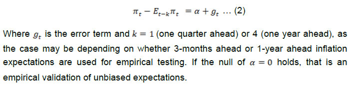 (2) The above test of unbiasedness does not help in understanding the dynamics that drive the inflation expectations process. Information gathering is costly as well as time consuming and therefore assuming households to reflect full information in their expectations may not be appropriate. Even with robust information collection and analytical systems in place, inflation projections of central banks and professional forecasters may deviate from the actual inflation trajectory. Moreover, households often revise their expectations taking into account past forecast errors. If permanent and transitory shocks are not assessed correctly - which can happen even when agents are rational – then one sided errors in expectations could be possible. A realistic assessment of rationality, therefore, should focus on: (a) the long-run relationship (if not convergence) between inflation and inflation expectations, and (b) short-run dynamics in terms of what drives convergence to the long-run relationship. While a test of Granger causality could help verify whether inflation expectations entail any causal influence on inflation or vice versa, co-integration analysis can establish the presence of a long-run relationship and the error correction process can enable investigation of how inflation expectations adjust over time to rational outcomes - or realised inflation (Berk and Hebbink, 2010; Gerberding, 2009). Once co-integration between expected inflation and inflation is established, at least one of the following two error correcting terms must be statistically significant and correctly signed. 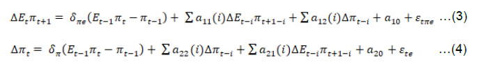 If only the first error correction term matters, then inflation expectations converge to or adjust towards actual inflation. This would suggest that inflation is not influenced by inflation expectations, contrary to NKPC dynamics. However, that could corroborate expectations converging to a rational outcome, as current expectations can be based only the most recently available actual information. If only the second error correction term matters, then inflation converges to inflation expectations, validating the NKPC dynamics. Identifying the nature of inflation expectations is another important aspect of the expectation formation process. Broadly, expectations could be either forward looking, backward looking or naïve (i.e., inability to judge available information, or lack of seriousness while responding to questions in surveys). An unconstrained regression of the following form could help identify the relative role of these three forms of expectations (Sharma and Bicchal, 2018).  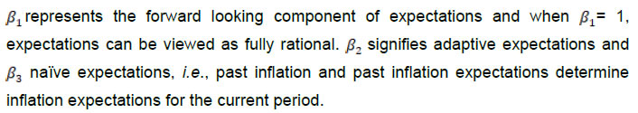 The above mentioned tests are applied to data on CPI inflation and inflation expectations of households for India. The RBI survey of inflation expectations of households, conducted since 20053 on a quarterly basis, collects quantitative and qualitative information on inflation expectations, but the median/mean quantitative value is commonly used to assess how expectations behave relative to underlying CPI inflation. Quarterly information on 3-months ahead and 1-year ahead inflation expectations provide reasonable time series data (Q1:2008 to Q3:2018) to test the above specifications. As the survey data relate to major cities in India, for comparison purpose CPI-urban inflation (new series, for which data are available since 2012) as well as CPI-IW (for which longer time series data are available) have been used. Augmented Dickey-Fuller (ADF) and Phillips-Perron (PP) test results indicate that the variables of interest are I(1) and first difference stationary (Table 1). 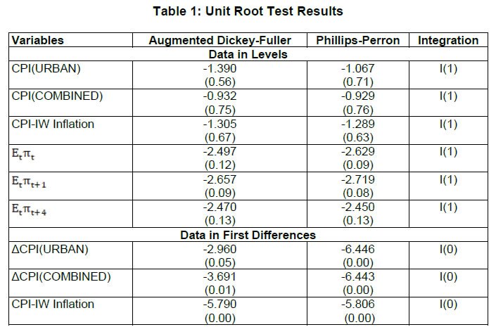 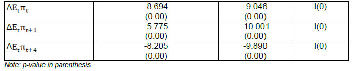 Equation 1 estimates for Indian data relate to three measures of inflation (CPI-C, CPI-Urban and CPI-IW) and two median measures of inflation expectations of households (3-months ahead and 1-year ahead). Inflation data are in terms of quarterly averages because data on inflation expectations are available on a quarterly basis. Correlation coefficients indicate co-movement between inflation and inflation expectations for different lags/leads (Annex Table 1a and 1b). Evolution of both variables over time also suggest likely presence of some cause and effect relationship between them (Annex Chart 1). The joint hypothesis of α = 0 and β = 1 is rejected (as per p-values of Wald test with Newey-West corrected standard errors), suggesting that inflation expectations are not an unbiased predictors of inflation in India (Table 2). 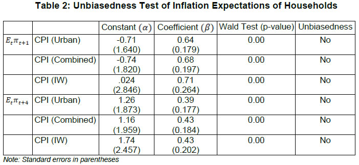 An alternative test of unbiasedness following Equation 2, i.e., α = 0 (as per p-values of t-test with Newey-West corrected standard errors) also suggests that inflation expectations do not work as unbiased predictor of inflation in India (Table 3). Validation of the hypothesis that the mean forecast error is not very different from zero, and given the relative superiority of this test compared with equation 1 (as explained by Holden and Peel, 1990) requires further robustness tests through a deeper analysis of inflation expectations dynamics. | Table 3: Alternative Test of Unbiasedness | | | CPI Urban | CPI- Combined | CPI IW | | | 1 year Ahead | 3 Month Ahead | 1 year Ahead | 3 Month Ahead | 1 year Ahead | 3 Month Ahead | | t-test (d=0) | 6.20*** | 4.39*** | 5.78*** | 3.97*** | 5.15*** | 3.00*** | | * p < 0.05, ** p < 0.01, *** p < 0.001; t-values in parentheses | 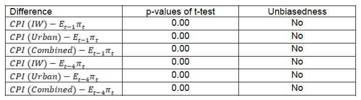 A major reason why any test of rationality or unbiasedness should also explore the underlying dynamics behind the expectation formation process is that rational agents may adjust their forecasts over time to new information and past errors, and even if hard survey-based data show high degree of persistence in errors from expectations (a common test of rejection of rational expectations hypothesis), such errors may not persist in the long-run. Short-term shocks may impact 3-months ahead or 1-year ahead inflation expectations significantly (i.e., disproportionately more than the headline inflation), giving rise to persistence in errors from expectations, which may not persist in the long-run if all agents who provide information through the survey are rational and adjust their expectations taking into account past errors in judgement. The sequential approach to examine underlying dynamics could start with a Granger Causality Test, which is about trying to infer causal relationship between two stochastic variables (inflation and inflation expectations) without imposing any pre-judged theoretical structure. Granger causality test results indicate that inflation expectations do not cause inflation, but instead inflation expectations are influenced by inflation (Table 4). Does this mean inflation expectations do not matter to inflation dynamics in India? The answer to this question is that Granger causality may often be a flawed test of rational expectations – “…If the rational expectation hypothesis is true, it will make Granger-causality tests’ findings contradictory to the real direction of causal relation (Maziarz, 2015).” The argument here is that past and present can influence the future, but future cannot influence current as per the very essence of Granger causality. Notwithstanding this challenge, Granger causality tests are often used in empirical literature on this subject on the ground that expectations about future are formed today, and therefore, expectations that matter to analyse the current state of inflation would have been formed in the past. Survey data may have certain limitations because of which one may not get the expected causal influence of inflation expectations formed in the past on current inflation. 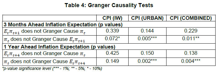 The next step in examining inflation expectations dynamics is to identify whether there is a long-run co-integrating relationship between inflation and inflation expectations, and to assess what the error correction mechanism tells about rationality of expectations. Johansen Trace test results indicate the presence of one co-integrating relationship each between relevant pairs of inflation expectations and inflation, excluding the pair 1-year ahead inflation expectations and CPI-IW inflation (Table 5). Importantly, error correction terms for all relevant pairs (of inflation expectations and inflation) suggest that inflation expectations adjust to the long-run relationship over time (Table 6). This is a test of rationality because expectations converge to the rational value, which is not known at the time when expectations were formed, as households revise their expectations over time. Thus, even when inflation and inflation expectations deviate from their long-run relationship, eventual reversion to the long-term path is ensured by households as they revise their expectations. | Table 5: Johansen Co-integration (Trace Test) | | | CPI (IW) | CPI (URBAN) | CPI (COMBINED) | | Inflation Expectations One quarter ahead (Trace Statistic) | | H0: None | 17.72** | 19.56** | 16.78** | | H1: At most 1 | 3.57 | 2.42 | 2.07 | | Inflation Expectations One year ahead (Trace Statistic) | | H0: None | 13.02 | 20.12** | 17.69** | | H1: At most 1 | 3.27 | 2.35 | 2.20 | | ***, **, * denote significance at the 1, 5, or 10 per cent level. Lag length is as per AIC/SIC criterion. | 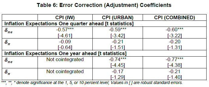 The final step in the process of understanding the inflation expectations dynamics is to test the statistical significance of β1, β2 and β3 in equation 5. While one-year ahead inflation expectations are found to be adaptive, 3-months ahead expectations are both adaptive and naïve. In the short-run, it appears that households repeat expectations of the previous period, and adjust expectations only for new information in actual inflation. This methodology was applied first by Sharma and Bicchal (2018) to Indian data for WPI inflation (for the period Q4: 2006 to Q2: 2015) and the findings were similar to what is reported in this paper for CPI-IW, CPI-C and CPI-Urban. Das (2014) also tested the rationality of household inflation expectations in India using data on WPI and CPI-C for the sample period September 2008 to December 2013 and found that the rationality hypothesis was rejected for CPI-C, if not for WPI. | Table 7: Nature of Inflation Expectations | | | 1-year ahead inflation expectations | 3-months ahead inflation expectations | | | CPI-Urban | CPI-Combined | CPI-IW | CPI-Urban | CPI-Combined | CPI-IW | | β1 (Rational) | -0.288 | -0.287 | 0.00751 | -0.363 | -0.300 | -0.0428 | | β2 (Adaptive) | 0.879*** | 0.884*** | 0.567*** | 0.758* | 0.711* | 0.320 | | β3 (Naive) | 0.243 | 0.273 | 0.246 | 0.476* | 0.460* | 0.491* | | * p<0.05, ** p<0.01, *** p<0.001 | The broad empirical inference that could be drawn from this section is that inflation expectations of households do not influence the process that generates inflation. Notwithstanding some evidence of no systematic errors in judgement (i.e., errors being stationary) and expectations adjusting to the rational outcome through a self-learning process, the expectation formation process is found to be either adaptive or naive. While the estimated error correction results are contrary to the NKPC dynamics, in the next section the statistical significance of inflation expectations in NKPC is tested directly. III: Household Inflation Expectations in the Phillips Curve In the theoretical and empirical literature the treatment of inflation expectations in a Philips Curve framework to study inflation dynamics has changed significantly over time (Gordon, 2013). All broad approaches - the expectations augmented Philips curve, the new Keynesian Philips Curve (NKPC) and the hybrid versions of NKPC – however emphasise that inflation expectations can influence current inflation. In the Gordon triangle approach, inertia, demand and supply are the three key determinants of inflation. As per this approach, past inflation reflects generalised inflation inertia; the role of supply shocks (which could shift the short-run Philips curve) is explicitly recognised; and, output-gap can be used as a convenient proxy of demand conditions. The key point to note in this approach is that when past inflation influences current inflation, it reflects generalised backward looking inertia – arising from either explicit contracts dampening the speed of changes in prices and wages, or input price changes possibly taking longer time to transmit through the supply chain to final prices - rather than backward looking inflation expectations. In NKPC, however, forward looking inflation expectations that respond rationally to policy changes play a key role in influencing inflation. Thus, unlike the Gordon approach, this approach does not recognise any role of inertia or supply shocks, the latter usually getting suppressed in the error term (Equation 6).  As NKPC does not fit real life data well, hybrid versions of NKPC (Gali and Gertlar, 1999) are commonly used in practice (Equation 7)4.  Unlike the emphasis of NKPC on model consistent rational expectations, hybrid expectations are backward looking as well as forward looking, with the relative size of each (when αf and αb are constrained to add up to one, or even otherwise) being a country specific empirical issue. Supply side shocks (Zt) are explicitly recognised as plausible determinants of inflation. et is the serially uncorrelated error term. Recent empirical research for the US suggests that: (a) the role of economic slack (or unemployment gap/output-gap) as a determinant of inflation has weakened significantly (i.e., the slope of the Phillips curve is close to zero); (b) the coefficient of inflation persistence (or backward looking expectations, and in some sense, unanticipated change in inflation) has declined over time; and, (c) the importance of forward looking inflation expectations as a determinant of inflation has increased over time, which highlights the significance of sustained emphasis of monetary policy on anchoring inflation expectations (Jorda et al, 2019) While using survey-based measures of inflation expectations as proxies of forward looking expectations in the above specifications, one needs to recognise that if household expectations are not rational (as found empirically in section II) then such data cannot be used in NKPC, but in hybrid versions of NKPC, survey-based data on expectations may actually work well. In Poland, empirical estimates suggested that survey-based measures of inflation expectations (of consumers, financial market participants, and business enterprises) perform better than model-consistent rational expectations in forecasting inflation (Łyziak, 2010). While several empirical studies on India validate the significance of Phillips curve to explain variations in inflation - notwithstanding differences in the specification of the Phillips curve or in the choice of inflation variable (i.e., WPI, CPI-IW or CPI-C) - we add a new dimension to this research by applying household inflation expectations as a proxy of forward looking expectations for testing the performance of the Phillips Curve in explaining inflation dynamics in India (for a review of empirical studies on India, refer to Behera et al, 2017)5. Using consensus forecast data in NKPC framework (augmented with imported inflation, i.e., international commodity prices) Guimaraes and Papi (2016) found both forward looking and backward looking components of expectations as key determinants of CPI inflation in India, with their respective weights coming close to half. At higher inflation levels, greater inertia (or backward looking expectations) suggested higher sacrifice ratio. Importantly, commodity prices turned out to exert influence on inflation over and above what may be already captured in inflation expectations. Patra et al (2014) tested alternative specifications to establish the relevance of backward looking nature of Phillips curve for India to WPI inflation dynamics, and argued that inflation persistence may have four components, including inflation expectations measured by one period ahead inflation. Given the challenge of measuring inflation expectations, instead of any survey-based data, they used one period ahead actual inflation, and their estimated coefficient at 0.6 was close to the value of the coefficient of intrinsic persistence (or backward looking inflation). Patra and Ray (2010) extracted model based inflation expectations to study what factors influence expectations and concluded that past inflation, food and fuel shocks, output gap and real interest rate can explain variations in inflation expectations. Model consistent rational expectations are incorporated in the framework used by (Benes et al, 2016), under which the expectation formation process is endogenous to monetary policy credibility (i.e., expectations are more backward looking when the credibility is low). Examining Phillips curve relationship at the state level, Behera et al (2017) also confirmed the significance of Phillips curve to explain inflation dynamics in India, but they assumed expectations to be adaptive in all specifications of the Philips curve. Das (2014), using lead WPI inflation as the proxy of forward looking expectations over the sample period Q2:1996 to Q4:2013, and imposing the restriction that the sum of the coefficients for forward looking and backward looking expectations is equal to one, concluded that the coefficient of backward looking expectations generally dominated forward looking expectations, implying high degree of inflation persistence and resultant lagged impact of monetary policy on inflation. Given the available empirical support for the relevance of Phillips curve to India, we attempt to examine the explanatory power of household inflation expectations in explaining variations in CPI-C and CPI-Urban inflation in hybrid versions of the Phillips curve. Since expectations are measured directly through surveys, ordinary least squares (OLS) estimates are used. Moreover, rationality is not imposed a priori, and accordingly a constant is added to all regression equations. Output-gap measures are based on deviations of quarterly GDP from HP filter based trend GDP. When only 3-months ahead inflation expectations and output gap are used as the determinants of inflation, in all five equations (for CPI-C, CPI-Urban, CPI-IW, CPI-C non-food non-fuel, and CPI-Urban non-food non fuel) household inflation expectations emerge statistically significant (Table 8). Output-gap (four quarters lagged) coefficient appears statistically significant for all measures of inflation, excluding CPI-IW. When oil price shock is included in the modified version of the Phillips curve, that does not help improve the explanatory power of the model (Table 9). This would suggest that oil price shocks may not have additional explanatory power beyond what is already captured in households’ inflation expectations. Importantly, the overall explanatory powers of NKPC models with household inflation expectations do not improve relative to similar models with backward looking inflation expectations (Annex Table 2). When both backward looking expectations (inflation with one period lag) and forward looking household expectations were used together in Phillips curve equations (constraining the two coefficients to add up to one, or without imposing any such constraint), individual coefficients appear either very high or low (relative to models with either only backward looking expectations or forward looking expectations), with one of them turning out to be statistically insignificant in most cases (Annex Table 3). Only for CPI-Urban inflation, both past inflation and household inflation expectations are found to be statistically significant, but the output-gap coefficient is not statistically significant in such specifications. Similar results are obtained when 1-year ahead inflation expectations are used (Table 10 and 11). In this section, the aim is to test whether household inflation expectations matter to explain inflation dynamics in a Phillips curve framework in India, rather than to capture the impact of all plausible determinants of inflation. Given that household inflation expectations are adaptive, and also that there is high degree of correlation between past inflation and current inflation expectations (as per Annex Table 1), what this section finds is that household inflation expectations in the Phillips curve – even if they are not fully rational (as discussed in Section II) - help explain inflation dynamics, though only when substituted for backward looking expectations in the in the Phillips curve. Table 8: Phillips Curve without Oil Price Shock
(1-Quarter ahead Inflation Expectations) | | | (1) | (2) | (3) | (4) | (5) | | | CPI Urban | CPI Combined | Core urban | Core combined | CPI (Industrial Workers) | | Three Months ahead Inflation Expectations | 0.798*** | 0.828*** | 0.429*** | 0.401*** | 0.899*** | | | (0.139) | (0.122) | (0.0811) | (0.0636) | (0.172) | | Output Gap (-4) | 0.484* | 0.472** | 0.385** | 0.326** | 0.481 | | | (0.177) | (0.153) | (0.114) | (0.0900) | (0.239) | | Constant | -2.507 | -2.434* | 0.969 | 1.528* | -3.011 | | | (1.256) | (1.147) | (0.789) | (0.604) | (1.629) | | Observations | 22 | 22 | 22 | 22 | 22 | | Adjusted R2 | 0.705 | 0.761 | 0.603 | 0.702 | 0.619 | | ADF test of errors (p-values) | 0.01 | 0.01 | 0.03 | 0.01 | 0.02 | | Note: Standard errors in parentheses. * p < 0.05, ** p < 0.01, *** p < 0.001 |
Table 9: Phillips Curve with Oil Price Shock
(1- Quarter ahead Inflation Expectations) | | | (1) | (2) | (3) | (4) | (5) | | | CPI Urban | CPI Combined | Core urban | Core combined | CPI (Industrial Workers) | | Three Months ahead Inflation Expectations | 0.779*** | 0.816*** | 0.388*** | 0.371*** | 0.936*** | | | (0.135) | (0.121) | (0.0725) | (0.0568) | (0.178) | | Output Gap (- 4) | 0.470* | 0.463** | 0.354** | 0.304** | 0.509 | | | (0.182) | (0.157) | (0.108) | (0.0869) | (0.259) | | Oil Price Shock | 0.0183 | 0.0120 | 0.0402 | 0.0289 | -0.0361 | | | (0.0257) | (0.0220) | (0.0212) | (0.0138) | (0.0303) | | Constant | -2.312 | -2.307 | 1.396 | 1.834** | -3.394 | | | (1.210) | (1.121) | (0.714) | (0.540) | (1.650) | | Observations | 22 | 22 | 22 | 22 | 22 | | Adjusted R2 | 0.694 | 0.750 | 0.648 | 0.733 | 0.613 | | ADF tests errors (p-values) | 0.01 | 0.01 | 0.01 | 0.01 | 0.02 | | Note: Standard errors in parentheses. * p < 0.05, ** p < 0.01, *** p < 0.001 |
Table 10: Phillips Curve without Oil Price Shock
(1-Year ahead Inflation Expectations) | | | (1) | (2) | (3) | (4) | (5) | | | CPI Urban | CPI Combined | Core urban | Core combined | CPI (Industrial Workers) | | One Year Ahead Inflation Expectations | 0.702*** | 0.727*** | 0.388*** | 0.360*** | 0.760*** | | | (0.128) | (0.113) | (0.0777) | (0.0607) | (0.159) | | Output Gap (-4) | 0.394 | 0.379* | 0.337* | 0.281* | 0.378 | | | (0.197) | (0.173) | (0.123) | (0.0998) | (0.265) | | Constant | -2.344 | -2.249 | 0.938 | 1.530* | -2.492 | | | (1.294) | (1.175) | (0.823) | (0.621) | (1.707) | | Observations | 22 | 22 | 22 | 22 | 22 | | Adjusted R2 | 0.692 | 0.743 | 0.624 | 0.716 | 0.557 | | ADF test of errors (p-values) | 0.01 | 0.01 | 0.02 | 0.01 | 0.02 | | Note: Standard errors in parentheses. * p < 0.05, ** p < 0.01, *** p < 0.001 |
Table 11: Phillips Curve with Oil Price Shock
(1-Year ahead Inflation Expectations) | | | (1) | (2) | (3) | (4) | (5) | | | CPI Urban | CPI Combined | Core urban | Core combined | CPI (Industrial Workers) | | One Year ahead Inflation Expectations | 0.688*** | 0.721*** | 0.359*** | 0.341*** | 0.806*** | | | (0.137) | (0.123) | (0.0738) | (0.0557) | (0.183) | | Output Gap(-1) | 0.0216 | 0.0252 | 0.144 | 0.149 | 0.156 | | | (0.317) | (0.270) | (0.171) | (0.130) | (0.357) | | Output Gap (-4) | 0.382 | 0.371 | 0.297* | 0.247* | 0.386 | | | (0.203) | (0.180) | (0.116) | (0.0932) | (0.285) | | Oil Price Shock | 0.0139 | 0.00732 | 0.0335 | 0.0224 | -0.0427 | | | (0.0316) | (0.0269) | (0.0225) | (0.0146) | (0.0393) | | Constant | -2.190 | -2.169 | 1.302 | 1.769** | -2.986 | | | (1.350) | (1.252) | (0.797) | (0.576) | (1.912) | | Observations | 22 | 22 | 22 | 22 | 22 | | Adjusted R2 | 0.659 | 0.714 | 0.656 | 0.748 | 0.528 | | ADF Test of Errors (p-values) | 0.01 | 0.01 | 0.01 | 0.01 | 0.01 | | Note: Standard errors in parentheses. * p < 0.05, ** p < 0.01, *** p < 0.001 | IV: Inflation Expectations and Wage Dynamics One of the major arguments on the need for monetary policy to anchor inflation expectations is that the risk of a wage-price spiral can be averted. Information on household inflation expectations collected through surveys may not fully satisfy the rational expectations hypothesis, but may still contain useful information to help assess how they influence current prices by impacting wage and price setting behaviour of economic agents. In the labour market, inflation expectations of both employers (firms) and employees may determine nominal wage increases. However, given that acquiring new information could be costly, one would expect firms to be more forward looking than employees6. If inflation expectations of employees and employers diverge, then transmission of the former to wages may depend on the degree of unionisation, or bargaining power of labour. In countries that face uncertainty about availability of data on unemployment, wage growth could often be used as an early warning labour market indicator of inflation. Wage growth, however, may reflect the impact of a combination of factors – inflation expectations, slack in the labour market and labour productivity - and the transmission of inflation expectations to inflation may depend on how the latter two factors may be evolving. Moreover, in the presence of large scale involuntary part time employment or temporary contract labourers, transmission of inflation expectations could get dulled. Since the global financial crisis, subdued wage pressures and declining share of labour in total income has complicated assessment of risks to inflation from wages. In the US, the impact of tighter labour market conditions on wages has been dampened by decline in trend productivity growth and labour share in income, even as other factors such as automation, offshoring, decline in unionization and globalisation also played their role (Abdih, 2018). In most advanced economies, nominal wage growth has been more sluggish than what is suggested by standard Phillips curve estimates, and structural changes in the bargaining power of labour and competition from foreign workers could explain part of the subdued wage growth (Arsov, 2018). Greater monopsony power of employers (as highly concentrated labour markets depress wages) and weakening bargaining power of workers have impacted wage dynamics, entailing implications for monetary policy (Krueger, 2018). The importance of wage dynamics in inflation analysis is evident from the high share of labour income in total income. In most developed economies, however, labour shares have declined over time (Pekka, 2011). In India, data from Annual Survey of Industries (ASI) indicate that the shares of wages (of workers) and total emoluments (of salaried employees) taken together constitute about 31.7 per cent of net value added (NVA). As against the industrial sector, for the economy as a whole, national income data suggest that labour share (compensation of employees) in net value added (NVA) is about 34 percent (Chart 1A and 1B). This would suggest that wage dynamics should matter to inflation dynamics, from the stand point of both input cost and aggregate demand effects associated with changes in wage growth. 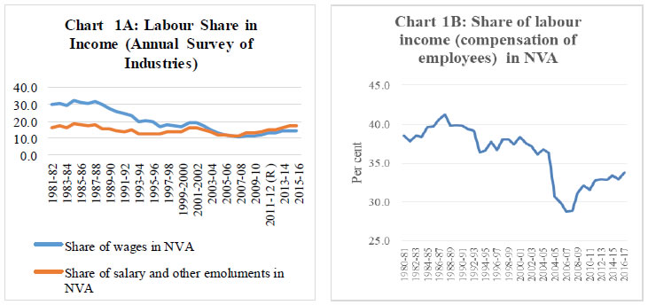 Given that inflation expectations data relate to some major cities, in the absence of data on wages relating to urban areas, data on staff costs (for manufacturing and services) sourced from CMIE are used here. While in the manufacturing sector the share of wages and salaries in total expenses works out to about 6 per cent, in the services sector the comparable share is higher at about 13 per cent7. Strikingly, in the manufacturing sector, per employee costs on wages and salaries have been declining in the recent period, notwithstanding household inflation expectations hovering much above actual inflation, implying the loss of bargaining power of labour. One would expect, therefore, empirical estimates not to validate transmission of inflation expectations to quarterly growth in staff costs. 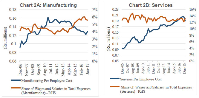 In the absence of data on inflation expectations of households in the rural areas, it is hypothesized that if rural households have similar inflation expectations as in the urban areas (given the high correlation of 0.96 between CPI-urban and CPI-rural inflation for the period January 2012 to December 2018), then inflation expectations of households (one year ahead) can also influence rural wages. Time series data on rural wages suffer from the problem of a statistical break (i.e., the old series is up to October 2013 and the new series is from November 2013, but without a linking factor). Moreover, the classification of labour groups has changed in both series. If one picks common comparable groups from both series, then data on “harvesting” could be used as a proxy for agricultural labourers and data on “masons” could be used as a proxy for non-agricultural labourers. Such data for the period December 2006 to September 2017 plotted in Chart-3 show that there could be some relationship between inflation expectations and rural wages, which could become clearer if estimated empirically8. 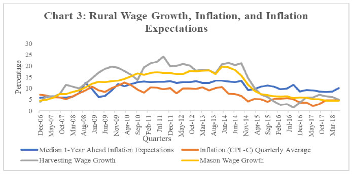 Before starting the empirical exercise, it is hypothesised that the wage-setting behaviour could be influenced by both past inflation (i.e., backward looking) as well as inflation expectations (i.e., forward looking) (Gali, 2011; Blanchard, 1986; Taylor, 1979). Accordingly, the wage setting model used in this paper is: The relevance of both backward looking and forward looking inflation to wage setting behaviour in India (for manufacturing staff costs, services sector staff costs, agricultural wage costs and non-agricultural rural wage costs) is examined here. All variables considered are found to be I(1) (i.e., stationary in first difference), and the estimated results are presented in Table 12. Each equation is estimated twice, i.e., without imposing any restriction on the coefficients of backward looking and forward looking inflation expectations, and then imposing the restriction that these two coefficients add up to one. | Table 12: Inflation Expectations and Wage Growth | | | (1) | (2) | (3) | (4) | | | Harvesting Wage Growth | Mason Wage Growth | Manufacturing per Employee Staff Cost Growth | Services per Employee Staff Cost Growth | | Median One Year Ahead Inflation Expectations | 0.795* | 0.845*** | -1.854* | 0.307 | | | (0.317) | (0.172) | (0.813) | (0.678) | | Inflation (CPI -C) Quarterly Average (t-1) | 0.678 | 0.794** | 1.860** | -0.412 | | | (0.443) | (0.242) | (0.650) | (0.599) | | Dec2013-Sep2014_D | 2.566* | 2.346** | | | | | (1.086) | (0.756) | | | | Post_Dec_2014_D | -9.188*** | -5.431*** | | | | | (2.058) | (1.213) | | | | Constant | 1.804 | -2.399 | 9.039 | 7.926 | | | (3.266) | (1.683) | (7.169) | (7.549) | | Observations | 46 | 46 | 41 | 41 | | Adjusted R2 | 0.75 | 0.88 | 0.20 | 0.01 | | Unit Root Tests of error (p-values) | 0.00 | 0.00 | 0.01 | 0.05 | Wald Test
(Coefficient of median 1-year Inflation Expectations + coefficient of last period CPI–C quarterly average inflation =1) | | F | 1.97 | 13.89 | 2.62 | 2.08 | | Prob > F (p-values) | 0.17 | 0.00 | 0.11 | 0.16 | | Note: Standard errors in parentheses; * p < 0.05, ** p < 0.01, *** p < 0.001. | In the unrestricted formulations of the equations, the coefficients of both lagged inflation and one year ahead inflation expectations of households are correctly signed and statistically significant for non-agricultural rural wages (Table 12). For agricultural rural wages, only forward looking expectations come statistically significant. The explanatory power of inflation expectations in the regression estimates also look high for rural wages. In the restricted versions, F values reject the hypothesis that the two coefficients add up to one for mason wages, which indicates that as per the estimated values of individual coefficients in the equation, the combined impact of backward looking and forward looking expectations on wages could be greater than one. Unlike rural wages, for y-o-y growth in staff costs in the services sector, coefficients of inflation expectations – both past inflation and one year ahead inflation expectations – are not found to be statistically significant. As regards growth in per employee staff costs in manufacturing, the coefficient for one year ahead inflation expectations turns out to be negative and statistically significant, which is consistent with the decline in per employee staff costs in the recent quarters as plotted in Chart 2A One presumes this reflects weaker bargaining power of labour in manufacturing because of similar factors highlighted in the literature for other countries – globalisation and cheaper imports, automation, monopsony power of employers due to concentration of production in large firms, wakening unionisation, etc. To examine whether inflation expectations of more informed households in the sample could alter the findings relating to staff costs, we compared mean values of one year ahead inflation expectations of financial sector employees with other survey respondents, but surprisingly, all categories of respondents seemed to have revealed similar average inflation expectations over time in the past (Annex Chart 2). The second stage of this exercise is to find out whether or not higher wages (influenced by inflation expectations) give rise to higher inflation. This aspect was studied in detail by Kundu (2018) for India, and she found that prices influence wages, rather than wages influencing prices, implying limited risk of a wage-price spiral. These findings were based on estimates that used data on rural wages for the period November 2013 to November 2017. Taking into account the fact that modified Phillips curve approach has already been applied in Section III, in this section inflation is estimated as a function of wage growth (without any output gap variable or other determinants of inflation in the equation) with a view to identifying the presence of any long-run co-integrating relationship between them (using Johansen’s methodology). These estimates use quarterly data for the period December 2006 to June 2018. While modelling, we have used two control dummies: Dec2013-Sep2014_D and Post_Dec_2014_D. The monthly wage series was revised in November 2013. Therefore in wage growth calculation from November 2013 to October 2014 both old and new data are used. To control for this data revision effect we have created a dummy Dec2013-Sep2014_D, which takes the value 1 if the quarter falls in between December 2013 and September 2014, else 0. From December onwards, the wage growth has been calculated using new data only, to control this we have used a dummy Post_Dec_2014_D which is 1 if the quarter is in or after December 2014, else 0. It is observed that agricultural wage growth influences inflation and vice-versa, with the presence of long-run co-integrating vectors (and the statistically significant error correction terms falling within -1 to 0 not only validates the presence of a long term relationship but also indicates short-run adjustments to restore the long-run equilibrium) (Table 13 and 14). For staff costs (both manufacturing and services) Johansen’s co-integrations tests do not provide any evidence of long-run relationship with CPI-C inflation. | Table 13: Vector Error Correction Model for Harvesting Wage Growth | | Short run adjustment equations | | | Δ. Harvesting Wage Growth | Δ. Inflation | | Error Correction Term | -4.09 ×10⁻¹⁴*** | -2.00 × 10⁻¹⁴*** | | Δ.Harvesting Wage Growth | | | | t-1 | 0.019 | 0.188* | | t-2 | -0.072 | -0.190 | | t-3 | 0.257 | 0.142 | | Δ. Inflation | | | | t-1 | -0.170 | 0.057 | | t-2 | -0.412 | -0.199 | | t-3 | -0.048 | -0.194 | | Long run Relationship | | Harvesting Wage Growth=2.818 × CPI Inflation | | *** p<0.01, ** p<0.05, * p<0.1 |
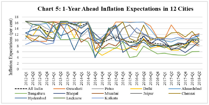
| Table 14: Vector Error Correction Model for Mason Wage Growth | | Short run adjustment equations | | | Δ. Mason Wage Growth | Δ. Inflation | | Error Correction Term | -0.213*** | -0.120*** | | Δ. Mason Wage Growth | | | | t-1 | -0.483*** | -0.449 | | t-2 | 0.157 | 0.079 | | Δ. Inflation | | | | t-1 | 0.092 | -0.122 | | t-2 | -0.145 | -0.199 | | Long run Relationship | | Mason Wage Growth=1.266 × CPI Inflation + 5.329 | | *** p<0.01, ** p<0.05, * p<0.1 | Thus, there is some empirical evidence to support the hypothesis that high inflation expectations of households influence rural wages. Moreover, both agricultural and non-agricultural wages seem to be influenced more by forward looking inflation expectations than past inflation. For rural wages, convergence to long-run steady state also results through adjustments by both wages and inflation, indicating that expectations driven wage pressures could lead to higher CPI-C inflation. This, however, does not stand the test of robustness, because inflation expectations data collected from cities should matter more to growth in staff costs in manufacturing and services activities, where the empirical results do not provide any evidence on inflation expectations induced wage pressures. V: Key Drivers of Household Inflation Expectations When inflation expectations deviate persistently from the inflation target, it becomes important to examine what drives expectations, given the risks highlighted in the previous two sections that high inflation expectations can potentially influence current wage growth and inflation. Past inflation is widely reported in the literature to be a predictor of inflation expectations, as households inherently are subject to “sticky information” problem and often adjust to new information only gradually in a backward looking manner (Ha et al, 2019). Household survey participants may also represent an unknown mix of informed and uninformed consumers9, with the latter assigning disproportionately high weight to frequently purchased items (like food) or what gets publicised widely (like petrol and diesel), which in turn could create a wedge between actual inflation and inflation expectations. The major challenge for inflation management when short-term supply shocks influence inflation expectations is that inflation is not only impacted directly by these shocks but also through second order amplifications. Normally, food and fuel shocks are expected to be transitory and their impact on inflation, though sudden and large, should dissipate over time, allowing space for monetary policy to see through. Moreover, only persistent food and fuel shocks should feed into inflation expectations, posing the challenge of second round amplification, which monetary policy needs to resist. But when transitory shocks also impact inflation expectations, the space for accommodating such shocks may become limited. In countries where credibility of monetary policy is high, not only non-food inflation persistence is low but also transmission of food price shocks to non-food prices is smaller, allowing space to accommodate food shocks. However, in countries with low monetary policy credibility, monetary policy would have to react more forcefully to non-food price shocks because of higher persistence in non-food inflation, and even more forcefully to food price shocks because of the risk of spillover to non-food inflation (Walsh, 2016). When inflation expectations are anchored, the challenge for monetary policy is much less. Anchoring here means relative insensitivity of inflation expectations to incoming data (Bernanke, 2007). In other words, expected inflation should not change because of current inflation increasing in response to a temporary shock. Importantly, changes in inflation may be driven by several non-monetary factors, but monetary policy must anchor inflation expectations for restoring the economy back to stable inflation (Davis, 2012). Survey-based data on inflation expectations usually reflect large heterogeneity in expectations, while empirical literature often focuses on median/ mean values of expectations. This reflects the influence of theoretical macroeconomic models, which assume that people use common information and form expectations rationally, leaving little room for disagreement. Since in real life people tend to differ in many ways, and often widely, in forming their expectations, no single model can possibly help explain how expectations are formed (Mankiw et al, 2003). In India, an analysis of dispersion in individual responses suggested that for 3-months ahead expectations disagreement levels are higher than for 1-year ahead expectations, and there is greater consensus when inflation rises than when inflation declines (Jayaraman et al., 2018). Notwithstanding this challenge, given the importance of inflation expectations to price stability mandate of a central bank which is defined in terms of the headline CPI-C inflation, following the commonly used empirical approach in the literature, this section examines the influence of food and fuel shocks on inflation expectations of households. Available empirical analysis on the subject for India suggests that food and fuel price shocks significantly influence inflation expectations of households. The Report of the Expert Committee to Revise and Strengthen the Monetary Policy Framework (Chairman: Dr. Urjit R Patel) used a panel data framework to examine how food and fuel inflation (as measured in CPI-IW) influence both 3-months and 1-year ahead inflation expectations of households. Empirical evidence on significant influence of food and fuel shocks on inflation expectations was considered as one of the justifications for setting headline inflation as the target for monetary policy. In a Bayesian Vector Auto Regression framework it found that food and fuel shocks had the largest and most persistent impact on inflation expectations. An updated assessment of the same hypothesis (using data for the period September 2008 to December 2014 and specific food and fuel items) yielded somewhat similar results – changes in prices of fruits and vegetables and petrol explain almost 60 per cent of variations in 3-months ahead inflation expectations, while longer-term expectations, as one would expect, were found to be more stable (RBI, 2015). Das et al (2016) found that even after controlling for observed household characterises – such as age group, gender, and employment category – and including lagged inflation in the model, food and energy shocks had significant impact on inflation, though the explanatory power of the model may not increase much. This section uses CPI-Urban and CPI-Combined data over a longer time period to examine the same empirical relationship. In the CPI-C, while data are available for major item groups from 2011, item level data (such as petrol and diesel) are available only since 2014. A panel regression analysis has been used by mapping cities in which inflation expectation surveys are conducted by the RBI to respective CPI-U and CPI-C of states, for the sample period Q1:2012 to Q3:2018. To test how the relationship might have changed over time for CPI-IW, a longer time series data has been used. Inflation in “transportation and communication” (as a proxy for petrol and diesel) and in “fruits and vegetables” are used to study their influence on three months ahead inflation expectations of households. For the panel regression analysis, petrol and diesel is not available separately at the state level, and therefore inflation in miscellaneous group and/or transportation and communication group (which includes petrol and diesel) has been used for analysing oil price shock in the model. Regression results for CPI-IW (sample period Q1:2009-Q3:2018) indicate that a 10 per cent YoY increase in prices of petrol and diesel (i.e., transportation and communication) could increase 3-months ahead inflation expectations by about 2.8 percent. Fruits and vegetables inflation do not show statistically significant impact in the first specification (Table 13). In the second specification, the second lag of fruits and vegetables becomes statistically significant. But, the impact of petrol and diesel (2.2 percentage points) is about seven times higher (compared with 0.3 percentage points for fruits and vegetables) on HH inflation expectations. In the third specification, the second lag of fruits and vegetables and the first leg of transportation and communication are statistically significant. The impact of petrol and diesel (1.6 percentage points) is about four times higher (compared with 0.44 percentage points for fruits and vegetables) on HH inflation expectations. While petrol and diesel explain about 48 per cent of total variation in HH inflation expectations, including fruits and vegetables together they explain about 56 per cent of total variation. | Table 15: Impact of Changes in Food and Fuel Inflation on Inflation Expectations | | | (1) | (2) | (3) | | | 1 year Ahead Inflation Expectation | 1 year Ahead Inflation Expectation | 1 year Ahead Inflation Expectation | | CPI-IW (Transportation and Communication) | 0.280*** | 0.216*** | | | | (0.0528) | (0.0420) | | | CPI – IW (Fruits and Vegetables) | 0.0300 | | | | | (0.0238) | | | | CPI – IW (Fruits and Vegetables) (t-1) | | 0.0207 | 0.0155 | | | | (0.0223) | (0.0227) | | CPI – IW (Fruits and Vegetables) (t-2) | | 0.0312** | 0.0444*** | | | | (0.0149) | (0.0148) | | CPI-IW (Transportation and Communication) (t-1) | | | 0.158* | | | | | (0.0872) | | CPI-IW (Transportation and Communication) (t-2) | | | 0.0605 | | | | | (0.0828) | | Constant | 8.389*** | 8.739*** | 8.701*** | | | (0.589) | (0.409) | (0.416) | | Observations | 39 | 37 | 37 | | Adjusted R2 | 0.48 | 0.53 | 0.56 | | Note: Robust standard errors in parentheses *** p<0.01, ** p<0.05, * p<0.1 | Panel data analysis is particularly suitable while examining inflation expectations of households because of wide cross-section (or inter-city) variations in inflation expectations and also significant intra-city variations in inflation expectations over time (Chart 4 and 5). Appling panel data regression, thus, one could model inflation expectations as a function of not only food and fuel shocks (as captured in CPI-Urban data), but also a state fixed effect (i.e., state specific factor that does not change over time, or, that captures fixed differences in inflation expectations across states), a time fixed effect (or a factor common to all states that changes over time), besides a random error term10. 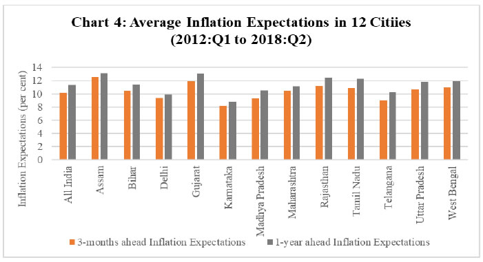
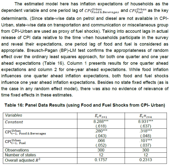 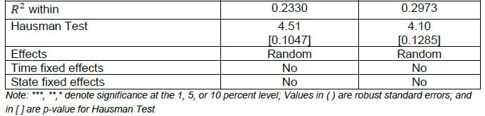 Due to observed persistence in CPI-C inflation and adaptive nature of inflation expectations of households, the baseline static model needs to be augmented with lagged inflation expectations, which in turn would require dynamic panel estimates. A common practice, particularly when cross-section(N) exceeds time period (T) is to use GMM-difference or GMM system estimator proposed by Arellano and Bond (1991), Arellano and Bover (1995), and Blundell and Bond (1998). In this paper, 26 quarterly data points on CPI inflation (since 2012) as against 12 centres (cross-section) for inflation expectations data - or small N and large T - would need to deal with the issue that GMM estimators are likely to produce spurious results (Roodman, 2006)11. Based on Pesaran et al. (1999), we use the following dynamic heterogeneous panel regression incorporated into the error correction model applying the autoregressive distributed lag ARDL (p, q) technique (Fedderke et al., 2003 and Loayza and Ranciere, 2006): 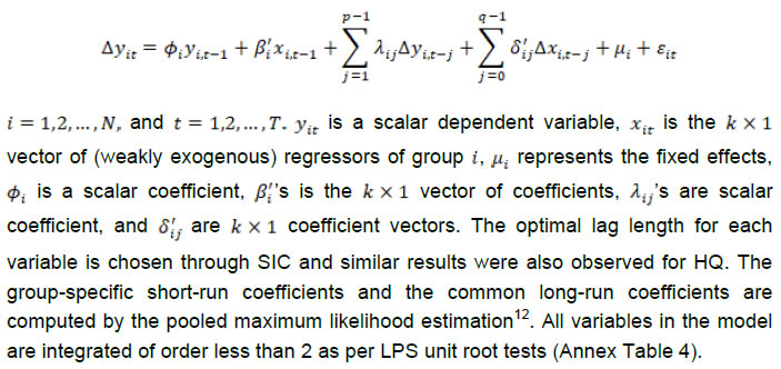 The results are estimated separately with overall food and fuel shocks first in Table-17 (where the miscellaneous group is used as proxy of fuel) and different components of food (cereals, pulses and fruits and vegetables) and fuel (transportation and communication group) in Table 18. While food shocks clearly influence both 3-months ahead and 1-year ahead inflation expectations as per the first specification of the model, each major component of food also appears to be statistically significant in influencing inflation expectations in the second specification. Fuel shocks are not statistically significant in either of the specifications.
VI. Conclusions The usefulness of survey-based information collected by the RBI on inflation expectations of households is examined in this paper from the stand point of their relevance to inflation dynamics and inflation forecasting. For household expectations to satisfy the requirements of both rationality and unbiasedness it is necessary that (a) actual inflation must equal expected inflation on average, and (b) actual inflation must equal expected inflation plus a random forecast error period by period. In other words, while forming expectations, households should not be committing any systematic forecast errors. In practice, it is not necessary that inflation expectations must equal inflation on average, but there must be a long-run (co-integrating) relationship between them and short-run dynamics should ensure convergence to this long-run relationship. From the standpoint of relevance to monetary policy, if inflation expectations drive convergence to the long-term relationship – a rational error learning process that would indicate that inflation is not influenced by inflation expectations. In turn, if inflation drives convergence to the long-run relationship then inflation expectations would have to be viewed as influencing inflation, requiring monetary policy to counter proactively potential risks to the inflation trajectory from inflation expectations. Empirical estimates for India suggest that rationality and unbiasedness hypotheses do not hold for both 3-months ahead and 1-year ahead inflation expectations of households. However, the error correction dynamics obtained from the long-run co-integrating relationship indicate that inflation expectations adjust to the long-run relationship over time. This could be interpreted as an evidence of sensible expectation formation process, if not strictly rational, in the sense that expectations tend to converge to the rational value - which may not be known at the time when expectations were formed - as households revise their expectations over time. Thus, even when inflation and inflation expectations deviate from their long-run relationship, eventual reversion to the long-term path is ensured by households as they revise their expectations. Non-rational nature of expectations do not mean that survey-based information has no utility for explaining inflation dynamics. While rationality is necessary for inflation expectations to be incorporated in a new Keynesian Philips Curve (NKPC), hybrid versions of NKPC often fit actual inflation data better, which also provide a more realistic framework to test the information content of any survey-based measures of inflation expectations. In five different specifications of modified versions of NKPC (for CPI-C, CPI-Urban, CPI-IW, CPI-C non-food non-fuel, and CPI-Urban non-food non-fuel), this paper finds that household expectations emerge as a statistically significant predictor of actual inflation. As household expectations are adaptive, in hybrid NKPC specifications household inflation expectations effectively work more as a substitute of adaptive expectations. Importantly, the explanatory power of NKPC does not improve when household inflation expectations replace past inflation. A realistic assessment of the relationship between inflation expectations and wages – the key channel for transmission of inflation expectations to inflation – often requires information on other key determinants of wages, such as slack in labour market/unemployment rate, labour productivity, trend change in labour share in total income, and other factors such as automation, offshoring, unionization and globalisation. Notwithstanding the potential impact of several factors (some unobserved/difficult to identify), any empirical evidence on inflation expectations influencing wages could be a clear risk to the inflation outlook. For India, growth in staff costs in manufacturing and services activities is used as a proxy of wage growth, given that inflation expectations data relate to cities. Empirical estimates do not provide any robust evidence on transmission of inflation expectations to staff costs. In the absence of inflation expectations data for rural areas, if one assumes that rural areas also have similar inflation expectations as in the cities - given the high correlation between CPI-rural and CPI-urban inflation - then rural agricultural and non-agricultural wages appear to have been influenced by inflation expectations. Assessment based on long-run co-integrating relationship between inflation and rural wages, however, do not yield any evidence of wage growth driving inflation. Despite lack of robust empirical evidence on the role of household inflation expectations in driving inflation in India, given the potential nature of the risks, it is important to understand the factors that drive inflation expectations. Food and fuel shocks tend to influence both 3-months and 1-year ahead inflation expectations of households, together accounting for close to 60 per cent of changes in 3-months ahead inflation expectations in some specifications. A panel regression analysis that recognises the heterogeneity in inflation expectations across cities and the divergent impact of food and fuel shocks on inflation at the state level also establishes the role of food and fuel shocks in driving inflation expectations, but the magnitude of impact is somewhat lower compared with OLS estimates for headline numbers. The space for accommodating temporary food and fuel shocks in the conduct of monetary policy gets increasingly constrained when inflation expectations, instead of remaining anchored to the inflation target, start moving in response to food and fuel shocks, which in turn may amplify inflation pressures by impacting the wage and price stetting behaviour of agents in the economy. The longer such temporary shocks are accommodated by monetary policy, greater the sacrifice of output in the medium-run to restore price stability. But for some possible sampling bias and naïve responses of some households while participating in a survey, household expectations generally should be seen as rational because it may be difficult for even informed agents in the economy to disentangle a transitory shock from a permanent shock, and it is also natural for a household to look back and correct for errors in past expectations over time while setting expectations for the future. Some rational bias in expectations, thus, could be closer to reality compared with text book interpretation of rationality. Moreover, longer-term inflation expectations, say for 5-years ahead or more, could be expected to be much less sensitive to transitory price shocks, and may also impact wage and price setting pattern much more in an economy than 3-months ahead or 1-year ahead expectations. The average time taken to reset wages and prices, based on inflation expectations, could widely differ for different segments of the economy and also for different items in the CPI basket. While retail prices of some perishable may vary every day, that may not be due to changes in inflation expectations. Where inflation expectations matter for wage-price dynamics, longer-term measures of inflation expectations may be more appropriate, and shorter-term expectations like 3-months ahead may actually reflect the influence of more recent past, without much relevance to wage-price setting behaviour of agents in the economy. In India, one may have to also recognise other country specific challenges while studying the behaviour of actual inflation relative to inflation expectations of households. First, quarterly CPI-C and CPI-Urban data are available only since 2012, which statistically limit the scope for robust testing of some of the key empirical hypotheses. Second, this short experience relates to a period of sustained disinflation, preceded by much higher average inflation, which may be still etched in the memory of many households. This sustained disinflation has materialised irrespective of the state of slack in the economy, complicating the assessment of transmission of inflation expectations to wages and prices. Third, inflation expectations data relate to some of the major cities in India, where the share of income spent on certain services, such as education and health, and also transportation and house rent may be much higher than comparable weights in the CPI basket. A more representative mix of respondents in the survey may help in establishing more meaningful empirical relationships between inflation expectations of households and CPI-C and CPI-Urban inflation. The findings of this paper, therefore, may be seen as indicative – based on an attempt to extract as much empirical inferences as one could draw by testing hypotheses that are relevant to understand wage price dynamics in a country – with wide scope for future research as more representative data on inflation expectations and for a longer time period become available.
References Abdih, M. Y., & Danninger, M. S. (2018). Understanding US Wage Dynamics. International Monetary Fund. Arsov, I., & Evans, R. (2018). Wage growth in advanced economies. RBA Bulletin. Behera, H. K., Wahi, G., & Kapur, M. (2017). Phillips Curve Relationship in India: Evidence from State-Level Analysis. Available at SSRN 3050414. Benes, M. J., Clinton, K., George, A., Gupta, P., John, J., Kamenik, O., & Nadhanael, G. V. (2017). Quarterly projection model for India: Key elements and properties. International Monetary Fund. Berk, J. M., & Hebbink, G. (2009). The European consumer and monetary policy. Inflation Expectations, 56, 158. Bernanke, B. (2007). Inflation expectations and inflation forecasting (No. 306). Board of Governors of the Federal Reserve System (US). Blanchard, O. J. (1986). The wage price spiral. The Quarterly Journal of Economics, 101(3), 543-565. Coibion, O., Gorodnichenko, Y., & Kamdar, R. (2018). The formation of expectations, inflation, and the phillips curve. Journal of Economic Literature, 56(4), 1447-91. Das, A. (2014). Role of Inflation Expectation in Estimating a Phillips Curve for India”, RBI (seminar paper). Das, A., Lahiri K. and Zhao, Y. (2016). Asymmetries in Inflation Expectations: A Study Using IESH Quantitative Survey Data.
Available at https://www.iima.ac.in/c/document_library. Davis, J. S. (2012). Inflation expectations have become more anchored over time. Economic Letter, 7. De Brouwer, G., & Ellis, L. (1998). Forward-looking behaviour and credibility: some evidence and implications for policy. Doser, A., Nunes, R. C., Rao, N., & Sheremirov, V. (2017). Inflation expectations and nonlinearities in the Phillips curve. FRB of Boston Working Paper No. 17-11. Available at SSRN: https://ssrn.com/abstract=3072265. Ehrmann, M., Pfajfar, D., & Santoro, E. (2015). Consumers' attitudes and their inflation expectations. FEDS Working Paper No. 2015-015. Available at SSRN: https://ssrn.com/abstract=2595719 or http://dx.doi.org/10.2139/ssrn.2595719. Eruygur, A. (2011). The New Keynesian Phillips Curve: In Search of Improvements for Adaptation to the Turkish Economy. Ekonomik Yaklasim, 22(79), 1-20. Fedderke, J., & Shin, Y. (2003). Trade, technology and wage inequality in the South African manufacturing sectors. Fritzer, F., & Rumler, F. (2015). Determinants of inflation perceptions and expectations: an empirical analysis for Austria. Monetary Policy & The Economy Q, 1, 11-26. Galí, J. (2011). The return of the wage Phillips curve. Journal of the European Economic Association, 9(3), 436-461. Gerberding, C. (2009). Household versus expert forecasts of inflation: New evidence from the European survey data. Inflation Expectations (pp. 136-157). Routledge. Ghosh, T., Sahu, S., & Chattopadhyay, S. (2017). Households' inflation expectations in India: Role of economic policy uncertainty and global financial uncertainty spill-over (No. 2017-007). Indira Gandhi Institute of Development Research, Mumbai, India. Gordon, R. J. (2011). The history of the Phillips curve: Consensus and bifurcation. Economica, 78(309), 10-50. Guimaraes, R. F., & Papi, L. (2016). Inflation Dynamics in India: What Can We Learn from Phillips Curves? Taming Indian Inflation, 1. Gumata, N., & Ndou, E. (2017). The Inflation–Wage Spiral, Inflation Expectations and Monetary Policy. Labour Market and Fiscal Policy Adjustments to Shocks (pp. 373-385). Palgrave Macmillan, Cham. Ha, J., Kose, A., & Ohnsorge, F. (2019). Inflation in Emerging and Developing Economies. Washington, DC: World Bank. Hess, G. D., & Schweitzer, M. E. (2000). Does wage inflation cause price inflation? FRB of Cleveland Policy Discussion Paper, (1). Hubert, P. & Mirza, H. (2018). The Role of Forward and Backward-Looking Information for Inflation Expectations Formation. European Central Bank. IMF (2017). Recent Wage Dynamics in Advanced Economies: Drivers and Implications. World Economic Outlook, Chapter 2, October. IMF (2018).Challenges for Monetary Policy in Emerging Economies as Global Financial Conditions Normalize. World Economic Outlook. October. Jayaraman, A. R., Shaw, P. & Singh, D. P. (2018). Inflation Expectations Survey of Households: 2017-18. RBI Bulletin, October. Jorda, O., Marti, C., Nechio, F., & Tallman, E. (2019). Inflation: Stress-Testing the Phillips Curve. FRBSF Economic Letter, 05. Kapur, M., & Patra, M. D. (2000). The price of low inflation. Reserve Bank of India Occasional Papers, 21(2), 191-233. Kapur, M. (2013). Revisiting the Phillips curve for India and inflation forecasting. Journal of Asian Economics, 25, 17-27. Krueger, A. B. (2018). Reflections on Dwindling Worker Bargaining Power and Monetary Policy. In Luncheon Address at the Jackson Hole Economic Symposium. Kundu, S. (2018). Rural Wage Dynamics in India: What Role does Inflation Play? Reserve Bank of India Working Papers, WPS (DEPR): 03/2018. Loayza, N., & Ranciere, R. (2006). Financial development, financial fragility, and growth. Journal of Money, Credit and Banking, 38(4), 1051-1076. Lyziak, T. (2016). Do inflation expectations matter in a stylised New Keynesian model? The case of Poland. The Case of Poland (February 24, 2016). National Bank of Poland Working Paper, (234). Mankiw, N. G., Reis, R., & Wolfers, J. (2003). Disagreement about inflation expectations. NBER Macroeconomics Annual, 18, 209-248. Maziarz, M. (2015). A review of the Granger-causality fallacy. The journal of philosophical economics: Reflections on Economic and Social Issues, 8(2), 86-105. Meyer, B. (2011). Wages, Expectations and Prospects for Inflation. Economic Trends, 05.31.11, Federal Reserve Bank of Cleveland. Miyajima, K., & Yetman, J. (2018). Assessing inflation expectations anchoring for heterogeneous agents: analysts, businesses and trade unions. BIS Working Paper No. 759. Available at SSRN: https://ssrn.com/abstract=3302315 Patra, M. D., Khundrakpam, J. K., & George, A. T. (2014, August). Post-Global Crisis Inflation Dynamics in India: What has Changed? India Policy Forum (Vol. 10, No. 1, pp. 117-203). National Council of Applied Economic Research. Patra, M. D., & Kapur, M. (2012). A monetary policy model for India. Macroeconomics and Finance in Emerging Market Economies, 5(1), 18-41. Patra, M. D., & Ray, P. (2010). Inflation expectations and monetary policy in India: An empirical exploration (No. 10-84). International Monetary Fund. Pesaran, M. H., Shin, Y., & Smith, R. P (1999). Pooled mean group estimation of dynamic heterogeneous panels. Journal of the American Statistical Association, 94(446), 621-634. Pesaran, M. H., & Smith, R. (1995). Estimating long-run relationships from dynamic heterogeneous panels. Journal of Econometrics, 68(1), 79-113. Posen, A. (2011). The Soft Tyranny of Inflation Expectations. Bank of England and PIIE. RBI (2015). Monetary Policy Report. April. RBI (2014). Report of the Expert Committee to Revise and Strengthen the Monetary Policy Framework. Roodman, D. (2009). How to do xtabond2: An introduction to difference and system GMM in Stata. The Stata Journal, 9(1), 86-136. Sauramo, P. (2011). The relationship between labour share and unemployment: the role of wage-setting institutions. Labour Institute for Economic Research, Finland. Sharma, N. K., & Bicchal, M. (2018). The properties of inflation expectations: Evidence for India. Economia, 19(1), 74-89. Sinclair, P. (2010). Inflation Expectations. Routledge International Studies in Money and Banking. Taylor, J. B. (1979). Staggered wage setting in a macro model. The American Economic Review, 69(2), 108-113. Taylor, J. B. (1982). The Role of Expectations in the Choice of Monetary Policy. NBER Working Paper No. 1044. Visco, I. (2014). Price expectations in rising inflation (Vol. 152). Elsevier. Walsh, J. P. (2016). Reconsidering the Role of Food Prices in Inflation. Taming Indian Inflation.
| Annex Table 1A: Phillips Curve without Oil Price Shock (Adaptive expectations) | | | (1) | (2) | (3) | (4) | (5) | | | CPI Urban | CPI Combined | Core urban | Core combined | CPI (Industrial Workers) | | CPI Urban (-1) | 0.852*** | | | | | | | (0.114) | | | | | | CPI Combined (-1) | | 0.840*** | | | | | | | (0.114) | | | | | Core urban(-1) | | | 0.815*** | | | | | | | (0.106) | | | | Core combined(-1) | | | | 0.793*** | | | | | | | (0.0953) | | | CPI (Industrial Workers)(-1) | | | | | 0.853*** | | | | | | | (0.0958) | | OUTPUT_GAP(-4) | 0.0265 | 0.00541 | 0.0445 | 0.0228 | 0.0516 | | | (0.199) | (0.173) | (0.0989) | (0.0795) | (0.217) | | Constant | 0.641 | 0.742 | 0.895 | 1.051 | 0.641 | | | (0.628) | (0.671) | (0.532) | (0.527) | (0.613) | | Observations | 22 | 22 | 22 | 22 | 22 | | Adjusted R2 | 0.779 | 0.761 | 0.816 | 0.817 | 0.766 | | ADF tests of errors (p-values) | 0.00 | 0.00 | 0.00 | 0.00 | 0.00 | | Note: Standard errors are in parentheses. * p < 0.05, ** p < 0.01, *** p < 0.001. |
| Annex Table 1B: Phillips Curve with Oil Price Shock (Adaptive expectations) | | | (1) | (2) | (3) | (4) | (5) | | | CPI Urban | CPI Combined | Core urban | Core combined | CPI (Industrial Workers) | | CPI Urban(-1) | 0.827*** | | | | | | | (0.101) | | | | | | OUTPUT_GAP (-4) | 0.0116 | -0.0103 | 0.0340 | 0.0123 | 0.0451 | | | (0.185) | (0.160) | (0.0764) | (0.0602) | (0.218) | | Oil Price Shock | 0.0417 | 0.0418 | 0.0462*** | 0.0392*** | 0.0130 | | | (0.0265) | (0.0329) | (0.00954) | (0.00872) | (0.0334) | | CPI Combined(-1) | | 0.818*** | | | | | | | (0.103) | | | | | Core urban (-1) | | | 0.766*** | | | | | | | (0.0789) | | | | Core combined (-1) | | | | 0.752*** | | | | | | | (0.0677) | | | CPI (Industrial Workers)(-1) | | | | | 0.850*** | | | | | | | (0.0945) | | Constant | 0.792 | 0.888 | 1.172* | 1.295** | 0.663 | | | (0.574) | (0.632) | (0.417) | (0.394) | (0.608) | | Observations | 22 | 22 | 22 | 22 | 22 | | Adjusted R2 | 0.796 | 0.777 | 0.898 | 0.899 | 0.755 | | ADF tests of errors (p-values) | 0.00 | 0.00 | 0.00 | 0.00 | 0.00 | | Note: Standard errors in parentheses. * p < 0.05, ** p < 0.01, *** p < 0.001 |
Annex Table 3A: Phillips Curve Estimates with the Restriction that αf + αb =1
(One Quarter ahead Inflation Expectations) | | | (1) | (2) | (3) | (4) | (5) | | | CPI Urban Inflation | CPI Combined Inflation | Urban Core Inflation | CPI Combined Core Inflation | CPI (Industrial Workers) Inflation | | Three Months Ahead Inflation Expectations | 0.465*
| 0.596*
| -0.153
| -0.152
| 0.389 | | | (0.212) | (0.274) | (0.105) | (0.0881) | (0.201) | | CPI Urban (-1) | 0.535* | | | | | | | (0.212) | | | | | | CPI Combined Inflation (-1) | | 0.404 | | | | | | | (0.274) | | | | | CPI Urban Core Inflation(-1) | | | 1.153*** | | | | | | | (0.105) | | | | CPI Combined Core Inflation (-1) | | | | 1.152*** | | | | | | | (0.0881) | | | CPI (Industrial Worker) Inflation (-1) | | | | | 0.611** | | | | | | | (0.201) | | Output Gap (-1) | 0.124 | 0.112 | -0.0499 | -0.0564 | 0.0832 | | | (0.196) | (0.212) | (0.150) | (0.125) | (0.217) | | Output Gap (-2) | 0.384 | 0.297 | -0.160 | -0.191 | 0.190 | | | (0.388) | (0.394) | (0.201) | (0.165) | (0.521) | | Output Gap (-3) | 0.229 | 0.230 | -0.00393 | -0.0418 | 0.118 | | | (0.150) | (0.173) | (0.123) | (0.0971) | (0.186) | | Output Gap (-4) | 0.383 | 0.395 | -0.192 | -0.220 | 0.283 | | | (0.277) | (0.313) | (0.167) | (0.128) | (0.320) | | Oil Price Shock | -0.000792 | -0.00320 | 0.0537** | 0.0508** | -0.0206 | | | (0.0358) | (0.0402) | (0.0170) | (0.0159) | (0.0463) | | Constant | -1.938* | -2.334* | 0.547 | 0.446 | -1.598* | | | (0.857) | (0.994) | (0.416) | (0.323) | (0.722) | | Observations | 22 | 22 | 22 | 22 | 22 | | Note: Standard errors in parentheses. * p < 0.05, ** p < 0.01, *** p < 0.001 |
Annex Table 3B: Phillips Curve Estimates with the Restriction that αf + αb = 1
(One-year ahead Inflation Expectations) | | | (1) | (2) | (3) | (4) | (5) | | | CPI Urban Inflation | CPI Combined Inflation | Urban Core Inflation | CPI Combined Core Inflation | CPI (Industrial Workers) Inflation | | One Year Ahead Inflation Expectation | 0.170 | 0.290 | -0.152* | -0.134 | 0.197 | | | (0.210) | (0.243) | (0.0711) | (0.0637) | (0.139) | | CPI Urban (-1) | 0.830** | | | | | | | (0.210) | | | | | | CPI Combined Inflation (-1) | | 0.710* | | | | | | | (0.243) | | | | | CPI Urban Core Inflation (-1) | | | 1.152*** | | | | | | | (0.0711) | | | | CPI Combined Core Inflation (-1) | | | | 1.134*** | | | | | | | (0.0637) | | | CPI (Industrial Worker) Inflation (-1) | | | | | 0.803*** | | | | | | | (0.139) | | Output Gap (-1) | 0.0470 | -0.0123 | -0.0259 | -0.0273 | 0.000254 | | | (0.217) | (0.229) | (0.152) | (0.123) | (0.233) | | Output Gap (-2) | 0.218 | 0.139 | -0.161 | -0.182 | 0.0760 | | | (0.394) | (0.401) | (0.188) | (0.155) | (0.519) | | Output Gap (-3) | 0.138 | 0.114 | 0.0329 | -0.00402 | 0.0463 | | | (0.145) | (0.162) | (0.121) | (0.0886) | (0.181) | | Output Gap (-4) | 0.130 | 0.131 | -0.182 | -0.198 | 0.120 | | | (0.272) | (0.256) | (0.146) | (0.119) | (0.272) | | Oil Price Shock | 0.0154 | 0.0138 | 0.0552** | 0.0505** | -0.00677 | | | (0.0377) | (0.0431) | (0.0158) | (0.0147) | (0.0441) | | Constant | -0.974 | -1.597 | 0.737 | 0.544 | -1.192 | | | (1.072) | (1.180) | (0.352) | (0.320) | (0.742) | | Observations | 22 | 22 | 22 | 22 | 22 | | Note: Standard errors in parentheses; * p < 0.05, ** p < 0.01, *** p < 0.001 |
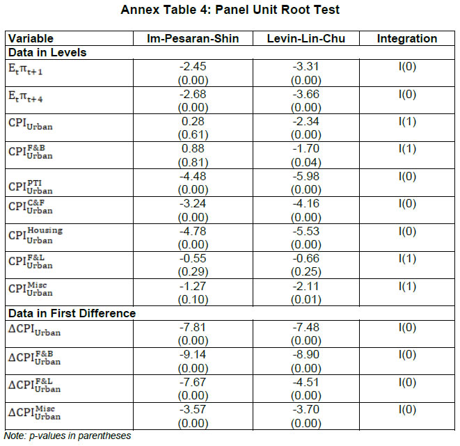 |