Press Release RBI Working Paper Series No. 04
Economic Activity and its Determinants: A Panel Analysis of Indian States @Garima Wahi and Muneesh Kapur Abstract 1This paper assesses the impact of both monetary and fiscal policy along with other macroeconomic determinants on economic activity using state-level Indian data. Since economic activity can vary across states due to local factors and state government policies, a state-level empirical analysis, by providing more variability in both the dependent variable and the potential explanatory variables, can help better identify the underlying economic relationships. The empirical analysis confirms the role for a countercyclical monetary policy in stabilising economic activity. Bank credit expansion supports economic activity, suggesting the operation of credit channel of transmission in addition to the interest rate channel. Public investment is found to crowd-in economic activity, while other fiscal spending crowds out economic activity. JEL classification: E23, E43, E52, E58, E62, E63, F32, F41 Keywords: bank credit, exchange rate, fiscal policy, India, IS curve, monetary policy, monetary transmission, output I. Introduction Output dynamics at the business cycle frequency are impacted by the stance of monetary and fiscal policies, exchange rate movements and global demand conditions – these macroeconomic determinants and their relative importance in the Indian context are the focus of this paper. From the monetary policy transmission perspective, modulations in policy interest rate impact inflation through their impact on domestic demand and output. There exists an extensive research pertaining to the second part of the transmission process – from demand conditions to inflation in a Phillips curve framework - both for India and globally (Behera, Wahi and Kapur, 2017). The empirical literature focusing on the first stage of the transmission – from interest rates to demand and output in an IS curve framework – is, however, relatively scarce (Coeure, 2017). While several papers have assessed both the legs of the transmission in an integrated manner (for example, Patra and Kapur, 2012), all the existing studies on the IS curve2 for India are based on national level data. There is, however, some evidence that national level data may not be able to identify the pure IS curve adequately, leading to the “IS curve puzzle” phenomenon (Goodhart and Hofmann, 2005).3 The “IS curve puzzle”, if true, would imply that monetary policy is ineffective in its ability to contain demand pressures and inflation in the economy. The observed “IS curve puzzle” in some empirical studies could be due to the simultaneity bias4 in the estimation or due to omitted variables (such as long-term interest rates, exchange rate, money supply, asset prices and external demand) that also impact demand. Indeed, in the specifications augmented with property prices (as an indicator of wealth effects), Goodhart and Hofmann (2005) find a negative and significant coefficient on the real interest rate, thus solving the IS puzzle. As regards the endogeneity bias in regressions involving national level data, it can be minimised by recourse to sub-national data. From this paper’s perspective, we may note that keeping national level inflation rate close to its mandated target and national output gap close to zero are the objectives of a central bank. The sub-national demand and output dynamics are, however, not the goals of monetary policy per se. Thus, a study employing state-level data, as is the approach taken in this paper, can address the simultaneity/endogeneity concerns vis-à-vis a study using national level data. Furthermore, by providing more variability in both the output dynamics and the explanatory variables, the sub-national level data can overcome some of the limitations of national data and thus help to better identify the IS curve. Finally, in view of the fiscal stance varying across states and time, the state-wise panel approach can throw some light on the role of these key variables in influencing economic activity in an integrated framework. The approach can also help to understand the impact of alternative instruments of fiscal spending (higher fiscal/revenue deficits vis-à-vis higher capital outlays) on demand and output. While the Indian economy has registered a strong overall growth of around 7 per cent per annum since 1992-93, the regional growth is marked by imbalances and disparity (IMF, 2017; Chakravarty and Dehejia, 2016). In such a milieu, an analysis of sub-national panel dataset can help to identify more precisely the role of the various macroeconomic drivers of growth vis-à-vis the studies relying on national data. Accordingly, this paper estimates pure and augmented IS curve relationships in a panel framework using the Indian state-level data.5 The recourse to state-level data permits us to assess the role of both monetary and fiscal policies on economic activity in an integrated manner, whereas the available IS curve studies have restricted themselves to analysing only the impact of monetary policy on demand. A preliminary look at state-level data shows negative association of output with real interest rate, real exchange rate, and revenue deficit on the one hand, and a positive association with capital outlays on the other hand (Chart 1). In the Indian context, most studies of the IS curve have concentrated on the short-term interest rate as an instrument of monetary policy, without accounting for the fiscal policy impact. In addition to the short-term policy repo rate, this paper explores the role of medium-and long-term interest rates in determining the pace of domestic demand as a robustness test, while recognising that such medium-and long-term rates are not fully under the control of monetary policy. 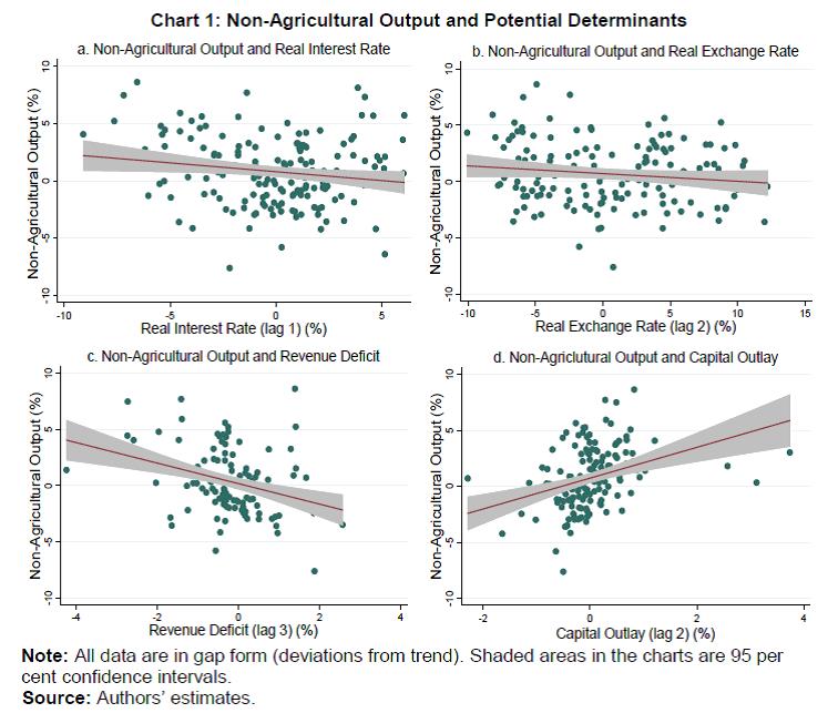 The paper’s empirical analysis confirms, first, the countercyclical role of monetary policy in stabilising aggregate demand: higher interest rates reduce demand and lower interest rate support economic activity. Second, on fiscal policy, higher public investment (capital outlay) is found to provide a boost to non-agricultural output, whereas higher revenue and fiscal deficits crowd-out private sector activity. The crowding out impact of higher revenue deficits on output is found to be more conspicuous in low income states. Unlike some existing studies, we are unable to find any positive effect of higher deficits even in the short-term. Thus, public spending oriented towards productive and capacity enhancing capital outlays, while adhering to prudent deficit targets, can have a positive impact on economic activity. Third, there is evidence in favour of a bank credit channel – the higher the volume of bank credit, the higher the level of output – over and above the interest rate channel of monetary policy. The recent stress in the asset quality of public sector banks and the concomitant slowdown in credit availability from these banks can thus be expected to dampen domestic output. Although the continued strong credit supply from private sector banks and the non-banking financial segment is offsetting some of the slowdown, the ongoing efforts to strengthen asset quality of public sector banks bode well for allocative efficiency and financial stability in the medium term even if there is some short-term pain in the process (RBI, 2018). Finally, the empirical analysis points to the role of external demand as an important driver of domestic demand along with real exchange rate dynamics - the buoyant global demand since 2017 has been positive for the domestic economy, but recent protectionist tendencies and higher crude oil prices, if sustained, can impart headwinds to domestic activity going forward. The remainder of the paper is structured as follows: Section II reviews the existing literature pertaining to the IS curve, with a focus on empirical studies geared towards analysing regional output dynamics. Section III discusses the estimation methodology and the data sources. Section IV presents and analyses key results, with concluding remarks in Section V. II. Literature Review Three main aggregate relationships define the monetary transmission process in the modern new Keynesian model. The first leg of the transmission – the new Keynesian IS curve - relates aggregate demand to ex ante real interest rate and expected demand. The second leg – the new Keynesian Phillips curve – postulates that inflation responds to expected inflation and marginal costs (often proxied by output gap). The third and final leg that completes the model is a monetary policy rule (for example, the Taylor rule) linking the nominal policy rate to deviations of inflation and output from their respective target/potential (Clarida, Gali and Gertler, 1999; Woodford, 2003). The textbook micro-founded New Keynesian model is completely forward-looking: expected inflation determines current inflation and expected output determines current output. The actual output and inflation dynamics, however, are marked by substantial persistence for a variety of reasons such as habit persistence, liquidity constrained households, and menu costs. This has led to hybrid IS and Phillips curves, with lagged output and lagged inflation introduced through ad hoc adjustments in the modelling approach. The empirical evidence, however, seems to favour backward-looking specifications both for the Phillips curve (Rudd and Whelan, 2007) and for the IS curve (Fuhrer and Rudebusch, 2004). In the case of the IS curve, Fuhrer and Rudebusch (op cit) find that (a) the generalized method of moments (GMM) approach to estimating the forward-looking IS curve biases the coefficient on expected output gap towards 0.5, even though the true coefficient may be below/above 0.5, (b) the maximum likelihood estimates indicate that the coefficient on expected output gap is quite often insignificantly different from zero, and (c) the real interest rate has the expected negative and significant effect on output gap only in a backward-looking specification. The panel analysis for 22 OECD countries in Stracca (2010) corroborates Fuhrer and Rudebusch (2004) conclusion: the real interest rate turns out to be either insignificant or wrongly signed in forward-looking specifications. In the New Keynesian model, the IS curve relates output gap to the expected path of short-term interest rates, with no direct role for the medium- and long-term interest rates which are more relevant for spending decisions by both households and firms. For the US, the empirical evidence suggests that the short-term interest rate has a larger influence on aggregate spending through its impact on the entire term structure (Kiley, 2014). In the presence of unconventional monetary policies pursued by the advanced economies since 2008 aimed at softening long-term yields, the short-term interest rate may not be the appropriate measure of financial conditions, especially in times of severe financial crisis. For euro area, the empirical evidence confirms this hypothesis: the coefficient on the real interest rate turns statistically significant when the short-term interest rate is replaced with a measure of the composite bank-based cost of borrowing for non-financial firms (Coeure, 2017). Regional analysis for the US indicates a strong negative correlation between changes in housing prices and changes in the unemployment rate. During the 2008-09 Great Recession, the US counties with larger decreases in house prices experienced larger increases in the unemployment rate, and vice versa during the subsequent expansion of 2010-16 (Dvorkin and Shell, 2016). The state-level estimates of the IS curve in Cooper et al. (2016) indicate that an increase of 100 bps in the real interest rate increases the unemployment rate by about 80 bps after two years – the effect is substantially higher than the national level estimate of around 50 bps. Thus, the monetary policy impact on economic activity may be stronger than suggested by national level estimates; however, it is difficult to generalise this finding in view of the limited number of such studies. Moving to other determinants of economic activity, exchange rate depreciation, even a temporary one, can lead to a durable improvement in profits, investment, and sales of firms that are more financially-constrained and have higher labour shares by boosting their cash flows/retained earnings (Dao et al., 2017). According to the analysis in IMF (2015), real effective depreciation of 10 per cent is associated with a rise in real net exports of, on average, 1.5 per cent of GDP (with substantial cross-country variation of 0.5-3.1 per cent), and with much of the adjustment occurring in the first year. The growth-boosting effect of currency depreciation through the trade channel could, however, get offset, partly or fully, in the presence of sizeable foreign currency borrowings (BIS, 2016). Finally, the role of fiscal policy in promoting economic stabilization continues to be a matter of debate, although there is somewhat more support for it in the aftermath of the 2008-09 Great Recession (Auerbach, 2017). Ramey (2017), however, argues that the most robust aggregate estimates of spending multipliers lie below unity. Moreover, the fiscal multiplier could be lower if the initial level of public debt is high, especially for emerging economies as these have relatively lower debt intolerance levels. Empirical Evidence: India Many studies have examined the relationship between monetary policy and economic activity as a part of the overall monetary transmission mechanism – both in a New Keynesian modelling framework and in VAR framework, although only a few studies have focussed on the IS curve per se. In an augmented IS curve framework, the estimates in Kapur and Behera (2012) indicate that an increase of 100 bps in the nominal policy rate leads to a peak decline of 40 bps (with a lag of 2 quarters) in non-agricultural growth; the impact was found to be somewhat lower when real interest rate was used in lieu of nominal interest rate. Patra, Khundrakpam and Gangadaran (2017) compare the aggregate demand dynamics for the pre-financial crisis period vis-à-vis the post-crisis period and find that the impact of the real policy rate on output has declined, while the importance of external demand seems to have increased in the post-crisis period. According to Salunkhe and Patnaik (2018), the backward-looking IS model fits the data better in comparison with the hybrid model and there is a role for additional variables (real exchange rate, external demand and crude oil prices). An expansionary fiscal policy in the form of a higher revenue deficit can have a short-run positive impact on economic activity, but the effect dissipates/turns negative over time; fiscal multipliers for capital outlays exceed consumption expenditure in the long-run (Jain and Kumar, 2013; Tapsoba, 2013). According to Ganesh-Kumar et al. (2017), fiscal stimulus in boom times leads to crowding out of productive investment; an expansionary fiscal policy during recessionary periods is not always beneficial. As regards the determinants of output in a regional setting, Nachane et al. (2002) in a structural vector autoregression (SVAR) framework find that economic activity in states with a higher share of manufacturing activity in output or with deeper bank penetration is more sensitive to monetary policy shocks. Overall, the available empirical evidence, both for India and cross-country, indicates that higher interest rates and currency appreciation dampen demand. Higher public investment has a more durable impact on output, whereas current government spending has at best a short-run positive impact on demand. However, an integrated approach to assess the role of the various determinants of demand and output in a unified framework is missing. Against this backdrop, we undertake a state-wise panel approach to assess the determinants of output and demand, extending the approach adopted by Behera, Wahi and Kapur (2017) to assess the Phillips curve dynamics in a similar setting. III. Methodology and Data The cross-country literature review on the IS curve in the previous section suggests clear evidence in favour of a backward-looking version.6 Moreover, the IS curve is identified better, when augmented with relevant conditioning variables like exchange rate, credit/monetary aggregates, asset prices, external demand. Furthermore, the stance of the fiscal policy (the overall deficit and its composition) is potentially an important determinant of economic activity. On the relevance of using state-wise data to assess the determinants of output and demand, we may note that, first, the national level data can be seen as an aggregation of economic activity in the various states. If the national level data indicate an acceleration in output growth, it would be a reflection of state-level growth dynamics (with some states recording growth quite close to the national growth rate and others registering growth above or below the all-India growth rate). Second, the analysis in World Bank (2018) suggests that in the aftermath of the 2008 global financial crisis: (i) the economic cycles in the Indian states were similar to those experienced at the national level; (ii) the growth cycles were more pronounced in non-agricultural states (i.e., states with a relatively higher share of manufacturing and services activities in their output) relative to agricultural states. These findings suggest that global factors influence state level output and hence there is a merit in including an indicator of external demand in the regressions. Third, states that export more internationally, and trade more with other states, tend to be richer, and the correlation is stronger between prosperity and international trade (Government of India, 2018). These observations also provide a rationale for inclusion of a variable capturing external demand conditions in the regression analysis. Fourth, the empirical evidence for India as well as cross-country suggests that an expansionary monetary policy leads to higher demand and output at all-India level (for example, Kapur and Behera, 2012); again, such national level impacts would exist only if a monetary expansion boosts demand and output at the regional level. Here, one can analytically think of the Indian states like euro area countries, with a common monetary policy. Finally, the advantage of the state-level panel data, as alluded to earlier, is that it can mitigate the endogeneity issues facing the studies relying on national level data. As the deviations of all-India inflation and output from their target/potential levels are policy objectives, the recourse to state-level data on these variables (which are not policy objectives per se) can address, to a large extent, the endogeneity concerns and the concomitant downward bias to the estimated coefficients highlighted by Goodhart and Hofmann (2005). The agricultural sector continues to be an important component of domestic output and driver of demand in India, and its performance remains dependent, inter alia, on the monsoon progress. While the share of agriculture in the domestic output has been falling over the years, it is still sizeable with a share of 17 per cent in domestic value added (current prices) in 2016-17. Shocks to the monsoon activity can thus, have a substantial impact on domestic demand in the short-run. The agriculture sector’s output is also likely influenced by a host of other policy interventions by the government (such as minimum support prices, procurement operations, interest subventions). In view of these factors, we also model the determinants of non-agricultural output (yn), which is our baseline regression, in addition to overall output (y). Given the dynamic panel, the system generalized method of movements (GMM) approach of Arellano-Bond-Bover is used to estimate the following equations: output (both yn and y) is postulated to depend on its lag, real interest rate (r), world output (wy), real effective exchange rate (reer), real bank credit (bc) and fiscal (fisc) variables (fiscal deficit (fd), or revenue deficit (rd) or capital outlay (co)).7 Data State-wise output is measured by real gross state value added (GSVA) and annual growth rates are used to splice the series across different base years. The state-level output data, the key variable of the study, are available on an annual basis (financial year), and thus all other variables are used at an annual frequency for the estimation. To understand the impact of monetary policy on economic activity, the baseline regressions use the effective policy rate, following Patra and Kapur (2012). As a robustness analysis, the alternative specifications use a range of medium- and long-term interest rates, since such rates have an impact on spending decisions of households and firms. Real effective policy rate in each case is the relevant nominal interest rate less the state-specific CPI inflation rate (based on consumer price indices for industrial workers, CPI-IW). State-wise real effective exchange rates are the all-India 36-currency trade-weighted real effective exchange rate, adjusted by state-wise CPI-IW. Monetary policy impacts activity not only through the interest rate channel, but also through the credit channel, especially in a bank-dominant economy such as India. We initially tested for this channel by including state-wise bank credit (state-wise sanction as well as utilisation of credit). However, both these variants of state-wise bank credit did not yield meaningful results. Borrowers with multiple factories/units across states can borrow in one state and allocate credit to their factories/units across states and the available data may not be able to adequately capture such credit dynamics. In view of this, we use all-India real non-food bank credit (deflated by state-wise CPI-IW) to capture the credit channel. The fiscal impact on economic activity is assessed for alternative indicators of fiscal stance as well as the quality of fiscal spending. We study the impact of variations in key deficit indicators (fiscal deficit, or revenue deficit8) and the quality of spending (capital outlay) – with all the variables taken as a ratio of the respective state-level GVA. Finally, external demand is captured by movements in world output. All the variables in the empirical exercise are used in the gap form, i.e., actual less its Hodrick-Prescott (HP) filtered series (multiplied by 100 to get the gap in percentage terms, as needed).9 Overall, the study covers non-special category states/union territories (UTs) for the period 2007-08 to 2015-16.10 All data used are available in public domain, namely, Reserve Bank of India, Central Statistics Office, Labour Bureau, Directorates of Economics and Statistics of respective states and International Monetary Fund. Summary statistics for key variables are presented in Table 1. Large variation, both within and between, supports the case for panel estimation. | Table 1: Summary Statistics | | (Per cent) | | Variable | | Mean | Standard Deviation | Minimum | Maximum | | Real GDP Growth | overall | 6.8 | 3.1 | -6.3 | 18.7 | | | between | | 0.9 | 5.5 | 8.8 | | | within | | 3.0 | -5.9 | 17.7 | | Real Non-agricultural GDP Growth | overall | 7.6 | 3.5 | -7.2 | 21.3 | | | between | | 1.0 | 5.6 | 9.8 | | | within | | 3.3 | -6.1 | 20.5 | | Real Bank Credit Growth | overall | 7.6 | 4.5 | -1.4 | 17.3 | | | between | | 0.6 | 6.1 | 8.6 | | | within | | 4.5 | -1.3 | 17.4 | | Fiscal Deficit (Per cent to GSVA) | overall | 2.6 | 1.5 | -1.7 | 7.4 | | | between | | 1.1 | 0.7 | 5.2 | | | within | | 1.1 | -0.4 | 6.9 | | Revenue Deficit (Per cent to GSVA) | overall | -0.4 | 2.1 | -9.2 | 5.4 | | | between | | 1.8 | -4.2 | 2.9 | | | within | | 1.2 | -5.4 | 4.2 | | Capital Outlay (Per cent to GSVA) | overall | 2.8 | 2.0 | 0.5 | 13.7 | | | between | | 1.8 | 0.9 | 9.3 | | | within | | 1.0 | -1.7 | 7.1 | | Policy Rate, real | overall | -1.3 | 3.5 | -11.7 | 4.2 | | | between | | 0.6 | -2.7 | -0.2 | | | within | | 3.5 | -11.6 | 5.4 | | Weighted Average Lending Rate, real | overall | 3.5 | 2.8 | -4.5 | 8.5 | | Yield on 1-year Government Security, real | overall | -0.9 | 3.2 | -10.5 | 4.6 | | Yield on 5-year Government Security, real | overall | -0.4 | 2.7 | -8.1 | 5.0 | | Yield on 10-year Government Security, real | overall | -0.3 | 2.7 | -7.8 | 4.9 | | Yield on 1-year Corporate Bond, real | overall | 0.5 | 3.1 | -9.0 | 5.4 | | Yield on 5-year Corporate Bond, real | overall | 0.8 | 2.7 | -6.8 | 5.6 | | Yield on 10-year Corporate Bond, real | overall | 0.9 | 2.6 | -6.4 | 5.6 | | Real Effective Exchange Rate Variation | overall | 1.9 | 6.8 | -13.1 | 17.5 | | World Real GDP Growth | overall | 3.5 | 1.5 | -0.1 | 5.5 | Note: GSVA: Gross State Value Added. Data for all variables are for the period 2007-08 to 2015-16.
Source: Authors’ estimates. | IV. Estimation Results Estimates for Non-agricultural GDP Starting with estimates for non-agricultural output, like some other studies, we do observe the phenomenon of the IS curve puzzle for the pure IS curve, i.e., when the real interest rate is the only explanatory variable (apart from the lagged output gap) (Table 2, column 1). The IS curve puzzle, however, disappears in the specifications augmented with variables capturing external demand, exchange rate, fiscal variables, and bank credit. The key results from our analysis are: first, the absolute value of the real interest rate coefficient almost trebles from (an insignificant) 0.11 in the simple bivariate IS curve (column 1) to 0.31-0.37 in the extended specifications (columns 2 to 7). Thus, simple specifications can be biased downwards and underestimate the impact of monetary policy on demand. The diagnostic tests for all specifications are satisfactory: the over-identifying restrictions and the null of no (second-order) autocorrelation are not rejected at conventional significance levels.11 | Table 2: GMM Estimates of the IS Curve using Non-Agricultural GDP and Real Policy Rate - Lag 2 onwards as instruments | | Explanatory Variables | 1 | 2 | 3 | 4 | 5 | 6 | 7 | | yni,t-1 | 0.43*** | 0.37*** | 0.34*** | 0.30*** | 0.32*** | 0.32*** | 0.26** | | | (0.00) | (0.00) | (0.00) | (0.00) | (0.00) | (0.00) | (0.01) | | pri,t-1 | -0.11 | -0.35*** | -0.37*** | -0.31*** | -0.34*** | -0.36*** | -0.33*** | | | (0.23) | (0.00) | (0.00) | (0.01) | (0.00) | (0.00) | (0.01) | | wyt-1 | | 0.80*** | 0.68*** | 0.59*** | 0.67*** | 0.77*** | 0.60*** | | | | (0.00) | (0.01) | (0.01) | (0.00) | (0.00) | (0.01) | | reeri,t-2 | | -0.12*** | -0.13*** | -0.09* | -0.11** | -0.22*** | -0.19*** | | | | (0.01) | (0.01) | (0.08) | (0.02) | (0.00) | (0.00) | | fdi,t-1 | | | -0.44 | | | | | | | | | (0.24) | | | | | | rdi,t-3 | | | | -0.58*** | | | -0.48*** | | | | | | (0.00) | | | (0.01) | | coi,t-2 | | | | | 0.55* | | | | | | | | | (0.07) | | | | bci,t-1 | | | | | | 0.30** | 0.28** | | | | | | | | (0.03) | (0.04) | | constant | 0.31** | 0.03 | 0.11 | -0.04 | 0.18 | -0.34** | -0.35** | | | (0.03) | (0.79) | (0.27) | (0.75) | (0.18) | (0.02) | (0.01) | | Observations | 168 | 168 | 160 | 160 | 160 | 168 | 160 | | No. of instruments | 71 | 92 | 134 | 134 | 134 | 92 | 134 | | AR(1)-test (p-value) | 0.02 | 0.01 | 0.01 | 0.01 | 0.01 | 0.01 | 0.01 | | AR(2)-test (p-value) | 0.38 | 0.60 | 0.70 | 0.68 | 0.53 | 0.56 | 0.57 | | Sargan test (p-value) | 0.02 | 0.28 | 0.56 | 0.45 | 0.63 | 0.29 | 0.46 | | Hansen Test (p-value) | 1.00 | 1.00 | 1.00 | 1.00 | 1.00 | 1.00 | 1.00 | Notes: Figures in parentheses are p-values.
AR(1) and AR(2) are Arellano–Bond tests for first- and second-order serial correlation, respectively. Sargan/Hansen tests are for checking the over identifying restrictions for the GMM estimators.
***,**,*: Significant at <1%, <5% and <10% levels, respectively.
Source: Authors’ estimates. | Second, the role of external demand conditions and the real exchange rate on domestic demand is on the expected lines. India’s exports and imports (goods, services and income) are almost 50 per cent of GDP; thus, external demand and exchange rate movements can have a substantial impact on exports, imports and hence overall output. Estimates suggest that one percentage point increase in world demand could increase India’s non-agricultural output by 60-80 bps with a lag of one year, while one per cent real appreciation could dampen non-agricultural output by 10-20 bps with a lag of 2 years (Table 2, columns 2 to 7). Third, higher fiscal deficits (either revenue deficit or overall fiscal deficit) are followed by lower growth (Table 2, columns 3, 4 and 7). An increase of one percentage point in the revenue deficit/GDP ratio reduces non-agricultural growth by almost 50-60 bps with a lag of 3 years; the impact of fiscal deficit is also negative, albeit not significant. We are unable to find a positive coefficient on either of the deficit variables (contemporaneous or lagged). Thus, we don’t see any short-run beneficial impact of an expansionary fiscal policy on aggregate demand. However, it could be the case that the impact of fiscal stimulus is felt within a few quarters within the year, which the annual data used in the paper might be unable to capture. In contrast to the evidence on fiscal deficits, higher public investment boosts economic activity through the crowding in impact on private investment: one percentage point higher capital outlay/GDP ratio increases non-agricultural output by almost 55 bps (Table 2, column 5). The results appear to be consistent with the crowding in hypothesis of public investment and the crowding out impact of other fiscal spending. These results relating to the fiscal policy stance pertain to the state governments’ fiscal operations and need not necessarily be applicable to the central government’s fiscal stance. However, our results broadly mirror the results from existing studies which focus on the central government finances (Jain and Kumar, 2013; Tapsoba, 2013). Fourth, we find evidence of the credit channel, over and above the interest rate channel. An increase of one per cent in real bank credit increases non-agricultural output by around 30 bps with a lag of one year (Table 2, columns 6-7). Finally, the estimates indicate persistence in output dynamics, captured by the coefficient on the lagged dependent variable. How do the estimates in this paper based on state-wise analysis compare to those based on the national level data? For instance, the point estimates in Kapur and Behera (2012) (their Annex Table 3, column 12) indicate that an increase of 100 bps in the real policy rate reduces non-agricultural growth by 10 bps (with a lag of one quarter); one per cent real appreciation also reduces non-agricultural growth by 10 bps (with a lag of two quarters). As the point estimates in a quarterly study (such as Kapur and Behera (2012)) are not directly comparable to the present study based on annual data, we focus on the impact of shocks at a three-year horizon for a more appropriate comparison. Such an analysis suggests that an increase of 100 bps in the real policy rate reduces non-agricultural growth by 44 bps according to the estimates of this paper (using estimates in column 4 of Table 2), vis-à-vis a reduction of 14 bps in the national level study of Kapur and Behera (2012). The corresponding impact of one per cent real appreciation on growth in these two studies is 25 bps and 14 bps, respectively. These results seem to be in accordance with the finding in Cooper et al. (2016) of the state-level analysis yielding a stronger impact of monetary policy on economic activity in the US context. The stronger impact in a state-level study could, however, be also on account of differing time periods covered by the respective studies and it would be useful to undertake such a comparison for a common time period and a common set of explanatory variables for a more robust inference. Estimates for Overall GDP Coming to the dynamics of overall output, the results are qualitatively similar to that of non-agricultural output, albeit with some differences and, to save space, we focus on the key differences. First, there is no evidence of the IS puzzle for even the pure bivariate IS curve. Second, external demand has relatively less impact (and more lagged impact) on overall output than non-agricultural GDP, which is on the expected lines, given the more tradability of industry and services. Third, the impact of higher fiscal deficits on overall GDP is negative and significant (whereas, it was not significant in the case of non-agricultural GDP). Fourth, the impact of capital outlay and bank credit on overall GDP is not statistically significant (whereas, it was significant in the case of non-agricultural GDP) (Table 3). Robustness Analysis Sensitivity of Results to Number of Instruments The baseline dynamic GMM regressions in the previous sub-section used 2 lags onwards of variables as instruments. In a dynamic GMM panel estimation approach, the number of instruments can expand rapidly and result in over-fitting of the model. Therefore, following Roodman (2009), to test for the robustness of the results, we also present estimates with the number of instruments: (a) restricted to lags 2 to 4; and (b) restricted to lag 3 onwards. The results with the alternative lags of instruments are broadly similar to the baseline for both non-agricultural output (Annex Tables 1-2) and overall output (Annex Tables 3-4). | Table 3: GMM Estimates of the IS Curve using Overall GDP and Real Policy Rate – Lag 2 onwards as instruments | | Explanatory Variables | 1 | 2 | 3 | 4 | 5 | 6 | 7 | | yi,t-1 | 0.47*** | 0.35*** | 0.29*** | 0.28*** | 0.28*** | 0.35*** | 0.27** | | | (0.00) | (0.00) | (0.01) | (0.01) | (0.01) | (0.01) | (0.03) | | pri,t-1 | -0.18** | -0.35*** | -0.41*** | -0.38*** | -0.39*** | -0.34*** | -0.39*** | | | (0.03) | (0.00) | (0.00) | (0.00) | (0.00) | (0.01) | (0.00) | | wyt-2 | | 0.41*** | 0.40*** | 0.31** | 0.39*** | 0.41*** | 0.29** | | | | (0.00) | (0.00) | (0.02) | (0.00) | (0.00) | (0.03) | | reeri,t-3 | | -0.13*** | -0.15*** | -0.14*** | -0.14*** | -0.13*** | -0.13*** | | | | (0.01) | (0.00) | (0.00) | (0.00) | (0.00) | (0.00) | | fdi,t-1 | | | -0.33* | | | | | | | | | (0.08) | | | | | | rdi,t-3 | | | | -0.25* | | | -0.25* | | | | | | (0.06) | | | (0.06) | | coi,t-4 | | | | | 0.30 | | | | | | | | | (0.31) | | | | bci,t-1 | | | | | | -0.01 | 0.03 | | | | | | | | (0.94) | (0.81) | | constant | 0.24* | -0.05 | 0.06 | 0.02 | 0.04 | -0.04 | -0.01 | | | (0.10) | (0.73) | (0.69) | (0.88) | (0.78) | (0.79) | (0.93) | | Observations | 168 | 147 | 140 | 140 | 140 | 147 | 140 | | No. of instruments | 71 | 87 | 125 | 125 | 125 | 87 | 125 | | AR(1)-test (p-value) | 0.01 | 0.02 | 0.02 | 0.02 | 0.02 | 0.01 | 0.02 | | AR(2)-test (p-value) | 0.43 | 0.49 | 0.50 | 0.44 | 0.37 | 0.48 | 0.44 | | Sargan test (p-value) | 0.01 | 0.14 | 0.44 | 0.40 | 0.31 | 0.12 | 0.36 | | Hansen Test (p-value) | 1.00 | 1.00 | 1.00 | 1.00 | 1.00 | 1.00 | 1.00 | See notes to Table 2.
Source: Authors’ estimates. | Sensitivity of Results to Alternative Interest Rates The baseline specifications used the real policy rate to capture the monetary policy stance. Spending and investment decisions by households and firms are contingent upon medium- and long-term interest rates, and such rates may not move in tandem with the policy interest rate (RBI, 2017; Acharya, 2017). Similarly, bond yields are also impacted by the fiscal stance, capital flows and global bond yields. We, therefore, assess the sensitivity of demand to alternative medium- and long-term interest rates (weighted average lending rate of commercial banks; and, yields on corporate bonds and risk-free government of India bonds for one-, five- and ten-years maturity). The coefficients of the real interest rate and other variables turn out to be broadly similar to the baseline estimates (Table 4). | Table 4: GMM Estimates of the IS Curve using Non-Agricultural GDP and Alternative Real Interest Rates - Lag 2 onwards as instruments | | Explanatory Variables | 1 | 2 | 3 | 4 | 5 | 6 | 7 | 8 | | yni,t-1 | 0.26** | 0.29*** | 0.27*** | 0.28*** | 0.29*** | 0.26** | 0.27*** | 0.27*** | | | (0.01) | (0.005) | (0.009) | (0.006) | (0.005) | (0.012) | (0.009) | (0.008) | | wyt-1 | 0.60*** | 0.40* | 0.52** | 0.39* | 0.37* | 0.56** | 0.44** | 0.42* | | | (0.01) | (0.056) | (0.020) | (0.058) | (0.068) | (0.015) | (0.043) | (0.051) | | reeri,t-2 | -0.19*** | -0.21*** | -0.21*** | -0.23*** | -0.23*** | -0.21*** | -0.23*** | -0.23*** | | | (0.00) | (0.000) | (0.000) | (0.000) | (0.000) | (0.000) | (0.000) | (0.000) | | rdi,t-3 | -0.48*** | -0.53*** | -0.49*** | -0.53*** | -0.54*** | -0.50*** | -0.53*** | -0.54*** | | | (0.01) | (0.002) | (0.005) | (0.002) | (0.002) | (0.005) | (0.003) | (0.002) | | bci,t-1 | 0.28** | 0.31** | 0.30** | 0.33** | 0.33** | 0.33** | 0.35** | 0.35** | | | (0.04) | (0.034) | (0.032) | (0.029) | (0.030) | (0.025) | (0.026) | (0.026) | | pri,t-1 | -0.33*** | | | | | | | | | | (0.01) | | | | | | | | | walri,t-1 | | -0.30** | | | | | | | | | | (0.023) | | | | | | | | gs1i,t-1 | | | -0.33** | | | | | | | | | | (0.011) | | | | | | | gs5i,t-1 | | | | -0.32** | | | | | | | | | | (0.023) | | | | | | gs10i,t-1 | | | | | -0.31** | | | | | | | | | | (0.025) | | | | | cb1i,t-1 | | | | | | -0.35** | | | | | | | | | | (0.010) | | | | cb5i,t-1 | | | | | | | -0.34** | | | | | | | | | | (0.023) | | | cb10i,t-1 | | | | | | | | -0.34** | | | | | | | | | | (0.026) | | constant | -0.35** | -0.39** | -0.38** | -0.42** | -0.42** | -0.44*** | -0.46*** | -0.46** | | | (0.01) | (0.012) | (0.010) | (0.011) | (0.011) | (0.008) | (0.010) | (0.010) | | Observations | 160 | 160 | 160 | 160 | 160 | 160 | 160 | 160 | | No. of instruments | 134 | 134 | 134 | 134 | 134 | 134 | 134 | 134 | | AR(1)-test (p-value) | 0.01 | 0.01 | 0.01 | 0.01 | 0.01 | 0.01 | 0.01 | 0.01 | | AR(2)-test (p-value) | 0.57 | 0.57 | 0.62 | 0.60 | 0.60 | 0.66 | 0.64 | 0.63 | | Sargan test (p-value) | 0.46 | 0.47 | 0.46 | 0.47 | 0.47 | 0.45 | 0.45 | 0.46 | | Hansen Test (p-value) | 1.00 | 1.00 | 1.00 | 1.00 | 1.00 | 1.00 | 1.00 | 1.00 | See notes to Table 2.
Source: Authors’ estimates. | As in the case of non-agricultural output, the empirical results for overall output are also robust to alternative measures of interest rates (Table 5). To summarise, the empirical analysis in this section finds that monetary policy can play a countercyclical role in stabilising economic activity, whereas no such evidence is found for fiscal spending in the form of higher deficits. Public investment can crowd in economic activity and boost growth. | Table 5: GMM Estimates of the IS Curve using Overall GDP and Alternative Real Interest Rates - Lag 2 onwards as instruments | | Explanatory Variables | 1 | 2 | 3 | 4 | 5 | 6 | 7 | 8 | | yi,t-1 | 0.27** | 0.31*** | 0.28** | 0.31*** | 0.32*** | 0.27** | 0.29** | 0.30*** | | | (0.03) | (0.01) | (0.02) | (0.01) | (0.01) | (0.02) | (0.01) | (0.01) | | wyt-2 | 0.29** | 0.31** | 0.31** | 0.34*** | 0.34*** | 0.34*** | 0.41*** | 0.41*** | | | (0.03) | (0.02) | (0.02) | (0.01) | (0.01) | (0.01) | (0.00) | (0.00) | | reeri,t-3 | -0.13*** | -0.15*** | -0.15*** | -0.16*** | -0.15*** | -0.15*** | -0.16*** | -0.16*** | | | (0.00) | (0.00) | (0.00) | (0.00) | (0.00) | (0.00) | (0.00) | (0.00) | | rdi,t-3 | -0.25* | -0.31** | -0.27* | -0.32** | -0.33** | -0.28* | -0.31** | -0.32** | | | (0.06) | (0.04) | (0.06) | (0.04) | (0.03) | (0.05) | (0.04) | (0.04) | | bci,t-1 | 0.03 | -0.03 | 0.00 | -0.04 | -0.05 | 0.03 | -0.02 | -0.04 | | | (0.81) | (0.78) | (0.97) | (0.64) | (0.56) | (0.79) | (0.80) | (0.69) | | pri,t-1 | -0.39*** | | | | | | | | | | (0.00) | | | | | | | | | walri,t-1 | | -0.42*** | | | | | | | | | | (0.00) | | | | | | | | gs1i,t-1 | | | -0.42*** | | | | | | | | | | (0.00) | | | | | | | gs5i,t-1 | | | | -0.43*** | | | | | | | | | | (0.00) | | | | | | gs10i,t-1 | | | | | -0.42*** | | | | | | | | | | (0.00) | | | | | cb1i,t-1 | | | | | | -0.42*** | | | | | | | | | | (0.00) | | | | cb5i,t-1 | | | | | | | -0.44*** | | | | | | | | | | (0.00) | | | cb10i,t-1 | | | | | | | | -0.44*** | | | | | | | | | | (0.00) | | constant | -0.01 | 0.01 | 0.02 | 0.04 | 0.06 | -0.03 | 0.00 | 0.02 | | | (0.93) | (0.94) | (0.89) | (0.79) | (0.73) | (0.87) | (0.98) | (0.93) | | Observations | 140 | 140 | 140 | 140 | 140 | 140 | 140 | 140 | | No. of instruments | 125 | 125 | 125 | 125 | 125 | 125 | 125 | 125 | | AR(1)-test (p-value) | 0.02 | 0.02 | 0.02 | 0.02 | 0.02 | 0.02 | 0.02 | 0.02 | | AR(2)-test (p-value) | 0.44 | 0.41 | 0.42 | 0.40 | 0.40 | 0.42 | 0.40 | 0.40 | | Sargan test (p-value) | 0.36 | 0.44 | 0.39 | 0.44 | 0.44 | 0.38 | 0.42 | 0.43 | | Hansen Test (p-value) | 1.00 | 1.00 | 1.00 | 1.00 | 1.00 | 1.00 | 1.00 | 1.00 | See notes to Table 2.
Source: Authors’ estimates. | Estimates by State Income Level The paper’s empirical framework can be used to study the relative role of the various policy variables among high- and low-income states. To explore this channel, we run separate regressions for the top 7 (T7) and the bottom 7 (B7) states, ranked on the basis of their per capita income in 2007-08 (the start of the sample period) (thus leaving out the middle 6 states).12 For this exercise, we restrict the analysis to non-agricultural output dynamics and focus on the augmented specification in column 7 of Annex Table 1. The results indicate, first, that the coefficient for global demand is somewhat higher for the group of high-income states; this finding appears to be in consonance with the observations in Government of India (2018) of richer states being more export-oriented. Second, the (absolute) coefficient estimate for real interest rate is somewhat lower (less negative) for the group of high-income states. Third, revenue deficit has the negative and significant impact in the case of low-income states, whereas it is not significant for the high-income states. This suggests the crowding out channel is more significant in the former group of states. Finally, the bank credit coefficient exhibits behaviour opposite to revenue deficit: it has a positive and significant impact on economic activity in T7 states, but is insignificant for the B7 states (Annex Table 5). These results should be treated as tentative in view of the reduced sample size. V. Concluding Observations This paper revisited the impact of key macroeconomic policies/variables on economic activity. Unlike the existing studies employing all-India data, this paper is the first in the Indian context to undertake the IS curve assessment using state-level data. Since economic activity can vary across states due to local factors and state government policies (notably fiscal policy), a state-level empirical analysis by providing more variability in both the dependent variable and the potential explanatory variables can help better identify the underlying economic relationships. Overall, the panel approach can help to identify the role of both monetary and fiscal policies on economic activity in an integrated framework. The paper’s empirical analysis confirms the role of both global and domestic factors on aggregate demand. Tighter monetary policy and an appreciation of the exchange rate contain demand, while an accommodative monetary policy and exchange rate depreciation provide a boost to demand. Bank credit expansion supports economic activity, indicating a role for the credit channel of transmission in addition to the interest rate channel. Public investment is found to support economic activity, while other fiscal spending crowds out private sector activity. Thus, a prudent fiscal policy, in conjunction with spending oriented towards capital outlays, can boost output. The analysis in the paper can be extended further in a few directions. First, on the role of the financial sector, the paper has examined the impact of bank credit on demand and output. In view of the recent stress in asset quality in public sector banks, non-bank financial intermediaries are playing an increasing role in meeting the credit needs of the economy. It would be useful to extend the paper’s empirical approach to include the credit flow from both the banks and non-banks for an improved understanding of the broader credit channel and the relative roles of the key financial intermediaries in the Indian context. Second, the paper has explored the role of both monetary and fiscal policies on domestic demand. It would be interesting to assess their roles in a more dynamic setting with the two policies interacting with each other. Finally, the paper’s empirical analysis assumes linear and symmetric relation between output and its potential determinants. As more data become available, non-linear and asymmetric relationships could be explored for a more nuanced understanding of drivers of domestic demand and growth.
@ Research Officer and Director, respectively, in the Monetary Policy Department, Reserve Bank of India. 1 The views expressed in the paper are those of the authors and not necessarily those of the institution to which they belong. Comments from Swati Raju, Snehal Herwadkar, Harendra Behera and Jai Chander on earlier drafts, and assistance with data processing from Sachin Tade are gratefully acknowledged. The usual disclaimer applies. 2 The IS curve (or the good market equilibrium schedule) shows combinations of interest rates and level of output such that planned spending equals income and the goods market is thus cleared (or in equilibrium) (Dornbusch et al, 2011). As higher interest rates are expected to reduce demand and output in the economy, the IS curve is downward sloping. The modern New Keynesian IS curve is forward-looking and relates current level of output to its expected level of future output and ex-ante real interest rate, although the empirical evidence in its favour, as noted later, is weak. 3 The “IS curve puzzle” refers to the empirical finding of the coefficient on the interest rate term turning out to be negative but not significant or even non-negative (instead of the expected negative and statistically significant sign) in estimates of the IS curve. 4 The simultaneity or endogeneity bias arises from the bi-directional feedback between monetary policy instrument (interest rate) and its objectives (output and inflation): demand and output are impacted by monetary policy actions on the one hand and monetary policy reacts in a forward-looking manner to expected output gap dynamics. This feedback mechanism can impart a downward bias to the coefficient on the interest rate in the IS curve. 5 The pure IS curve relates output gap only to real interest rate, while the augmented IS curve includes other potential explanatory variables (such as external demand, real exchange rate, bank credit, fiscal stance) that have an impact on demand and output. 6 Backward-looking expectations may be particularly appropriate during the introduction of a new rule for inflation targeting, since the assumption of rational expectations may be unrealistic during the transition period (Rudebusch and Svensson, 1999). These observations seem relevant for our analysis in view of a regime shift in the conduct of monetary policy with the phased introduction of flexible inflation targeting, beginning early 2014. 7 Rainfall (state-wise indices following Behera et al. (2017)) was also included as one of the explanatory variables in preliminary regressions; however, it did not turn out to be statistically significant in any of the regressions. In preliminary analysis, we also attempted key state-specific infrastructure variables like the road length, electricity availability and irrigation, but the data on these indicators were quite volatile from year to year and hence not explored further. 8 Fiscal and revenue deficits are reflected as a positive number, while surplus is taken as negative. 9 Since the HP filter is sensitive to end points, the variables used in gap form (differenced with its HP filtered series) are computed using data starting 1993-94 wherever possible. 10 Following 21 states/UTs are included in the sample: Andhra Pradesh and Telangana (combined), Assam, Bihar, Chandigarh, Chhattisgarh, Delhi, Gujarat, Haryana, Jammu & Kashmir, Jharkhand, Karnataka, Kerala, Madhya Pradesh, Maharashtra, Odisha, Puducherry, Punjab, Rajasthan, Tamil Nadu, Uttar Pradesh and West Bengal. 11 All estimations are done using the software Stata (version 15.0). 12 As this exercise reduces the number of observations substantially, and the number of instruments remains quite large in relation to the number of instruments in dynamic GMM panel regressions, we use panel corrected standard errors (PCSE) model for these estimations. It is reassuring that the dynamic GMM panel and the PCSE estimates for the full sample are quite close (Annex Table 5). We also report results for top 10 (T10) and bottom 10 (B10) states as a robustness check.
References Acharya, Viral V. (2017), “Monetary Transmission in India: Why is it Important and Why hasn’t it Worked Well?”, Reserve Bank of India Bulletin, Vol. LXXI, No. 12, pp.7-16. Auerbach, Alan (2017), “Fiscal Policy”, Paper presented at the Conference on Rethinking Macroeconomic Policy IV, Peterson Institute of International Economics. Bank for International Settlements (2016), 86th Annual Report. Behera, Harendra, Garima Wahi and Muneesh Kapur (2017), “Phillips Curve Relationship in India: Evidence from State-level Analysis”, Working Paper 08/2017, Reserve Bank of India, July. Chakravarty, Praveen and Vivek Dehejia (2016), “India’s Curious Case of Economic Divergence”, IDFC Briefing Paper 3. Clarida, Richard, Jordi Gali and Mark Gertler (1999), “The Science of Monetary Policy: A New Keynesian Perspective”, Journal of Economic Literature, Vol. 37 (4), December, pp. 1661-1707. Coeure, Benoi (2017), “The Transmission of the ECB’s Monetary Policy in Standard and non-Standard Times”, European Central Bank. Cooper, Daniel, María José Luengo-Prado, and Giovanni Olivei (2016), “Monetary Policy and Regional House-Price Appreciation”, Working Paper 16-18, Federal Reserve Bank of Boston. Dao, Mai Chi, Camelia Minoiu, and Jonathan D. Ostry (2017), “Corporate Investment and the Real Exchange Rate”, Working Paper No. WP/17/183, International Monetary Fund. Dornbusch, Rudiger, Stanley Fischer and Richard Startz (2011), Macroeconomics, McGraw-Hill Irwin. Dvorkin, Maximiliano A. and Hannah Shell (2016), “The Recent Evolution of U.S. Local Labor Markets”, Economic Synopses, No. 15. Fuhrer, Jeffrey C. and Glenn D. Rudebusch (2004), “Estimating the Euler Equation for Output”, Journal of Monetary Economics, Vol. 51, pp. 1133–1153. Ganesh-Kumar, A., Bipul K Ghosh, Khaijamang Mate and Prayag Singh Rawat (2017), “Some Macroeconomic Impacts of Different Types of Public Expenditure in India - Analysis Using A Computable General Equilibrium Model”, DRG Study No. 43, Reserve Bank of India. Goodhart, Charles and Boris Hofmann (2005), “The IS Curve and the Transmission of Monetary Policy: Is There A Puzzle?”, Applied Economics, Vol. 37, Issue 1, pp. 29-36. Government of India (2018), Economic Survey 2017-18. International Monetary Fund (2015), “Exchange Rates and Trade Flows: Disconnected?” (Chapter 3), World Economic Outlook, October. --- (2017), “Economic Growth in the States of India”, India: Selected Issues, IMF Country Report No. 17/55. Jain, Rajeev and Prabhat Kumar (2013), “Size of Government Expenditure Multipliers in India: A Structural VAR Analysis”, Working Paper 07/2013, Reserve Bank of India. Kapur, Muneesh and Harendra Behera (2012), “Monetary Transmission Mechanism in India: A Quarterly Model”, Working Paper 09/2012, Reserve Bank of India. Kiley, Michael (2014), “The Aggregate Demand Effects of Short- and Long-Term Interest Rates”, International Journal of Central Banking, Vol. 10(4), pp. 69-104. Nachane, D M, Partha Ray and Saibal Ghosh (2002), “Does Monetary Policy Have Differential State-Level Effects? An Empirical Evaluation”, Economic and Political Weekly, Vol. 37, No. 47, pp. 4723-4728. Patra, Michael and Muneesh Kapur (2012), “A Monetary Policy Model for India”, Macroeconomics and Finance in Emerging Market Economies, Vol. 5, Issue 1, pp. 18-41. Patra, Michael, Jeevan Khundrakpam, and S. Gangadaran (2017), “The Quest for Optimal Monetary Policy Rules in India”, Journal of Policy Modeling, Vol. 39, pp. 349–370. Ramey, Valerie (2017), “Fiscal Policy by Alan Auerbach: Discussion”, Presentation at the Conference on Rethinking Macroeconomic Policy IV, Peterson Institute of International Economics. Reserve Bank of India (2017), Report of the Internal Study Group to Review the Working of the Marginal Cost of Funds Based Lending Rate System (Chairman: Dr. Janak Raj). ---- (2018), Financial Stability Report, June. Roodman, D. (2009), “How to do xtabond2: An Introduction to Difference and System GMM in Stata”, The Stata Journal, Vol. 9(1), pp. 86-136. Rudd, J. and Whelan (2007), “Modelling Inflation Dynamics: A Critical Review of Recent Research“, Journal of Money, Credit and Banking, Supplement to Vol.39 (1), pp.155-170. Rudebusch, Glenn and Lars Svensson (1999), “Policy Rules for Inflation Targeting”, in John B. Taylor (ed.), Monetary Policy Rules, University of Chicago Press, pp. 203-262. Salunkhe, Bhavesh and Anuradha Patnaik (2018), “The IS Curve and Monetary Policy Transmission in India: A New Keynesian Perspective”, Margin - The Journal of Applied Economic Research, Vol.12(1), pp:41-66. Stracca, Livio (2010), “Is the New Keynesian IS Curve Structural?”, Working Paper No. 1236, European Central Bank. Tapsoba, Sampawende J.A. (2013), “Options and Strategies for Fiscal Consolidation in India”, Working Paper No. WP/13/127, International Monetary Fund. Woodford, Michael (2003), “Interest and Prices: Foundations of a Theory of Monetary Policy”, Princeton University Press, Princeton. World Bank (2018), “Global Economic Prospects: Broad-Based Upturn, but for How Long”, Washington, January.
| Annex Table 1: GMM Estimates of the IS Curve using Non-Agricultural GDP and Real Policy Rate - Lags 2 to 4 as instruments | | Explanatory Variables | 1 | 2 | 3 | 4 | 5 | 6 | 7 | | yni,t-1 | 0.49*** | 0.41*** | 0.36*** | 0.30*** | 0.31*** | 0.35*** | 0.26** | | | (0.00) | (0.000) | (0.000) | (0.007) | (0.004) | (0.003) | (0.020) | | pri,t-1 | -0.11 | -0.34*** | -0.37*** | -0.30** | -0.33*** | -0.35*** | -0.33*** | | | (0.26) | (0.006) | (0.001) | (0.011) | (0.004) | (0.006) | (0.009) | | wyt-1 | | 0.78*** | 0.66*** | 0.58*** | 0.65*** | 0.75*** | 0.60*** | | | | (0.000) | (0.006) | (0.009) | (0.005) | (0.001) | (0.009) | | reeri,t-2 | | -0.12*** | -0.14*** | -0.09* | -0.11** | -0.22*** | -0.19*** | | | | (0.006) | (0.007) | (0.079) | (0.022) | (0.000) | (0.000) | | fdi,t-1 | | | -0.46 | | | | | | | | | (0.231) | | | | | | rdi,t-3 | | | | -0.60*** | | | -0.49*** | | | | | | (0.001) | | | (0.004) | | coi,t-2 | | | | | 0.62* | | | | | | | | | (0.067) | | | | bci,t-1 | | | | | | 0.28** | 0.28** | | | | | | | | (0.038) | (0.042) | | constant | 0.24 | 0.00 | 0.09 | -0.05 | 0.18 | -0.34** | -0.36** | | | (0.08) | (0.988) | (0.338) | (0.705) | (0.165) | (0.016) | (0.011) | | Observations | 168 | 168 | 160 | 160 | 160 | 168 | 160 | | No. of instruments | 51 | 79 | 108 | 108 | 108 | 79 | 108 | | AR(1)-test (p-value) | 0.01 | 0.01 | 0.01 | 0.01 | 0.01 | 0.00 | 0.01 | | AR(2)-test (p-value) | 0.39 | 0.58 | 0.70 | 0.68 | 0.54 | 0.54 | 0.58 | | Sargan test (p-value) | 0.00 | 0.23 | 0.20 | 0.29 | 0.19 | 0.22 | 0.30 | | Hansen Test (p-value) | 1.00 | 1.00 | 1.00 | 1.00 | 1.00 | 1.00 | 1.00 | See notes to Table 2.
Source: Authors’ estimates. |
| Annex Table 2: GMM Estimates of the IS Curve using Non-Agricultural GDP and Real Policy Rate - Lag 3 onwards as instruments | | Explanatory Variables | 1 | 2 | 3 | 4 | 5 | 6 | 7 | | yni,t-1 | 0.44*** | 0.32** | 0.32** | 0.22 | 0.30** | 0.22 | 0.16 | | | (0.00) | (0.00) | (0.00) | (0.06) | (0.00) | (0.08) | (0.19) | | pri,t-1 | -0.12 | -0.39*** | -0.40*** | -0.34** | -0.34*** | -0.39*** | -0.36** | | | (0.23) | (0.00) | (0.00) | (0.00) | (0.00) | (0.00) | (0.00) | | wyt-1 | | 0.89*** | 0.72** | 0.65** | 0.68** | 0.84*** | 0.64** | | | | (0.00) | (0.00) | (0.00) | (0.00) | (0.00) | (0.01) | | reeri,t-2 | | -0.12** | -0.14** | -0.09 | -0.11* | -0.24*** | -0.20*** | | | | (0.01) | (0.01) | (0.09) | (0.02) | (0.00) | (0.00) | | fdi,t-1 | | | -0.47 | | | | | | | | | (0.21) | | | | | | rdi,t-3 | | | | -0.61** | | | -0.50** | | | | | | (0.00) | | | (0.01) | | coi,t-2 | | | | | 0.56 | | | | | | | | | (0.07) | | | | bci,t-1 | | | | | | 0.34* | 0.32 | | | | | | | | (0.05) | (0.05) | | constant | 0.30* | 0.06 | 0.11 | 0.02 | 0.19 | -0.32 | -0.34* | | | (0.04) | (0.62) | (0.31) | (0.89) | (0.15) | (0.06) | (0.03) | | Observations | 168 | 168 | 160 | 160 | 160 | 168 | 160 | | No. of instruments | 55 | 77 | 119 | 119 | 119 | 77 | 119 | | AR(1)-test (p-value) | 0.01 | 0.01 | 0.00 | 0.01 | 0.01 | 0.00 | 0.00 | | AR(2)-test (p-value) | 0.37 | 0.63 | 0.75 | 0.76 | 0.53 | 0.61 | 0.66 | | Sargan test (p-value) | 0.01 | 0.26 | 0.39 | 0.19 | 0.47 | 0.25 | 0.20 | | Hansen Test (p-value) | 1.00 | 1.00 | 1.00 | 1.00 | 1.00 | 1.00 | 1.00 | See notes to Table 2.
Source: Authors’ estimates. |
| Annex Table 3: GMM Estimates of the IS Curve using Overall GDP and Real Policy Rate - Lags 2 to 4 as instruments | | Explanatory Variables | 1 | 2 | 3 | 4 | 5 | 6 | 7 | | yi,t-1 | 0.51*** | 0.37*** | 0.29*** | 0.28** | 0.28** | 0.37*** | 0.26** | | | (0.00) | (0.00) | (0.01) | (0.02) | (0.01) | (0.01) | (0.05) | | pri,t-1 | -0.18** | -0.34*** | -0.41*** | -0.38*** | -0.38*** | -0.34*** | -0.39*** | | | (0.04) | (0.00) | (0.00) | (0.00) | (0.00) | (0.01) | (0.00) | | wyt-2 | | 0.41*** | 0.40*** | 0.29** | 0.39*** | 0.42*** | 0.27** | | | | (0.00) | (0.00) | (0.03) | (0.00) | (0.00) | (0.04) | | reeri,t-3 | | -0.12** | -0.15*** | -0.13*** | -0.14*** | -0.13*** | -0.13*** | | | | (0.01) | (0.00) | (0.01) | (0.00) | (0.00) | (0.00) | | fdi,t-1 | | | -0.35* | | | | | | | | | (0.07) | | | | | | rdi,t-3 | | | | -0.31** | | | -0.31** | | | | | | (0.04) | | | (0.04) | | coi,t-4 | | | | | 0.40 | | | | | | | | | (0.20) | | | | bci,t-1 | | | | | | -0.02 | 0.03 | | | | | | | | (0.88) | (0.80) | | constant | 0.19 | -0.07 | 0.05 | 0.01 | 0.02 | -0.05 | -0.03 | | | (0.17) | (0.67) | (0.72) | (0.97) | (0.91) | (0.76) | (0.87) | | Observations | 168 | 147 | 140 | 140 | 140 | 147 | 140 | | No. of instruments | 51 | 74 | 98 | 98 | 98 | 74 | 99 | | AR(1)-test (p-value) | 0.01 | 0.01 | 0.02 | 0.02 | 0.03 | 0.01 | 0.02 | | AR(2)-test (p-value) | 0.44 | 0.48 | 0.50 | 0.45 | 0.36 | 0.46 | 0.45 | | Sargan test (p-value) | 0.00 | 0.09 | 0.18 | 0.17 | 0.07 | 0.08 | 0.16 | | Hansen Test (p-value) | 1.00 | 1.00 | 1.00 | 1.00 | 1.00 | 1.00 | 1.00 | See notes to Table 2.
Source: Authors’ estimates. |
| Annex Table 4: GMM Estimates of the IS Curve using Overall GDP and Real Policy Rate - Lag 3 onwards as instruments | | Explanatory Variables | 1 | 2 | 3 | 4 | 5 | 6 | 7 | | yi,t-1 | 0.49*** | 0.35*** | 0.28** | 0.27** | 0.26** | 0.36** | 0.25* | | | (0.00) | (0.01) | (0.01) | (0.02) | (0.03) | (0.02) | (0.06) | | pri,t-1 | -0.17* | -0.34*** | -0.42*** | -0.38*** | -0.39*** | -0.34*** | -0.39*** | | | (0.06) | (0.00) | (0.00) | (0.00) | (0.00) | (0.01) | (0.00) | | wyt-2 | | 0.41*** | 0.39*** | 0.30** | 0.39*** | 0.41*** | 0.28** | | | | (0.00) | (0.00) | (0.02) | (0.00) | (0.00) | (0.03) | | reeri,t-3 | | -0.13*** | -0.15*** | -0.14*** | -0.15*** | -0.13*** | -0.13*** | | | | (0.01) | (0.00) | (0.00) | (0.00) | (0.00) | (0.00) | | fdi,t-1 | | | -0.33 | | | | | | | | | (0.13) | | | | | | rdi,t-3 | | | | -0.26* | | | -0.26* | | | | | | (0.06) | | | (0.06) | | coi,t-4 | | | | | 0.31 | | | | | | | | | (0.29) | | | | bci,t-1 | | | | | | -0.01 | 0.03 | | | | | | | | (0.95) | (0.78) | | constant | 0.20 | -0.06 | 0.06 | 0.03 | 0.06 | -0.05 | -0.01 | | | (0.15) | (0.73) | (0.70) | (0.83) | (0.73) | (0.78) | (0.94) | | Observations | 168 | 147 | 140 | 140 | 140 | 147 | 140 | | No. of instruments | 55 | 75 | 114 | 114 | 114 | 75 | 114 | | AR(1)-test (p-value) | 0.01 | 0.02 | 0.01 | 0.02 | 0.02 | 0.01 | 0.01 | | AR(2)-test (p-value) | 0.43 | 0.48 | 0.50 | 0.43 | 0.37 | 0.47 | 0.43 | | Sargan test (p-value) | 0.01 | 0.35 | 0.37 | 0.30 | 0.19 | 0.32 | 0.26 | | Hansen Test (p-value) | 1.00 | 1.00 | 1.00 | 1.00 | 1.00 | 1.00 | 1.00 | See notes to Table 2.
Source: Authors’ estimates. |
| Annex Table 5: Estimates of the IS Curve using Non-agricultural GDP and Real Policy Rate: By State Income Levels | | Explanatory Variables | Dynamic GMM | Panel-corrected Standard Errors Model | | Full Sample | B10 | T10 | B7 | T7 | | | 1 | 2 | 3 | 4 | 5 | 6 | | yni,t-1 | 0.26** | 0.24*** | 0.21* | 0.24* | 0.16 | 0.11 | | | (0.02) | (0.00) | (0.07) | (0.06) | (0.22) | (0.49) | | pri,t-1 | -0.33*** | -0.33*** | -0.36*** | -0.36** | -0.54*** | -0.44** | | | (0.01) | (0.00) | (0.01) | (0.01) | (0.00) | (0.01) | | wyt-1 | 0.60*** | 0.59** | 0.67** | 0.77** | 0.69** | 0.82** | | | (0.01) | (0.01) | (0.02) | (0.03) | (0.05) | (0.03) | | reeri,t-2 | -0.19*** | -0.19*** | -0.16** | -0.30*** | -0.17 | -0.34*** | | | (0.00) | (0.00) | (0.05) | (0.00) | (0.16) | (0.00) | | rdi,t-3 | -0.49*** | -0.49** | -0.69*** | 0.20 | -0.61* | 0.21 | | | (0.00) | (0.03) | (0.01) | (0.64) | (0.08) | (0.65) | | bci,t-1 | 0.28** | 0.28** | 0.10 | 0.58*** | 0.33 | 0.80*** | | | (0.04) | (0.03) | (0.52) | (0.00) | (0.12) | (0.00) | | constant | -0.36** | -0.33 | -0.16 | -0.64* | -0.24 | -0.83** | | | (0.01) | (0.21) | (0.65) | (0.06) | (0.60) | (0.02) | | Observations | 160 | 160 | 80 | 80 | 56 | 56 | Notes: Figures in parentheses are p-values.
T10 and T7 are the 10 and 7 states with the highest per capita net state domestic product (NSDP) in 2007-08, while B10 and B7 are the 10 and 7 states with the lowest per capita NSDP in 2007-08.
Col (1) is reproduced from Annex Table 1 (Col 7) for comparison.
***,**,*: Significant at <1%, <5% and <10% levels, respectively.
Source: Authors’ estimates. | |