The consolidated fiscal position of states deteriorated during 2015-16 and 2016-17 to cross the Fiscal Responsibility and Budget Management (FRBM) threshold due to the Ujwal Discom Assurance Yojana (UDAY) scheme. While state finances were budgeted to improve in 2017-18, revised estimates suggest a deterioration of 35 basis points in gross fiscal deficit to gross domestic product (GFD-GDP) ratio, essentially on the revenue account. Outstanding liabilities of states continued their double digit growth with a rising share of market borrowings in 2017-18. For 2018-19, states have budgeted for a revenue surplus and GFD-GDP ratio of 2.6 per cent. Revenue mobilisation remains the key towards attaining the budgeted targets. 1. Introduction 2.1 Against the backdrop of heightened pressure on budgets in 2015-16 and 2016-17 from the Ujwal Discom Assurance Yojana (UDAY), states targeted to lower the gross fiscal deficit to 2.7 per cent of GDP in 2017-18, hoping to undershoot the 3.0 per cent norm2 (Table II.1). The revised estimates (RE) for 2017-18, however, reveal a GFD-GDP ratio of 3.1 percent, thus, crossing the Fiscal Responsibility and Budget Management (FRBM) threshold for the third consecutive year. The consolidated fiscal deficit of states is budgeted at 2.6 per cent of GDP in 2018-19 to be achieved through higher revenue collection and lower revenue expenditure. | Table II.1: Major Deficit Indicators of State Governments: All States | | (₹ billion) | | Item | 2006-11 (Average) | 2011-16 (Average) | 2014-15 | 2015-16 | 2016-17 | 2017-18 (BE) | 2017-18 (RE) | 2018-19 (BE) | | 1 | 2 | 3 | 4 | 5 | 6 | 7 | 8 | 9 | | Revenue Deficit | -105.0 | 34.7 | 457.0 | 53.8 | 404.9 | -68.5 | 610.8 | -292.4 | | (per cent to GDP) | -(0.2) | (0.0) | (0.4) | (0.0) | (0.3) | (0.0) | (0.4) | (-0.2) | | Gross Fiscal Deficit | 1,275.7 | 2,719.1 | 3,271.9 | 4,206.7 | 5,343.3 | 4,548.3 | 5,143.2 | 4,865.1 | | (per cent to GDP) | (2.1) | (2.4) | (2.6) | (3.1) | (3.5) | (2.7) | (3.1) | (2.6) | | Primary Deficit | 208.5 | 997.4 | 1,367.8 | 2,064.2 | 2,830.3 | 1,644.7 | 2,215.7 | 1,710.6 | | (per cent to GDP) | (0.3) | (0.8) | (1.1) | (1.5) | (1.9) | (1.0) | (1.3) | (0.9) | BE: Budget Estimates. RE: Revised Estimates.
Note: 1. Negative (-) sign indicates surplus.
2. GDP at current market prices is based on the Central Statistics Office’s (CSO’s) National Accounts 2011-12 series.
Source: Budget Documents of state governments. | 2.2 This Chapter analyses the underlying dynamics of the RE for 2017-18 and proposals for 2018-19 against the backdrop of the actual outcomes for two years of 2015-16 and 2016-17, which are examined in section 2. In section 3, an attempt is made to drill down into variations between budgeted and revised estimates for 2017-18, while in section 4, the endeavour is to unravel the budget estimates (BE) for 2018-19. Analysis of outstanding liabilities of states covering composition, liquidity position and cash management are undertaken in section 5. Concluding observations are presented in section 6. 2. Accounts: 2015-16 and 2016-17 2.3 At the aggregate level, both fiscal and primary deficits of states continued to deteriorate in 2015-16 and 2016-17 as in the preceding two years (Chart II.1). 2.4 The gross fiscal deficit remained higher than the 3.0 per cent norm during both these years (Table II.1), largely due to UDAY (an impact of 0.7 per cent of GDP each year). The revenue deficit, which had shrunk substantially in 2015-16 from its level a year ago, worsened in 2016-17. 2.5 The deterioration of the gross fiscal deficit and the primary deficit was located primarily among non-special category (NSC) states3. While special category (SC) states improved their financial position in 2015-16, they suffered a deterioration in 2016-17 (Table II.2). With regard to the revenue deficit, SC states posted a surplus, but NSC states’ deficit expanded in 2016-17. | Table II.2: Fiscal Imbalances in Non-Special and Special Category States | | Per cent to GSDP | | | 2014-15 | 2015-16 | 2016-17 | 2017-18 (RE) | 2018-19 (BE) | | 1 | 2 | 3 | 4 | 5 | 6 | | Revenue Deficit | | | | | | | Non-Special Category States | 0.4 | 0.1 | 0.4 | 0.4 | 0.0 | | Special Category States | -0.3 | -1.4 | -1.2 | 0.6 | -2.4 | | All States Consolidated* | 0.4 | 0.0 | 0.3 | 0.4 | -0.2 | | Gross Fiscal Deficit | | | | | | | Non-Special Category States | 2.7 | 3.3 | 3.7 | 2.9 | 2.6 | | Special Category States | 3.6 | 2.1 | 3.0 | 6.6 | 3.4 | | All States Consolidated* | 2.6 | 3.1 | 3.5 | 3.1 | 2.6 | | Primary Deficit | | | | | | | Non-Special Category States | 1.1 | 1.7 | 2.0 | 1.1 | 0.9 | | Special Category States | 1.5 | 0.1 | 0.9 | 4.5 | 1.3 | | All States Consolidated* | 1.1 | 1.5 | 1.9 | 1.3 | 0.9 | | Primary Revenue Deficit | | | | | | | Non-Special Category States | -1.2 | -1.5 | -1.3 | -1.4 | -1.7 | | Special Category States | -2.3 | -3.4 | -3.2 | -1.5 | -4.5 | | All States Consolidated* | -1.2 | -1.5 | -1.4 | -1.4 | -1.8 | 2.6 On the receipts side, states continued to garner support of central transfers, particularly shareable taxes4, while own tax revenues and transfers through grants moderated (Table II.3). On the expenditure side, non-developmental expenditure was flat as a proportion to GDP at around 4.6 per cent; in contrast, development expenditure continued to increase (Table II.4). Both revenue and capital expenditure increased, the latter outpacing the former on account of higher loans and advances extended to power projects under UDAY and higher capital outlay on energy, major and medium irrigation, rural development, roads and bridges. | Table II.3: Aggregate Receipts of State Governments | | (₹ billion) | | Item | 2014-15 | 2015-16 | 2016-17 | 2017-18 (RE) | 2018-19 (BE) | | 1 | 2 | 3 | 4 | 5 | 6 | | Aggregate Receipts (1+2) | 19,355.2 | 22,575.2 | 26,067.8 | 29,798.3 | 33,454.3 | | | (15.5) | (16.4) | (17.1) | (17.8) | (17.9) | | 1. Revenue Receipts (a+b) | 15,915.8 | 18,328.8 | 20,464.0 | 24,577.2 | 28,129.9 | | | (12.8) | (13.3) | (13.4) | (14.7) | (15.0) | | a. States' Own Revenue (i+ii) | 9,229.4 | 10,008.0 | 10,824.5 | 12,449.4 | 14,237.0 | | | (7.4) | (7.3) | (7.1) | (7.4) | (7.6) | | i. States' Own Tax | 7,792.8 | 8,471.4 | 9,129.1 | 10,503.5 | 11,988.0 | | | (6.3) | (6.2) | (6.0) | (6.3) | (6.4) | | ii. States' Own Non-Tax | 1,436.7 | 1,536.5 | 1,695.4 | 1,945.9 | 2,249.0 | | | (1.2) | (1.1) | (1.1) | (1.2) | (1.2) | | b. Central Transfers (i+ii) | 6,686.4 | 8,320.9 | 9,639.5 | 12,127.8 | 13,892.9 | | | (5.4) | (6.0) | (6.3) | (7.2) | (7.4) | | i. Shareable Taxes | 3,378.4 | 5,061.9 | 6,078.6 | 6,934.2 | 8,146.6 | | | (2.7) | (3.7) | (4.0) | (4.1) | (4.4) | | ii. Grants-in Aid | 3,308.0 | 3,259.0 | 3,560.9 | 5,193.6 | 5,746.4 | | | (2.7) | (2.4) | (2.3) | (3.1) | (3.1) | | 2. Net Capital Receipts (a+b) | 3,439.4 | 4,246.3 | 5,603.8 | 5,221.1 | 5,324.3 | | | (2.8) | (3.1) | (3.7) | (3.1) | (2.8) | | a. Non-Debt Capital Receipts | 200.6 | 83.1 | 162.1 | 564.8 | 597.1 | | | (0.2) | (0.1) | (0.1) | (0.3) | (0.3) | | i. Recovery of Loans and Advances | 189.2 | 71.8 | 158.3 | 561.7 | 585.2 | | | (0.2) | (0.1) | (0.1) | (0.3) | (0.3) | | ii. Miscellaneous Capital Receipts | 11.5 | 11.3 | 3.8 | 3.0 | 11.9 | | | (0.0) | (0.0) | (0.0) | (0.0) | (0.0) | | b. Debt Receipts | 3,238.8 | 4,163.2 | 5,441.6 | 4,656.3 | 4,727.2 | | | (2.6) | (3.0) | (3.6) | (2.8) | (2.5) | | i. Market Borrowings | 2,064.4 | 2,583.7 | 3,516.7 | 3,853.4 | 4,407.2 | | | (1.7) | (1.9) | (2.3) | (2.3) | (2.4) | | ii. Other Debt Receipts | 1,174.4 | 1,579.5 | 1,924.9 | 802.9 | 320.1 | | | (0.9) | (1.1) | (1.3) | (0.5) | (0.2) | RE: Revised Estimates. BE: Budget Estimates.
Note: 1. Figures in parentheses are percentages to GDP.
2. Debt Receipts are on net basis.
Source: Budget Documents of state governments. |
| Table II.4: Expenditure Pattern of State Governments | | (₹ billion) | | Item | 2014-15 | 2015-16 | 2016-17 | 2017-18 (RE) | 2018-19 (BE) | | 1 | 2 | 3 | 4 | 5 | 6 | | Aggregate Expenditure (1+2 = 3+4+5) | 19,388.4 | 22,618.7 | 25,969.5 | 30,285.1 | 33,592.2 | | | (15.6) | (16.4) | (17.0) | (18.1) | (17.9) | | 1. Revenue Expenditure | 16,372.9 | 18,382.7 | 20,868.9 | 25,188.0 | 27,837.8 | | of which: | (13.1) | (13.4) | (13.7) | (15.0) | (14.9) | | Interest payments | 1,904.2 | 2,142.5 | 2,513.0 | 2,927.5 | 3,154.6 | | | (1.5) | (1.6) | (1.6) | (1.7) | (1.7) | | 2. Capital Expenditure | 3,015.5 | 4,236.0 | 5,100.5 | 5,097.1 | 5,754.4 | | of which: | (2.4) | (3.1) | (3.3) | (3.0) | (3.1) | | Capital outlay | 2,719.1 | 3,333.8 | 3,921.9 | 4,707.1 | 5,377.9 | | | (2.2) | (2.4) | (2.6) | (2.8) | (2.9) | | 3. Development Expenditure | 13,259.9 | 15,840.1 | 18,311.6 | 20,925.2 | 22,905.1 | | | (10.6) | (11.5) | (12.0) | (12.5) | (12.2) | | 4. Non-Development Expenditure | 5,664.7 | 6,293.5 | 7,103.7 | 8,646.6 | 9,863.7 | | | (4.5) | (4.6) | (4.7) | (5.2) | (5.3) | | 5. Others* | 463.8 | 485.1 | 554.2 | 713.3 | 823.4 | | | (0.4) | (0.4) | (0.4) | (0.4) | (0.4) | RE: Revised Estimates. BE: Budget Estimates.
*: Includes grants-in-aid and contributions (compensation and assignments to local bodies).
Note: 1. Figures in parentheses are percentages to GDP.
2. Capital Expenditure includes Capital Outlay and Loans and Advances by State Governments.
Source: Budget Documents of state governments. | 2.7 The increase in revenue expenditure was largely reflected in items such as expenditure on natural calamities due to floods in various parts of India (West Bengal, Assam, Chennai, Rajasthan, and Gujarat), the effects of the Nepal earthquake on some parts of Bihar and UP, as well as expenditure on social security and welfare, energy, interest payment on market loans and urban development. 3. Revised Estimates: 2017-18 2.8 The consolidated finances of 29 state governments point towards a deterioration in the key deficit indicators in the RE for 2017-18 vis-à-vis the BE (Table II.1). The erosion occurred despite the discontinuation of the UDAY scheme. A slippage of 0.40 percentage points of GDP in the consolidated revenue deficit and 0.35 percentage points of GDP in the GFD occurred on account of overshooting of revenue expenditure by 13 basis points (bps), mainly due to farm loan waivers and pay revisions, exacerbated by a shortfall of revenue receipts by 27 bps mainly due to states’ own taxes declining by 0.33 per cent of GDP vis-a-vis the BE. The decline in states’ tax revenues is essentially associated with the pending accounting issues related to GST implementation. However, strict comparison with previous years is not possible due to lack of data. Also being the first year of implementation, states have not provided data on uniform basis. While most of the states have shown revenue under State GST (SGST), not all have shown revenue under the head Integrated GST (IGST) and Central GST (CGST). Very few states have explicitly shown the GST compensation cess from centre. In such a scenario, the true picture on own tax revenues due to GST will get clearer next year in the Accounts data for 2017-18. This shortfall in own tax revenues was partly offset by transfers from the Centre, which exceeded budget projections by 0.09 per cent of GDP. By contrast, the capital account helped to contain the slippage, with capital receipts up by 4 bps and capital expenditure down by 1 basis point relative to BE (Chart II.2). 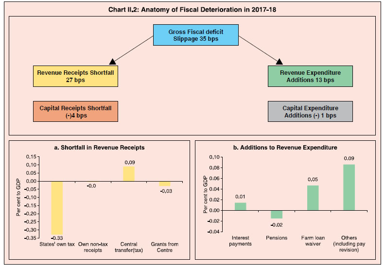 2.9 While 12 out of 29 states had budgeted fiscal deficits above the 3 per cent norm in 2017-18 (BE), the RE revealed that as many as 19 exceeded the norm. In fact the year 2017-18 saw a change from the previous few years with all deficit indicators worsening for SC states than that of NSC states and most SC states recording GFDs above the 3 per cent mark (Table II.5). | Table II.5: Deficit Indicators of State Governments: State-wise | | (Per cent) | | State | 2015-16 | 2016-17 | 2017-18 (RE) | 2018-19 (BE) | | RD/ GSDP | GFD/ GSDP | PD/ GSDP | RD/ GSDP | GFD/ GSDP | PD/ GSDP | RD/ GSDP | GFD/ GSDP | PD/ GSDP | RD/ GSDP | GFD/ GSDP | PD/ GSDP | | 1 | 2 | 3 | 4 | 5 | 6 | 7 | 8 | 9 | 10 | 11 | 12 | 13 | | I. Non-Special Category | 0.1 | 3.3 | 1.7 | 0.4 | 3.7 | 2.0 | 0.4 | 2.9 | 1.1 | 0.0 | 2.6 | 0.9 | | 1. Andhra Pradesh | 1.2 | 3.6 | 2.0 | 2.5 | 4.4 | 2.7 | 0.5 | 3.4 | 1.6 | -0.6 | 2.6 | 1.0 | | 2. Bihar | -3.3 | 3.2 | 1.3 | -2.5 | 3.8 | 1.9 | -0.3 | 7.2 | 5.2 | -3.9 | 2.0 | 0.1 | | 3. Chhattisgarh | -0.9 | 2.1 | 1.3 | -1.9 | 1.4 | 0.5 | -1.0 | 3.0 | 2.0 | -1.2 | 2.8 | 1.7 | | 4. Goa | -0.2 | 2.7 | 0.8 | -1.1 | 1.5 | -0.3 | -0.4 | 4.6 | 2.9 | -0.2 | 4.8 | 3.2 | | 5. Gujarat | -0.2 | 2.2 | 0.7 | -0.5 | 1.4 | -0.1 | -0.5 | 1.7 | 0.2 | -0.4 | 1.7 | 0.4 | | 6. Haryana | 2.4 | 6.5 | 4.8 | 2.9 | 4.8 | 2.9 | 1.4 | 2.8 | 0.9 | 1.2 | 2.9 | 0.8 | | 7. Jharkhand | -1.8 | 5.0 | 3.5 | -0.8 | 4.0 | 2.3 | -2.8 | 2.5 | 0.9 | -2.1 | 2.5 | 0.6 | | 8. Karnataka | -0.2 | 1.9 | 0.8 | -0.1 | 2.5 | 1.5 | 0.0 | 2.8 | 1.7 | 0.0 | 2.9 | 1.7 | | 9. Kerala | 1.7 | 3.2 | 1.2 | 2.5 | 4.3 | 2.3 | 1.9 | 3.4 | 1.4 | 1.7 | 3.2 | 1.2 | | 10. Madhya Pradesh | -1.1 | 2.7 | 1.1 | -0.6 | 4.3 | 2.9 | -0.1 | 3.4 | 1.7 | 0.0 | 3.3 | 1.7 | | 11. Maharashtra | 0.3 | 1.4 | 0.1 | 0.4 | 1.7 | 0.4 | 0.6 | 1.8 | 0.5 | 0.5 | 1.8 | 0.6 | | 12. Odisha | -3.1 | 2.1 | 1.1 | -2.5 | 2.5 | 1.4 | -2.1 | 3.5 | 2.3 | -2.2 | 3.4 | 2.2 | | 13. Punjab | 2.2 | 4.4 | 1.9 | 1.7 | 12.3 | 9.6 | 3.1 | 4.5 | 1.2 | 2.5 | 3.9 | 0.7 | | 14. Rajasthan | 0.9 | 9.2 | 7.5 | 2.4 | 6.1 | 3.8 | 2.4 | 3.5 | 1.1 | 1.9 | 3.0 | 0.7 | | 15. Tamil Nadu | 1.0 | 2.8 | 1.3 | 1.0 | 4.3 | 2.7 | 1.3 | 2.8 | 1.0 | 1.1 | 2.8 | 1.0 | | 16. Telangana | 0.0 | 3.3 | 1.9 | -0.2 | 5.5 | 4.1 | -0.2 | 3.2 | 1.7 | -0.7 | 3.5 | 2.1 | | 17. Uttar Pradesh | -1.3 | 5.2 | 3.3 | -1.6 | 4.5 | 2.4 | -1.4 | 3.1 | 0.8 | -1.8 | 3.0 | 0.8 | | 18. West Bengal | 1.0 | 2.3 | -0.2 | 1.5 | 2.4 | 0.0 | 0.9 | 2.4 | 0.2 | 0.0 | 1.7 | -0.2 | | II. Special Category | -1.4 | 2.1 | 0.1 | -1.2 | 3.0 | 0.9 | 0.6 | 6.6 | 4.5 | -2.4 | 3.4 | 1.3 | | 1. Arunachal Pradesh | -10.7 | -0.9 | -3.0 | -10.8 | -3.8 | -5.6 | -17.7 | 2.8 | 0.8 | -26.7 | 2.0 | -0.9 | | 2. Assam | -2.4 | -1.3 | -2.5 | 0.1 | 2.4 | 1.2 | 8.1 | 12.7 | 11.4 | -0.8 | 3.0 | 1.7 | | 3. Himachal Pradesh | -1.0 | 1.9 | -0.9 | -0.7 | 4.7 | 2.0 | 1.9 | 5.4 | 2.6 | 2.1 | 5.2 | 2.4 | | 4. Jammu and Kashmir | 0.5 | 6.8 | 3.6 | -1.6 | 4.7 | 1.2 | -8.1 | 3.9 | 0.8 | -8.1 | 4.5 | 1.8 | | 5. Manipur | -4.7 | 1.8 | -0.9 | -4.4 | 2.5 | 0.0 | -7.3 | 3.5 | 1.1 | -6.3 | 2.4 | 0.0 | | 6. Meghalaya | -2.7 | 2.1 | 0.3 | -2.1 | 2.5 | 0.6 | -2.0 | 3.8 | 1.8 | -1.5 | 3.4 | 1.5 | | 7. Mizoram | -7.2 | -2.7 | -5.1 | -6.2 | -1.3 | -3.2 | -5.9 | 3.2 | 1.5 | -6.3 | 1.0 | -0.5 | | 8. Nagaland | -2.3 | 3.0 | 0.1 | -3.5 | 1.3 | -1.5 | -0.1 | 6.6 | 3.6 | -1.8 | 3.2 | 0.1 | | 9. Sikkim | -0.8 | 3.1 | 1.5 | -4.4 | -0.5 | -2.2 | -5.9 | 3.5 | 1.8 | -2.7 | 3.0 | 1.0 | | 10. Tripura | -4.5 | 4.8 | 2.7 | -2.2 | 6.0 | 4.0 | 2.0 | 7.7 | 5.5 | -1.9 | 2.9 | 0.8 | | 11. Uttarakhand | 1.1 | 3.5 | 1.8 | 0.2 | 2.8 | 0.9 | 0.0 | 2.6 | 0.7 | 0.0 | 2.8 | 0.8 | | All States# | 0.0 | 3.1 | 1.5 | 0.3 | 3.5 | 1.9 | 0.4 | 3.1 | 1.3 | -0.2 | 2.6 | 0.9 | | Memo Item: | | 1. NCT Delhi | -1.6 | -0.2 | -0.8 | -0.8 | 0.2 | -0.3 | -0.6 | 0.3 | -0.2 | -0.6 | 0.4 | 0.0 | | 2. Puducherry | 0.8 | 2.5 | 0.3 | 0.3 | 1.9 | -0.2 | 0.1 | 1.9 | -0.3 | 0.0 | 1.3 | -0.8 | RE: Revised Estimates. BE: Budget Estimates. RD: Revenue Deficit. GFD : Gross Fiscal Deficit.
PD: Primary Deficit. GSDP: Gross State Domestic Product.
# As percentages to GDP
Note: Negative (-) sign in deficit indicators indicates surplus.
Source: Based on budget documents of state governments. | 2.10 Comparing the 2017-18 (RE) with 2016-17 (accounts), it is observed that while the consolidated states’ GFD at 3.1 per cent of GDP marks some consolidation over 3.5 per cent recorded in 2016-17, there was a deterioration in the revenue balance as revenue spending outpaced receipts and revenue deficit saw a more than 50 per cent growth (Table II.5 and II.6). | Table II.6: Variation in Major Items | | (₹ billion) | | Item | 2014-15 | 2015-16 | 2016-17 | 2017-18 (RE) | 2018-19 (BE) | Percent Variation | | 2017-18 RE over 2016-17 | 2018-19 BE over 2017-18 RE | | 1 | 2 | 3 | 4 | 5 | 6 | 7 | 8 | | I. Revenue Receipts (i+ii) | 15,915.8 | 18,328.8 | 20,464.0 | 24,577.2 | 28,129.9 | 20.1 | 14.5 | | (i) Tax Revenue (a+b) | 11,171.1 | 13,533.4 | 15,207.7 | 17,437.7 | 20,134.5 | 14.7 | 15.5 | | (a) Own Tax Revenue | 7,792.8 | 8,471.4 | 9,129.1 | 10,503.5 | 11,988.0 | 15.1 | 14.1 | | of which: Sales Tax | 4,942.7 | 5,282.4 | 5,874.5 | 4,309.7 | 3,085.6 | -26.6 | -28.4 | | (b) Share in Central Taxes | 3,378.4 | 5,061.9 | 6,078.6 | 6,934.2 | 8,146.6 | 14.1 | 17.5 | | (ii) Non-Tax Revenue | 4,744.7 | 4,795.5 | 5,256.3 | 7,139.5 | 7,995.4 | 35.8 | 12.0 | | (a) States' Own Non-Tax Revenue | 1,436.7 | 1,536.5 | 1,695.4 | 1,945.9 | 2,249.0 | 14.8 | 15.6 | | (b) Grants from Centre | 3,308.0 | 3,259.0 | 3,560.9 | 5,193.6 | 5,746.4 | 45.8 | 10.6 | | II. Revenue Expenditure | 16,372.9 | 18,382.7 | 20,868.9 | 25,188.0 | 27,837.8 | 20.7 | 10.5 | | of which: | | | | | | | | | (i) Development Expenditure | 10,403.9 | 11,811.4 | 13,404.6 | 16,122.9 | 17,508.1 | 20.3 | 8.6 | | of which: Education, Sports, Art and Culture | 3,154.3 | 3,494.9 | 3,869.3 | 4,312.5 | 4,979.2 | 11.5 | 15.5 | | Transport and Communication | 430.5 | 409.7 | 451.4 | 471.7 | 482.2 | 4.5 | 2.2 | | Power | 922.8 | 1,089.1 | 1,300.5 | 1,206.2 | 1,254.3 | -7.3 | 4.0 | | Relief on account of Natural Calamities | 180.6 | 327.4 | 280.0 | 299.3 | 210.5 | 6.9 | -29.7 | | Rural Development | 952.2 | 1,079.7 | 1,262.5 | 1,488.0 | 1,624.8 | 17.9 | 9.2 | | (ii) Non-Development Expenditure | 5,505.1 | 6,086.1 | 6,910.1 | 8,351.8 | 9,506.3 | 20.9 | 13.8 | | of which: Administrative Services | 1,199.5 | 1,302.1 | 1,455.8 | 1,765.1 | 2,075.4 | 21.2 | 17.6 | | Pension | 1,830.7 | 2,041.4 | 2,261.4 | 2,789.4 | 3,104.0 | 23.4 | 11.3 | | Interest Payments | 1,904.2 | 2,142.5 | 2,513.0 | 2,927.5 | 3,154.6 | 16.5 | 7.8 | | III. Net Capital Receipts # | 3,439.4 | 4,246.3 | 5,603.8 | 5,221.1 | 5,324.3 | -6.8 | 2.0 | | of which: Non-Debt Capital Receipts | 200.6 | 83.1 | 162.1 | 564.8 | 597.1 | 248.3 | 5.7 | | IV. Capital Expenditure $ | 3,015.5 | 4,236.0 | 5,100.5 | 5,097.1 | 5,754.4 | -0.1 | 12.9 | | of which: Capital Outlay | 2,719.1 | 3,333.8 | 3,921.9 | 4,707.1 | 5,377.9 | 20.0 | 14.3 | | of which: Capital Outlay on Irrigation and Flood Control | 555.8 | 685.2 | 832.6 | 945.8 | 1,118.2 | 13.6 | 18.2 | | Capital Outlay on Energy | 338.7 | 466.3 | 531.3 | 489.0 | 455.6 | -8.0 | -6.8 | | Capital Outlay on Transport | 663.1 | 788.5 | 948.0 | 1,079.9 | 1,111.1 | 13.9 | 2.9 | | Memo Item: | | | | | | | | | Revenue Deficit | 457.0 | 53.8 | 404.9 | 610.8 | -292.2 | 50.8 | -147.8 | | Gross Fiscal Deficit | 3,271.9 | 4,206.7 | 5,343.3 | 5,143.2 | 4,865.1 | -3.7 | -5.4 | | Primary Deficit | 1,367.8 | 2,064.2 | 2,830.3 | 2,215.7 | 1,710.6 | -21.7 | -22.8 | RE: Revised Estimates. BE: Budget Estimates.
# : It includes following items on net basis Internal Debt, Loans and Advances from the Centre, Inter-State Settlement, Contingency Fund, Small Savings, Provident Funds, Reserve Funds, Deposits and Advances, Suspense and Miscellaneous, Appropriation to Contingency Fund and Remittances.
$ : Capital Expenditure includes Capital Outlay and Loans and Advances by State Governments.
Note: 1. Negative (-) sign in deficit indicators indicates surplus.
2. Also see Notes to Appendices.
Source: Budget documents of state governments. | 2.11 Expenditure on the revenue account surged in 2017-18, on both development and non-development heads. Higher spending on sectors such as housing, medical and public health and crop husbandry were the major propellers of development expenditure. Non-development expenditure was pushed up by committed expenditures – pension payments; spending on administrative services, essentially led by pay commission recommendations; and interest payments driven up by rising market borrowings as well as yields (Chart II.3). 2.12 While capital expenditure stagnated in 2017-18 (RE), capital outlay showed an impressive growth of 20 per cent over 2016-17 in respect of irrigation, flood control and transport, but declined for energy sub-sectors. The decline in overall capex reflects the termination of UDAY scheme. Capital receipts also declined due to repayment of loans and advances (Table II.6). 4. Budget Estimates: 2018-19 2.13 For 2018-19, states have budgeted for a consolidated GFD of 2.6 per cent of GDP, with 11 states planning to remain above the 3 per cent threshold (Chart II.4). Consolidation is mainly expected to accrue from the revenue balance, which is expected to post a surplus of 0.2 per cent of GDP in 2018-19 (BE) as against a deficit of 0.4 per cent in 2017-18 (RE) (Chart II.1). Capital outlay is envisaged to account for more than 100 per cent of the fiscal deficit, indicative of the inclination to bring about improvement in the quality of the deficit (Table II.7). States have also projected an increase in their reliance on market borrowings to about 91 per cent of GFD, in line with the recommendation of the fourteenth Finance Commission (FC-XIV). 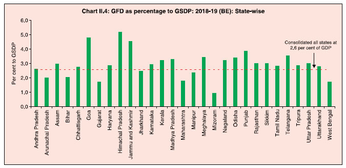
| Table II.7: Decomposition and Financing Pattern of Gross Fiscal Deficit | | (Per cent to GFD) | | Item | 2014-15 | 2015-16 | 2016-17 | 2017-18 (RE) | 2018-19 (BE) | | 1 | 2 | 3 | 4 | 5 | 6 | | Decomposition (1+2+3-4) | 100.0 | 100.0 | 100.0 | 100.0 | 100.0 | | 1. Revenue Deficit | 14.0 | 1.3 | 7.6 | 11.9 | -6.0 | | 2. Capital Outlay | 83.1 | 79.3 | 73.4 | 91.5 | 110.5 | | 3. Net Lending | 3.3 | 19.7 | 19.1 | -3.3 | -4.3 | | 4. Non-debt Capital Receipts | 0.4 | 0.3 | 0.1 | 0.1 | 0.2 | | Financing (1 to 8) | 100.0 | 100.0 | 100.0 | 100.0 | 100.0 | | 1. Market Borrowings | 63.1 | 61.4 | 65.8 | 74.9 | 90.6 | | 2. Loans from Centre | 0.3 | 0.2 | 1.0 | 2.3 | 2.9 | | 3. Special Securities issued to NSSF/Small Savings | 7.3 | 6.4 | -6.0 | -6.1 | -6.8 | | 4. Loans from LIC, NABARD, NCDC, SBI and Other Banks | 1.2 | 3.9 | 8.2 | 4.0 | 4.8 | | 5. Provident Fund | 8.3 | 7.9 | 7.4 | 5.5 | 6.8 | | 6. Reserve Funds | 0.2 | 0.1 | 3.9 | 2.1 | 3.5 | | 7. Deposits and Advances | 9.0 | 5.5 | 8.0 | 2.1 | 4.3 | | 8. Others | 10.6 | 14.5 | 11.8 | 15.3 | -6.2 | RE : Revised Estimates. BE : Budget Estimates.
Note : 1. See Notes to Appendix Table 9.
2. ‘Others’ include Compensation and Other Bonds, Loans from Other Institutions, Appropriation to Contingency Fund, Inter-State Settlement and Contingency Fund.
Source : Budget documents of state governments. | Revenue Receipts 2.14 Revenue receipts are expected to go up on account of central transfers and states’ own taxes comprising states’ GST and other commodity taxes (Table II.3 and Chart II.5). 2.15 Notwithstanding some uncertainty in revenues in 2017-18 associated with the GST implementation, state-wise analysis suggests better prospects going forward (Box II.1). Box II.1:
Goods and Services Tax (GST) – A State Level Analysis Twelve years after the implementation of value added tax (VAT) in 2005, India rolled out the goods and services tax (GST) on July 1, 2017. The GST is a destination-based single tax on the supply of goods and services by manufacturers to the consumer. The GST is by far the largest tax reform in India paving the way for a single national market. It is expected to raise international competitiveness and attract stable foreign investment. GST is also likely to have a salubrious impact on state finances in the medium run as it would prevent leakages and broaden the indirect tax base. The various institutional reforms accompanying the new regime, viz., greater cooperation between centre and states on tax policy and exemptions as well as larger shareable pool of taxes is expected to infuse new life into cooperative federalism. Looking at the states’ budget data, since only few states had budgeted for GST in 2017-18 BE, GST revenues have gone up in the revised estimates (RE). However, this increase could not compensate for the decline in sales tax revenues in 2017-18 RE vis-à-vis BE resulting in a net slippage of about 0.4 per cent of GDP in tax revenues (Table 1). For 2018-19 BE, states as expected have budgeted higher state GST (SGST) and lower sales tax. It may be noted that the GST revenues as reported in RE of state budgets is on the lower side as not all have reported the components of GST uniformly across states. For instance, only 21 states have reported revenue from central GST (CGST) in 2017-18 while only 2 have reported compensation cess (Table 2). Even for 2018-19, some states have not budgeted for some of these components. The quarterly data on tax revenues for select six states (with comparable monthly data available in CAG) indicate that while tax revenues for some of these states moderated during the second and third quarter of 2017-18, it has picked up significantly in the Q4 2017-18. The pick-up is significant even after accounting for the usual seasonal uptick in Q4 of each year (Table 3). This observed buoyancy in tax revenues augurs well for the states in getting back to the path of fiscal consolidation over the medium term. | Table 1: Disaggregated States' Own Tax Revenue | | (Per cent to GDP) | | Item | 2014-15 | 2015-16 | 2016-17 | 2017-18 (BE) | 2017-18 (RE) | 2018-19 (BE) | | 1 | 2 | 3 | 4 | 5 | 6 | 7 | | TOTAL REVENUE | 12.8 | 13.3 | 13.4 | 14.9 | 14.7 | 15.0 | | TAX REVENUE | 9.0 | 9.8 | 10.0 | 10.6 | 10.4 | 10.8 | | State's Own Tax Revenue | 6.3 | 6.2 | 6.0 | 6.6 | 6.3 | 6.4 | | Of which: | | | | | | | | a. Taxes on Property and CapitalTransactions | 0.8 | 0.8 | 0.7 | 0.7 | 0.7 | 0.7 | | b. Taxes on Commodities and Services | 5.4 | 5.4 | 5.3 | 5.8 | 5.5 | 5.7 | | Of which Sales Tax | 4.0 | 3.8 | 3.9 | 4.1 | 2.6 | 1.6 | | State Excise | 0.7 | 0.7 | 0.7 | 0.8 | 0.7 | 0.8 | | Taxes on Vehicles | 0.3 | 0.3 | 0.3 | 0.4 | 0.4 | 0.4 | | SGST | 0.0 | 0.0 | 0.0 | 0.3 | 1.5 | 2.6 | | Source: Budget documents of state governments |
| Table 2: GST Collection: Stylised Facts | | | 2017-18 (RE) (₹ Billion) | Number of States Reported | 2018-19 BE (₹ Billion) | Number of States Reported | | 1 | 2 | 3 | 4 | 5 | | SGST | 2,559.3 | 26 | 4,845.8 | 28 | | CGST | 523.7 | 21 | 2,036.7 | 23 | | IGST | 642.0 | 24 | 675.9 | 25 | | Compensation Cess | 22.0 | 4 | 36.1 | 4 | Note: The GST cess (Compensation to State) Act, 2017, is a compensation cess that is levied on specific items and services for compensation to the States for the loss of revenue on account of implementation of the GST in pursuance of the provisions of the Constitution Act, 2016. Thus, States remain protected on that account for first 5 years of GST implementation.
Source: Budget documents of state governments. |
To sum up, states’ own tax revenue during 2017-18 (RE) suffered a marginal dip over the BE levels. Going forward, the new tax regime will likely exploit the higher tax revenue elasticities and improve the fiscal situation of states through enhanced tax base and efficiency. | Table 3: Tax Revenue in Six Selected States | | (Per cent to GDP) | | | West Bengal | Punjab | Odisha | MP | HP | Gujarat | | 1 | 2 | 3 | 4 | 5 | 6 | 7 | | 2015-16:Q1 | 0.41 | 0.27 | 0.31 | 0.55 | 0.06 | 0.60 | | 2015-16:Q2 | 0.53 | 0.24 | 0.31 | 0.51 | 0.08 | 0.57 | | 2015-16:Q3 | 0.53 | 0.25 | 0.30 | 0.52 | 0.07 | 0.52 | | 2015-16:Q4 | 0.82 | 0.24 | 0.37 | 0.68 | 0.08 | 0.59 | | 2016-17:Q1 | 0.41 | 0.23 | 0.29 | 0.52 | 0.07 | 0.51 | | 2016-17:Q2 | 0.45 | 0.23 | 0.30 | 0.50 | 0.07 | 0.55 | | 2016-17:Q3 | 0.69 | 0.24 | 0.30 | 0.55 | 0.08 | 0.51 | | 2016-17:Q4 | 0.78 | 0.27 | 0.44 | 0.78 | 0.08 | 0.62 | | 2017-18:Q1 | 0.30 | 0.26 | 0.31 | 0.56 | 0.08 | 0.61 | | 2017-18:Q2 | 0.63 | 0.21 | 0.38 | 0.52 | 0.06 | 0.51 | | 2017-18:Q3 | 0.47 | 0.26 | 0.29 | 0.47 | 0.07 | 0.49 | | 2017-18:Q4 | 0.99 | 0.28 | 0.57 | 0.66 | 0.08 | 0.67 | | Source: Comptroller and Auditor General of India (CAG). | |
Expenditure Pattern 2.16 Surplus in the revenue account is budgeted to accrue on account of a lower increase in revenue expenditure in 2018-19 vis-a-vis 2017-18 (RE) with regard to farm loan waivers (Chart II.5). Non-development expenditure is estimated to rise in 2018-19, backed by committed expenditure on administrative services. Development expenditure, however, has been projected to moderate/decline in some sectors - rural development and relief on account of natural calamities - while higher allocations have been made for education, sports, art and culture (Table II.6). 2.17 Capital outlay is expected to grow slower at about 14 per cent in 2018-19 as against the growth of 20 per cent a year ago. Spending on energy sub-sector has been programmed to decline, while higher allocations have been made for the ‘medium and major irrigation and flood control’ subsectors. 2.18 Social sector expenditure (SSE)5 has a strong link with overall economic development, particularly in the medium to long term. SSE is budgeted to increase in 2018-19 as a proportion to aggregate expenditure over 2017-18 (RE) (Chart II.6). As a proportion to states’ respective GSDP, twelve states have budgeted to increase SSE (Statement 35 for 2018-19). 2.19 The composition of expenditure on social services points toward a shift in expenditure from education and health to other types of expenditure such as water supply and sanitation, housing and urban development, though the former accounts for around 55 per cent of total social service spending (Table II.8). Recent initiatives such as the Swachh Bharat Mission, affordable housing schemes and the smart cities mission appear to be the major drivers of this shift. | Table II.8: Composition of Expenditure on Social Services (Revenue and Capital Accounts) | | (Per cent to expenditure on social services) | | Item | 2014-15 | 2015-16 | 2016-17 | 2017-18 (RE) | 2018-19 (BE) | | 1 | 2 | 3 | 4 | 5 | 6 | | Expenditure on Social Services (a to l) | 100.0 | 100.0 | 100.0 | 100.0 | 100.0 | | (a) Education, Sports, Art and Culture | 46.2 | 44.0 | 42.9 | 39.7 | 41.0 | | (b) Medical and Public Health | 11.6 | 11.4 | 11.5 | 11.5 | 11.5 | | (c) Family Welfare | 2.2 | 2.0 | 2.0 | 2.0 | 2.0 | | (d) Water Supply and Sanitation | 5.6 | 5.6 | 6.2 | 6.5 | 6.2 | | (e) Housing | 3.1 | 3.1 | 3.5 | 4.7 | 4.6 | | (f) Urban Development | 5.9 | 6.4 | 7.9 | 8.8 | 8.8 | | (g) Welfare of SCs, ST and OBCs | 6.8 | 7.1 | 7.0 | 7.9 | 8.2 | | (h) Labour and Labour Welfare | 1.1 | 0.9 | 0.8 | 1.0 | 1.0 | | (i) Social Security and Welfare | 10.6 | 11.4 | 10.9 | 10.8 | 10.6 | | (j) Nutrition | 2.9 | 2.6 | 2.5 | 2.5 | 2.5 | | (k) Expenditure on Natural Calamities | 2.6 | 4.0 | 3.0 | 2.6 | 1.7 | | (l) Others | 1.4 | 1.4 | 1.8 | 2.0 | 1.9 | RE: Revised Estimates. BE: Budget Estimates.
Source : Budget documents of the state governments. | 5. Outstanding Liabilities of State Governments 2.20 Outstanding liabilities of states have been growing at double digits, barring in 2014-15 (Table II.9). The issuance of UDAY bonds in 2015-16 and 2016-17, farm loan waivers and the implementation of pay commission awards led to higher debt- GDP ratio at 24.0 per cent in 2017-18 (RE) which is expected to rise to 24.3 per cent in 2018-19 (BE). State-wise data reveal that the debt-GSDP ratio increased in 2018-19 for 16 states (Statement 20). | Table II.9: Outstanding Liabilities of State Governments | | Year (end-March) | Amount (₹ billion) | Annual Growth | Debt /GDP | | (Percent) | | 1 | 2 | 3 | 4 | | 2012 | 19,939.2 | 9.0 | 22.8 | | 2013 | 22,102.5 | 10.8 | 22.2 | | 2014 | 24,712.6 | 11.8 | 22.0 | | 2015 | 27,037.6 | 9.4 | 21.7 | | 2016 | 32,181.3 | 19.0 | 23.4 | | 2017 | 36,293.1 | 12.8 | 23.8 | | 2018 (RE) | 40,220.8 | 10.8 | 24.0 | | 2019 (BE) | 45,408.5 | 12.9 | 24.3 | RE: Revised Estimates. BE: Budget Estimates.
Source : 1. Budget documents of state governments.
2. Combined Finance and Revenue Accounts of the Union and the State Governments in India, Comptroller and Auditor General of India.
3. Ministry of Finance, Government of India.
4. Reserve Bank records.
5. Controller General of Accounts (CGA). | 2.21 Despite the rising path of states’ indebtedness, their interest payment to revenue receipts (IP-RR) ratio has remained unchanged on account of revenue receipts compensating for the increase in interest payments (Chart II.7). Composition of Debt6 2.22 Of this outstanding debt, market borrowings constituted 76.2 per cent at end- March 2018 and is projected to increase to 77.0 per cent at end-March 2019 (Table II.10). Within this rising debt profile, loans from banks and financial institutions stagnated at around 4 per cent and the share of the National Small Savings Fund (NSSF) continued to decline. Similarly, loans from the centre and public accounts items are also declining gradually and getting replaced by market loans. | Table II.10: Composition of Outstanding Liabilities of State Governments (As at end-March) | | (Per cent) | | Item | 2014 | 2015 | 2016 | 2017 | 2018 RE | 2019 BE | | 1 | 2 | 3 | 4 | 5 | 6 | 7 | | Total Liabilities (1 to 4) | 100.0 | 100.0 | 100.0 | 100.0 | 100.0 | 100.0 | | 1. Internal Debt | 66.2 | 69.7 | 72.0 | 75.3 | 76.2 | 77.0 | | of which: (i) Market Loans | 42.5 | 46.9 | 47.1 | 51.2 | 54.7 | 58.2 | | (ii) Special Securities Issued to NSSF | 19.8 | 19.0 | 16.8 | 14.0 | 11.8 | 9.8 | | (iii) Loans from Banks and Financial Institutions | 3.6 | 3.5 | 4.4 | 3.9 | 4.0 | 4.1 | | 2. Loans and Advances from the Centre | 5.9 | 5.4 | 4.6 | 4.2 | 4.1 | 4.0 | | 3. Public Account (i to iii) | 27.7 | 24.6 | 23.3 | 20.3 | 19.6 | 18.9 | | (i) State Provident Funds, etc. | 12.4 | 11.8 | 10.9 | 9.9 | 9.6 | 9.2 | | (ii) Reserve Funds | 6.0 | 3.7 | 4.3 | 2.0 | 2.0 | 2.2 | | (iii) Deposits & Advances | 9.3 | 9.1 | 8.1 | 8.5 | 7.9 | 7.5 | | 4. Contingency Fund | 0.1 | 0.2 | 0.1 | 0.1 | 0.1 | 0.1 | RE: Revised Estimate. BE: Budget Estimate.
Source: Same as that for Table II.9. | 2.23 During 2017-18, upside risks to inflation, fiscal slippages, farm loan waivers and global factors such as increasing crude oil prices and monetary policy normalisation by the US were the major factors impacting the yields on state development loans (SDLs)7. 2.24 Pursuant to the recommendation of the FC-XIV, states (barring Delhi, Madhya Pradesh, Kerala and Arunachal Pradesh) have been excluded from the National Small Savings Fund (NSSF) financing facility from 2016-17. The consequent increase in their market borrowings has imposed large redemption pressures, exacerbating the debt management burden. The share of market borrowings in financing GFD has increased from 61.4 per cent in 2015-16 to 74.9 per cent in 2017-18 (RE) and is projected to rise further to 90.6 per cent in 2018-19 (BE) (Table II.7) mainly due to the termination of the NSSF financing facility. 2.25 The number of issuances of state development loans (SDL) has almost doubled between 2012-13 and 2017-18 even as average issue size has gone up (Table II.11). | Table II.11: Gross and Net Market Borrowing of State Government | | | Gross Market Borrowings (₹ Billion) | Net Market Borrowings (₹ Billion) | Number of Issuances | Average Size (₹ Billion) | Weighted Average Yield (in per cent) | | 1 | 2 | 3 | 4 | 5 | 6 | | 2012-13 | 1,772.8 | 1,466.5 | 222 | 8.0 | 8.84 | | 2013-14 | 1,966.6 | 1,645.9 | 253 | 7.8 | 9.18 | | 2014-15 | 2,408.4 | 2,074.6 | 283 | 8.5 | 8.58 | | 2015-16 | 2,945.6 | 2,593.7 | 298 | 9.9 | 8.28 | | 2016-17 | 3,819.8 | 3,426.5 | 337 | 11.3 | 7.48 | | 2017-18 | 4,191.0 | 3,402.8 | 411 | 10.2 | 7.60 | 2.26 The wedge in the net and gross market borrowings indicates the increasing redemption pressure, which is likely to persist (Chart II.8). Post global financial crisis (GFC), the market borrowing of states increased mainly due to the additional fiscal space given to states as part of stimulus measures. Since states normally issue plain vanilla bonds with the maturity of 10 years, the redemption pressures increased from 2017-18, implying that the borrowings of states are expected to soar. There was no UDAY issuance during the year 2017-18. 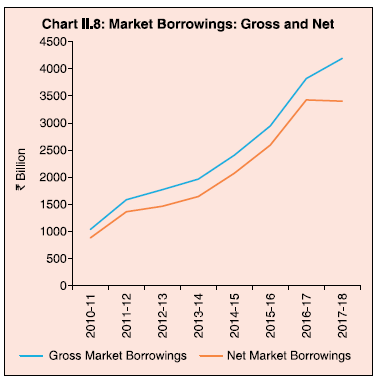 2.27 Among the NSC states, Maharashtra (10.7 per cent), Uttar Pradesh (9.9 per cent), Tamil Nadu (9.7 per cent) and West Bengal (8.8 per cent) had the largest shares in market borrowings during 2017-18. Among the SC states, Assam (1.9 per cent), Himachal Pradesh (1.1 per cent), Jammu and Kashmir (1.5 per cent) and Uttarakhand (1.6 per cent) were the major borrowers (Chart II.9). The growth of gross market borrowing of SC states at 58.9 per cent during 2017-18 outstripped that of NSC states by a wide margin (7.0 per cent). Maturity Profile of State Government Securities 2.28 The maturity profile of states’ debt indicates near to medium-term redemption pressures, which is likely to rise continuing from current year and reach a peak in 2026-27 (Chart II.10). 2.29 At end March 2018, 67.2 per cent of the outstanding SDLs were in the residual maturity bucket of five years and above (Table II.12). About 16.7 per cent of outstanding SDLs will mature in the next three years, keeping redemption pressure high in the near future. | Table II.12: Maturity Profile of Outstanding State Government Securities (As at end-March 2018) | | State | Per cent of Total Amount Outstanding | | 0-1 years | 1-3 years | 3-5 years | 5-7 years | Above 7 years | | 1 | 2 | 3 | 4 | 5 | 6 | | I. Non-Special Category | | | | | | | 1. Andhra Pradesh | 4.4 | 13.4 | 15.3 | 21.5 | 45.3 | | 2. Bihar | 4.5 | 7.3 | 15.1 | 19.8 | 53.4 | | 3. Chhattisgarh | 0.0 | 2.6 | 6.1 | 26.9 | 64.4 | | 4. Goa | 5.5 | 9.8 | 15.3 | 19.5 | 49.9 | | 5. Gujarat | 6.3 | 14.4 | 21.2 | 19.1 | 39.1 | | 6. Haryana | 2.7 | 6.9 | 19.8 | 27.2 | 43.5 | | 7. Jharkhand | 3.8 | 6.1 | 15.4 | 23.3 | 51.3 | | 8. Karnataka | 5.9 | 6.4 | 8.4 | 26.6 | 52.7 | | 9. Kerala | 4.8 | 9.5 | 17.7 | 22.5 | 45.6 | | 10. Madhya Pradesh | 4.9 | 10.7 | 10.1 | 18.4 | 55.9 | | 11. Maharashtra | 7.0 | 11.8 | 19.8 | 19.3 | 42.1 | | 12. Odisha | 4.2 | 14.9 | 21.1 | 13.4 | 46.3 | | 13. Punjab | 4.7 | 17.0 | 23.3 | 16.9 | 38.1 | | 14. Rajasthan | 7.5 | 15.8 | 15.2 | 20.1 | 41.5 | | 15. Tamil Nadu | 4.5 | 9.8 | 14.4 | 20.0 | 51.3 | | 16. Telangana | 3.9 | 9.7 | 13.3 | 16.4 | 56.6 | | 17. Uttar Pradesh | 5.0 | 13.2 | 13.5 | 13.6 | 54.7 | | 18. West Bengal | 5.7 | 11.7 | 19.5 | 19.6 | 43.5 | | II. Special Category | | | | | | | 1. Arunachal Pradesh | 1.1 | 3.4 | 8.8 | 23.2 | 63.5 | | 2. Assam | 11.2 | 12.1 | 1.3 | 13.1 | 62.3 | | 3. Himachal Pradesh | 8.6 | 11.7 | 13.4 | 19.8 | 46.5 | | 4. Jammu and Kashmir | 5.9 | 14.9 | 19.3 | 14.2 | 45.7 | | 5. Manipur | 7.5 | 18.8 | 10.5 | 20.0 | 43.3 | | 6. Meghalaya | 5.0 | 8.9 | 13.5 | 17.4 | 55.2 | | 7. Mizoram | 5.3 | 18.2 | 21.0 | 21.2 | 34.3 | | 8. Nagaland | 6.8 | 13.6 | 16.9 | 16.6 | 46.1 | | 9. Sikkim | 8.1 | 9.1 | 3.7 | 15.1 | 64.1 | | 10. Tripura | 3.0 | 12.4 | 18.4 | 13.6 | 52.6 | | 11. Uttarakhand | 3.8 | 6.0 | 11.8 | 18.4 | 60.0 | | All States | 5.3 | 11.4 | 16.1 | 19.6 | 47.6 | | Source: Reserve Bank records. | 2.30 During 2017-18, 9 states and the Union Territory of Puducherry issued non-standard securities with a maximum maturity of 25 years. Pursuing the strategy of passive consolidation, states like Maharashtra, Tamil Nadu and Odisha undertook reissuances during 2017-18, thereby creating critical mass to enable trading of securities in the secondary market. Liquidity Position and Cash Management 2.31 Several states have been accumulating sizeable cash surpluses in recent years, involving a negative carry8 on interest rates. As on March 31, 2018 states’ outstanding intermediate treasury bills (ITBs)9 stood at ₹1,508.7 billion and the stock of auction treasury bills (ATBs)10 was placed at ₹621 billion. States’ availment of ways and means advances (WMA) and overdrafts (ODs) rose in 2017-18 in comparison to the preceding year (Chart II.11). This increase was mainly due to heavy dependence on this facility by certain states due to state specific reasons. 6. Concluding Observations 2.32 To sum up, states’ fiscal position deteriorated during 2015-16 and 2016-17 due to the states taking over of Discom debt under UDAY schemes. Consequently, their consolidated fiscal deficit rose above the FRBM threshold level. As per the revised estimates, GFD-GDP ratio continued to remain above the FRBM threshold during 2017-18 due to shortfall in revenue receipts and higher revenue expenditure from implementation of farm loan waivers and the pay commission recommendations on salaries and pensions. 2.33 States have budgeted for a revenue surplus in 2018-19 and a lower fiscal deficit. Going forward, fiscal risk may emanate for many states going for election during the year, continuing announcements and rollouts of farm loan waivers as well as the implementation of the pay commission awards by some states. If the likely slippage is reflected in higher borrowing requirements for 2018-19, there could be a concomitant impact on borrowing costs. Revenue mobilisation remains the key towards attaining the budgeted targets. As the GST stabilises, it should boost states’ revenue capacity and support the resumption of fiscal consolidation. The cushion provided by compensation cess by the Centre for any interim shortfall may help smooth state finances from the revenue front. Nevertheless, better fiscal marksmanship and efficiency of expenditures appear essential to providing robustness to state finances if revenue receipts end up again in shortfall relative to budgeted levels.
|