Press Release RBI Working Paper Series No. 02
Non-Linear, Asymmetric and Time-Varying Exchange Rate Pass-Through:
Recent Evidence from India @Michael Debabrata Patra
Jeevan Kumar Khundrakpam
and
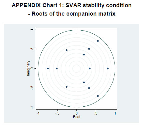
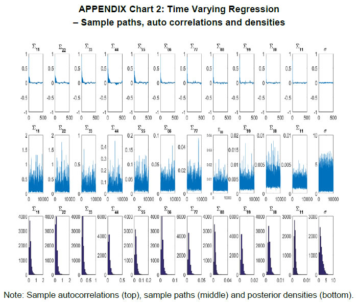
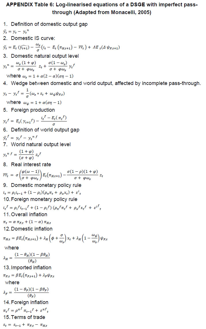
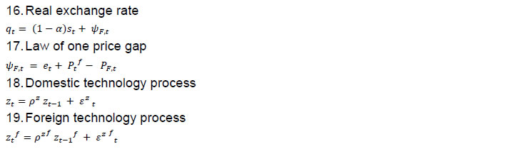
Joice John Abstract Exploring nonlinearities and time variations in exchange rate pass-through (ERPT) to consumer prices in India for the period from April 2005 to March 2016, this paper finds ERPT is asymmetric with pass-through from small depreciations being the strongest. ERPT to consumer inflation has declined in recent years in an environment of low inflation and declining trade openness. A DSGE model calibrated for the Indian economy with open economy features suggests that non-linear and time-varying ERPT poses challenges for monetary policy in terms of imported inflation and policy transmission. Key words: Exchange rate pass-through, Time-varying parameter regression. JEL classification: C32, E42, F31, F33. For an open2, inflation targeting, emerging market economy (EME) like India, exchange rate pass through (ERPT) to domestic prices is a key policy parameter for at least two important reasons. First, it has implications for the central bank's goal variable - inflation formation. Also, welfare effects working through consumers' disposable incomes and corporations' input costs/profit margins feed back into informing the setting of optimal monetary policy. Secondly, it influences the degrees of freedom available for conducting monetary policy in pursuit of domestic objectives - should the central bank sacrifice independence and respond to an exchange rate change even though it is not targeting the exchange rate? Yet, the inflation target itself could be threatened by the exchange rate change! Instantly, the trilemma comes alive. Quite naturally, the role of ERPT in the conduct of monetary policy has attracted prolific research attention; we have been chasing this mirage for over a decade (Khundrakpam, 2007; Patra and Kapur, 2012; Patra et al., 2014; John, 2015). The impetus for this surge of interest developed as this literature slipped its microeconomic moorings in industrial organisation in the late 1990s, led by an influential view that ERPT is endogenous to the monetary policy regime (Taylor, 2000). Since then too, the literature has shed its predominantly advanced economy focus and has acquired an abiding interest in ERPT in emerging economies. Repetitive visitations of generations of currency crises since the 1990s have not deterred EMEs from adopting floating exchange rate regimes and 'managing' them in preference to 'fixing', dispelling influential scepticism embodied in the fear of floating (Calvo and Reinhart, 2000; 2002) and the loss of monetary policy independence. It turned out that they had found the circuit-breaker - inflation targeting! The commitment to a numerical inflation target, and the collateral credibility it brought, anchored expectations and kept inflation variance subdued. Consequently, ERPT itself moderated for EMEs, suggesting reverse causality – from the monetary policy regime to ERPT, a la Taylor! In the ultimate analysis, ERPT is an empirical issue. The eclectic policy maker having to deal with it on operational terms is naturally wary about choice of methodology, controls, restrictions, time frame and stability of the estimates over space and time. Just as the empirical literature was coalescing around a settled position - that ERPT is delayed and incomplete; that it is low and stable in advanced economies (AEs), higher but declining in EMEs (Devereux and Yetman, 2008; Mihaljek and Klau, 2008; Lopez-Villavicencio and Mignon, 2016) – one strand has put a finger to the wound. Since the taper tantrum of the summer of 2013, global spillovers from ultra-accommodative monetary policies of systemic central banks have triggered large and sudden risk-on-risk-off swings in investor sentiment and asset prices, especially exchange rates. In this setting, evidence has been turned in on higher exchange rate volatility being associated with higher ERPT and axiomatically, with higher inflation variability (Campa and Goldberg, 2005; Bussiere, 2013; Cheikh and Rault, 2015; Jasova et al., 2016). Consequently, the standard approach of estimating ERPT as linear and symmetric could be biased towards overestimation as it would also pick up changes in exchange rate volatility. In contrast to the relative neglect in the standard literature, recent studies are putting out persuasive evidence that non-linearities cannot be neglected. Price rigidities and pricing to market strategies are found to impart convexity to ERPT, while switching costs - low elasticity of substitution between domestic and foreign goods - could give it concavity (Bussiere, 2013). One variant of non-linearity takes the form of asymmetries in ERPT. Asymmetric effects can be directional - the proportionate pass through of depreciations to inflation is different from that of appreciations (Khundrakpam, 2007). Also, there is compelling evidence that while the direction of asymmetry may vary at the firm level, size does matter - inflation may respond to large exchange rate changes differently than to small changes (Pollard and Coughlin, 2004). It has also been argued that the mainstream empirical literature captures only time-invariant factors - such as firms' pricing power - through fixed effects (Cheikh and Rault, 2015; Jasova et al., 2016). In reality, ERPT is determined by factors such as the stage of the economic cycle; monetary policy regime shifts; the market structure; and the composition of imports; all of which produce secular movements. Consequently, it becomes important to assess the stability of ERPT estimates over time. By abstracting the possibility of temporal shifts in the relationship between the exchange rate and macro variables, the mainstream literature embeds bias (Mumtaz and Sunder-Plassman, 2013). This is of particular relevance in periods characterised by large shocks, changes in transmission channels and regime shifts which are unlikely to be accounted for by a fixed-coefficient model. Against this backdrop, let’s cut to the chase and set out this paper’s motivation. As explained in the foregoing, topical interest has been revived by empirical evidence of changes in ERPT in the period following the global financial crisis (GFC). Drawing from these findings, exploring non-linear, asymmetric and time-varying properties of ERPT is the main driving force of this paper. The basic premise is that if these aspects are statistically significant, ignoring them will produce estimates of ERPT which reflect averages of the past and are, therefore, biased. The reference point for this effort is Khundrakpam (2007), which undertook a systematic examination of the behaviour of ERPT in India during 1991-2005. Investigating non-linearities in a framework encapsulating firms’ profit-maximising price-setting behaviour, it offered robust empirical evidence of higher ERPT for appreciations than for depreciations, and for small changes in the exchange rate over larger ones. Updating Khundrakpam (2007) and extending it to revisit non-linearities in ERPT in the post-global financial crisis period is empirically interesting because of the changing inflation dynamics in India in recent years, characterised by high volatility in food prices and exchange rates triggered by the incidence of supply shocks and financial market turbulence, respectively. Another motivation of the paper is to contribute country-specific evidence. India provides near-laboratory conditions, with stylised evidence suggesting a close interaction between exchange rate volatility and macroeconomic fundamentals - India has transitioned from the so-called 'fragile five' of 2013 to becoming a preferred habitat for capital flows to EMEs. Furthermore, the monetary policy framework in India went through a regime shift with the de facto adoption of flexible inflation targeting (FIT) from 2014 [de jure FIT was instituted in mid-2016, but in the years leading up to it, the Reserve Bank of India (RBI) set about preparing the ground and entrenching the pre-conditions for the new framework, including by developing the intellectual edifice (RBI, 2014) and by setting up informal numerical inflation targets in order to ensure a glide path into the formal regime]. Arguably, this experience has a generalised flavour that adds variety to the burgeoning literature on ERPT in EMEs. In this context, the objective of gleaning implementable policy advice assumes importance from our point of view. Non-linearities in ERPT have typically been examined for panels/groups of countries, the exceptions being time-varying parameter estimates for South Africa (Jooste and Jhaveri, 2013) and for Jamaica, Trinidad and Tobago, Mexico and Brazil (McFarlane, 2009). As pointed out in recent contributions, these panels do not offer any direct policy implications for individual countries (Jasova et al., 2017). Moreover, country experiences could question the conventional wisdom – in the case of Japan, there is recent empirical evidence of a resurgence in ERPT attributable to changes in production structure, the rising share of intermediate goods in production and consequent changes in price-setting behaviour (Shioji, 2014; 2015; Hara et al., 2015). A contribution in this paper is the estimation of ERPT for India on the basis of the first national consumer price index (CPI), instead of the wholesale price index/sectoral CPIs used in earlier work. To the best of our knowledge, this is the first attempt to study ERPT in India using the newly compiled CPI. In doing so, we also aim to tease out implications that can enliven the ongoing discussion on India’s new monetary policy framework, which has adopted headline CPI inflation as the numeraire to define its nominal anchor. We also address methodological questions thrown up in the literature such as the misspecification problem associated with estimations based on first differences, the identification of thresholds for exchange rate changes in the context of asymmetries and the dynamic adjustment of prices that tend to get ignored by assuming exogeneity of the exchange rate. We also validate the results for robustness in a structural vector auto regression (SVAR) framework. We estimate a non-linear functional form to identify threshold levels of exchange rate changes that impact ERPT and employ a time-varying parameter (TVP) model to allow parametric changes over time. The main findings of the paper can be summarised as follows: ERPT turns out to be lower in the post-2014 period than in the years prior to it. Declining levels of inflation and inflation variability, relatively subdued exchange rate volatility and a fall in the degree of openness embodied in the ratio of trade to GDP in this period contribute to lower ERPT. There are non-linearities in ERPT, which have implications for the conduct of monetary policy as they influence the responsiveness of inflation and output gaps to policy impulses. Illustratively, small depreciations produce relatively high ERPT and stronger monetary transmission, although global shocks could overwhelm steady state effects. These policy implications are examined by calibrating an open economy dynamic stochastic general equilibrium (DSGE) model of the Indian economy. The rest of the paper is organised into five sections. Section II presents the empirical framework and methodology. Section III parses the empirical results and drills into aspects of robustness of estimation. Section IV employs a small DSGE model to extract policy inferences that are of significance for India and can be broad-based to fit the EME experience of recent times. Section V concludes. II. Empirical Framework and Methodology ERPT to domestic inflation can be conceptualised as a two-stage process – (i) the change in import prices due to a unit change in the exchange rate, followed by (ii) the change in consumer prices via producer prices due to a unit change in import prices. In the literature, a partial equilibrium micro-founded mark-up equation (a la Campa and Goldberg, 2005) has emerged as the standard empirical specification for estimating first-stage ERPT. More recent efforts have sought to generalise and extend the standard model (Aron et al., 2014). Drawing on the latter, the reduced form of the set of equations that determine first-stage ERPT can be written as:  Variations in mupf are influenced by the state of demand conditions in the importing economy and the pricing power of the exporter. Drawing on new open macroeconomic (NOE) models (Obstfeld and Rogoff, 2000) and the Taylor hypothesis referred to in Section I, pricing strategies of exporters can be modelled in a pricing-to-market framework defined between two limits, with various combinations of the two in between (Goldberg and Hellerstein, 2008). At one end is producer currency pricing (PCP) in which prices are inflexibly set in the exporter’s currency. Accordingly, exchange rate changes are fully reflected in import prices – ERPT is complete or unity. At the other end is local currency pricing (LCP) in which the exporter’s prices change with exchange rate movements, leaving import prices in local currency unchanged for fear of losing market share i.e., ERPT is zero. Thus, the mark-up can be expressed as a function of the real exchange rate3 and a constant α representing the mark-up when the log of the real exchange rate is zero, i.e.,  with β taking values between zero and one, depending on whether LCP or PCP prevails. Evidence from research on micro-level prices indicates that the exchange rate also influences the exporter’s marginal costs through inter alia imported inputs and local non-trade costs in the importing economy such as tariffs, transport and storage costs and the like (see Aron et al., 2014 for an overview). Thus, marginal costs can be expressed as a function of costs faced by the exporter, international commodity prices representing the cost of imported inputs and demand conditions in the exporting and importing country, i.e., The coefficient b1 measures ERPT to consumer prices. Coefficients on domestic variables are expected to be higher and those on the exchange rate and foreign variables lower in (9) than in (1), given the large domestic component of consumer prices. The estimation of (9) proceeds in several steps. First, it is estimated in first differences to capture short-run dynamics, with lagged terms to allow for the possibility of gradual adjustment of domestic prices to exchange rates and other control variables. In order to incorporate India-specific features, especially the large weight assigned to food prices in the CPI, we control for food price shocks.4 Thus, our benchmark formulation becomes: 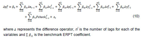 An argument against ERPT estimates based on first differences is the misspecification problem that could arise from the omission of long-run relationships that may exist (Delatte and López-Villavicencio, 2012; Aron et al., 2014). Therefore, unit root tests are performed and the long-run co-integrating relationship among the variables is estimated by employing three approaches, viz., Engle-Granger, Johansen and auto-regressive distributed lags (ARDL), with the latter approach being superior if the variables are not integrated of the same order. It also enables determination of the precise direction of causation underlying the long-run relationship.5 The error correction term (ECM) obtaining from the long-run relationship is included in (10) to avoid any systematic bias due to ignoring long-run relationships. In order to avoid any dynamic interaction of the exchange rate with the ECM, the ECM term was included with lag equal to one more than those for the maximum lag in the exchange rate terms, i.e., 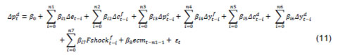 Accordingly, (11) becomes the ECM-augmented benchmark model and can be compared with (10) in order to ascertain whether or not neglect of the long-run relationship leads to serious misspecification. Based on these two alternative specifications, we examine various aspects of ERPT, viz., asymmetry in ERPT under appreciations and depreciations; non-linearity in ERPT associated with large and small exchange rate changes in either direction; and shifts in ERPT over time. II.a. Non-linearity in ERPT We examine non-linearity in ERPT in two steps. First, we fit a non-linear functional form to identify the presence of some threshold level of exchange rate changes that affects ERPT and it could differ between appreciations and depreciations. Although it is difficult to decide on a particular form a priori, we include quadratic and cubic changes in exchange rates in (10) and (11) as: The interaction of the these four dummies in (13) with (11) yields: III. Stylised Facts, Data and Results Our main interest lies in evaluating ERPT in India in the period following the global financial crisis (GFC) and comparing the results with those obtained for the pre-crisis period in which inflation was measured by wholesale prices (Khundrakpam, 2007). Two notable developments define the post-GFC years. First, this period has experienced frequent visitations of high turbulence in global financial markets on account of quantitative easing policies and announcement effects as well as geo-political tensions. Spillovers were felt in several segments of the domestic market spectrum in India, as in several other EMEs which were hostage to massive movements in risk-driven capital flows. In particular, exchange rate volatility increased on a scale not seen in the pre-GFC years right up to the ‘taper tantrum’ of the summer of 2013, followed by a period of relative tranquillity (Chart 1). The empirical literature points to a positive relationship between exchange rate volatility and ERPT – high volatility engenders greater pass-through (McCarthy, 2000; Campa and Goldberg, 2005; Jasova et al, 2016) – but only when non-linearities and time variation are accounted for. In the taper tantrum episode for instance, the Indian rupee (INR) depreciated sharply, exacerbated by weakening fundamentals and, in turn, it contributed to the persistence of high inflation. An unconventional mix of policy measures had to be resorted to stem the deterioration – forex market interventions; tightening of liquidity; restrictions on gold imports; swaps of foreign currency deposits; and macro-prudential measures. In our view, the choice of policy responses could be better informed by an accurate assessment of ERPT, taking into account asymmetries and time varying properties, rather than reactive strategies that could turn out to be inefficient and costly. 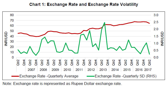 Second, the post-GFC period was characterised by high and persistent inflation by India’s own historical standards. Beginning in 2009, inflation climbed into double digits and became highly volatile on the back of a failed monsoon and a global commodity price shock. High inflation became generalised in a few months and turned persistent (Chart 2). Inflation expectations became unanchored and immune to monetary policy tightening, eventually leading up to a balance of payments crisis type situation triggered by the taper tantrum which earned India the dubious distinction of being among the ‘fragile five’ nations that were worst hit by it, as alluded to in Section I. Beginning in 2014, the RBI laid out the institutional architecture for a flexible inflation targeting framework for the conduct of monetary policy, including glide posts for headline inflation and refinements in the operating procedure. In 2016, the new monetary policy framework was made de jure by an amendment to the RBI Act by the Parliament. Importantly, the RBI adopted a new country-wide consumer price index as its metric for expressing inflation targets. Monetary policy decision making was undertaken by a committee, with failure to achieve the target and accountability clearly defined. By the second half of 2014, inflation started to gradually recede, aided in no small measure by the turning down of the commodity price cycle. Inflation volatility also moderated. These developments spurred a reawakening of interest in measuring ERPT through these tumultuous times: do changes in exchange rate and inflation volatility impact ERPT? Is ERPT stable in the face of these large movements? What are the implications for monetary policy? 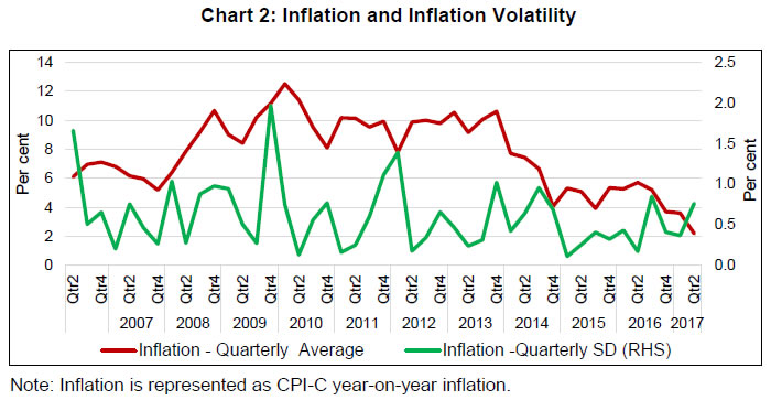 The analysis in this section covers the period April 2005 to March 2016 mainly because it encompasses the build-up to the GFC years, its onset and the years of turbulence following in its wake, but also due to non-availability of some data series such as purchasing managers’ indices (PMI) for India prior to this period. In keeping with the estimation framework set out in Section II, domestic consumer prices are measured by the combined consumer price index (CPI-C) of the Central Statistics Office (CSO), Government of India (GoI). The exchange rate is represented by the 36-country nominal effective exchange rate (NEER) series of the Reserve Bank of India (RBI). The indicator of foreign price/cost conditions is backed out of the RBI’s 36-country real effective exchange rate (REER), i.e., cf = NEER*CPI-C/REER. Domestic demand yd is proxied by the CSO’s quarterly real GDP series converted to monthly frequency by employing the proportional Denton method6 on the seasonally adjusted index of industrial production (IIP) of the CSO. Domestic costs are depicted by Markit’s input cost indicator embedded in its PMI for manufacturing (India). Foreign demand conditions (yf) are represented by the index of industrial production (IIP) for OECD countries available at OECD. Stat and commodity prices (pc) in exporting countries are proxied by West Texas Intermediate (WTI) crude oil prices taken from Bloomberg. Unless specified otherwise, all data are taken from RBI’s data warehouse, i.e., the Database on Indian Economy (DBIE). In accordance with the sequential methodological approach set out in Section II, we proceed by first seasonally adjusting all data series by the X-12 ARIMA program of the US Census Bureau. Next, lag lengths of all control variables other than the exchange rate are selected by the general-to-specific method (also known as Hendry’s approach). Only the statistically significant lags are considered while progressively removing the insignificant ones from a maximum lag length of 11 (since we are dealing with monthly data).7 The lag length of the exchange rate depicts the duration of ERPT. The choice of the lag length is based on a screening combination of the Schwarz Bayesian Criterion (SBC), the Akaike Information Criterion (AIC) and the Hannan-Quinn Criterion (HQC).8 Preference is given to SBC in the case of any divergence between criteria, since it makes an adjustment of degrees of freedom that is important in the case of small samples (Bayoumi and Darius, 2011). Generally, however, all the three criteria select the same lag length, barring the case of asymmetric and non-linear ERPT. III.a. Linear ERPT The benchmark estimate of ERPT presented in Table 1 (column 1) shows that foreign costs, domestic costs and domestic demand - which are all stationary in first differences (Table 1, APPENDIX) - are statistically significant determinants of CPI inflation in India. All the lag length selection criteria point the appropriate lag length for the exchange rate being four months. ERPT accumulated over these four months is 0.156, i.e., about 16 per cent of exchange rate changes are cumulatively passed through to CPI inflation. Co-integration tests, viz., Engle-Granger, Johansen and ARDL tests (Table 2 and 3, APPENDIX) indicate the existence of a unique long-run relationship between the CPI, the exchange rate, foreign costs and domestic costs.9.- Accordingly, the benchmark model is augmented with ECM terms obtained from the three alternative estimates of the long-run relationship alluded to earlier.10 The results reported in column (2) to (4) in Table 1 show that all the ECM terms are statistically significant, the fit of the estimates improves with their inclusion and the coefficients on control variables, viz., foreign costs, domestic costs and domestic demand increase. Importantly, ERPT remains stable at around 15 to 16 percent. III.b. Robustness of ERPT Estimates The structural impulse response function (IRF) of a unit exchange rate shock to inflation is statistically significant in the first two months. The accumulated responses work out to be -0.147 for the first two months and -0.153 at the end of 12 months indicating that ERPT is around 15 per cent (Chart 3). This is consistent with the single equation estimates. III.c. Non-Linearity in ERPT Non-linearity in ERPT is estimated by introducing quadratic and cubic exchange rate terms in (11) to gauge whether or not the size of exchange rate changes matter (Table 2). Both the quadratic and cubic terms are significant in all the four alternative models. There is also some improvement in the explanatory power relative to the linear models presented in Table 1, implying that a non-linear function fits the data better. 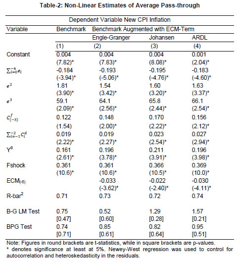 In both the benchmark models as well as in the one augmented with ECM terms, the linear function overestimates ERPT when both exchange rate depreciations and appreciations are large (Chart 4). For small changes, the slope of depreciations seems to be steeper than appreciations, implying higher ERPT from small depreciations than from small appreciations. It also appears that there are inflexion points splitting exchange rate changes around which the simultaneous play of quadratic and cubic terms leads to changes in ERPT on both sides. Consequently, separate linear functions can be employed to estimate ERPT for these sub-periods. These inflexion points are -0.022 (or 26.0 per cent on an annualised basis) for depreciation and around 0.015 (18.0 per cent on an annualised basis) for appreciation. Another inflexion point is at zero, which reinforces the asymmetry in ERPT between depreciation and appreciation.11 Next we prospect for the joint presence of asymmetry and non-linearity in ERPT by splitting appreciations and depreciations at threshold points, i.e., at -0.022 for depreciations and 0.015 for appreciations. Based on the kernel density distribution, we consider at least 25 per cent of the sample data (at least 17 data points) for large appreciations and depreciations. Accordingly, we estimate a split linear regression with three inflexion points, viz., at -0.021, 0.00 and 0.0145 (Table 3). The benchmark model suggests that ERPT from small depreciations (-0.305) and small appreciations (-0.188) is much higher than from large depreciations (-0.159) and large appreciations (-0.06). Between depreciation and appreciation, ERPT is higher for the former than for the latter for both small and large changes, consistent with the results in Table 2.  Augmenting the benchmark model with ECM terms alters the results significantly. There is an increase in the value of coefficients for large appreciations (from a statistically insignificant -0.06 to a range of -0.081 to -0.088 that is significant), for small appreciations (from -0.188 to a statistically significant range of -0.218 to - 0.265) and small depreciations (from -0.305 to a statistically significant range of -0.312 to -0.381), while the coefficient on large depreciation declines (from -0.159 to a statistically significant range of -0.103 to -0.123). There is a significant asymmetric and non-linear ERPT in India, with ERPT from small depreciations being the strongest and significantly larger than from both large appreciations and depreciations. ERPT from small appreciation is also significantly larger than from large appreciation. III.d. Time variation in ERPT Time variation in ERPT is estimated by employing time varying parameter (TVP) regressions of the equations (15) and (16) (Nakajima, 2011). Given the data set, samples are drawn from a posterior distribution following a Markov Chain Monte Carlo (MCMC) algorithm using the Matlab codes developed by Nakajima.11 Due to lack of sufficient data points, the analysis is restricted by selecting a reasonably flat prior for the initial state from the standpoint that we have no information about the initial state a priori. To compute the posterior estimates, 10,000 samples are drawn.12 The diagnostics suggest that the MCMC algorithm produces posterior draws efficiently (Chart 2 and Table 5, APPENDIX). The sample paths are stable and the sample autocorrelations are low, especially after the initial draws. The estimates of convergence diagnostics derived from the MCMC sample show that the convergence to the posterior distribution is accepted for the parameters (Geweke, 1991). The inefficiency factors were also found to be relatively low, indicating an efficient sampling procedure. The time varying ERPT plotted in Chart 5 shows substantial variations over the last decade. It can be seen that ERPT gradually increased to around 15 -20 per cent by 2013-14 followed by a declining tendency since then (Chart 5). III.e. Determinants of Time Varying ERPT In the literature, among several hypotheses offered and validated empirically in cross-country settings, an influential view is that the time varying nature of ERPT is expected to be larger in an environment of high inflation in which pricing power is stronger (Taylor, 2000). The cross-country experience has provided empirical validation (Baqueiro, de León, and Torres, 2003; Baillie and Fujii, 2004; Maria-Dolores, 2009; Junttila and Korhonen, 2012; and Ozkan and Erden, 2015). Support for this hypothesis has also emerged from the discernible anchoring of inflation expectations under inflation targeting (IT) and the associated decline in ERPT that it has brought with it (Mishkin and Savastano, 2000; Schmidt-Hebbel and Werner, 2002). However, the basic constraints on empirical assessment of this hypothesis has been short sample periods under IT and this has been sought to be overcome by employing intra-month volatility in inflation (Gagnon and Ihrig, 2004). Second, higher volatility in exchange rates is associated with higher ERPT. Large variations in exchange rates generate uncertainty and encourages importers to adjust their prices to keep their profit margins unchanged (Campa and Goldberg, 2002; and McCarthy, 2000). Third, the higher the degree of openness allows higher ERPT as global shocks are transmitted more easily to open economies through exchange rate movements (Ozkan and Erden, 2015). In order to examine the validity of these hypotheses in the Indian case, the following equation is estimated:  The results indicate that the coefficient on the inflation rate is positive and significant in both pre and post-2014 periods, validating the Taylor hypothesis. In fact, it is larger for the post-2014 period than for the earlier period. The coefficient of inflation volatility is significant at the 10 per cent level. The institution of inflation targeting framework has evidently helped in lowering both the level and volatility of inflation which could have resulted in lower ERPT, validating the priors set up earlier. The statistically significant positive coefficient on exchange rate volatility is mainly due to the fact that India’s imports are mostly invoiced in US dollars and volatility in the exchange rate imparts a shock to import prices. In the presence of menu costs, firms would pass it on to domestic prices to preserve profit margins. Increasing openness of the economy leads to higher ERPT, as indicated by the statistically significant positive coefficient on the trade to GDP ratio (Table 4). | Table 4: Determinants of Time Varying ERPT | | Dep: ERPT | Coeff. | SE | t | p-value | | π (1-D) | 0.007 | 0.004 | 1.720 | 0.093 | | π (D) | 0.021 | 0.009 | 2.280 | 0.029 | | πvol | 0.011 | 0.006 | 1.910 | 0.064 | | evol | 0.018 | 0.007 | 2.450 | 0.019 | | OPEN | 0.035 | 0.011 | 3.140 | 0.003 | | αD | 0.107 | 0.022 | 4.910 | 0.000 | | α | 0.072 | 0.011 | 6.290 | 0.000 | | Note: ERPT is represented as a positive variable by multiplying by (-1) for ease of interpretation. Newey-West regression was used to control for autocorrelation and heteroskedasticity in the residuals. | The historical variable decomposition of ERPT indicates that the increase in ERPT from around 5 per cent to above 15 per cent during 2010-2014 was largely driven by increased openness and exchange rate volatility. On the other hand, in the post-2014 period, the lowering of inflation and a fall in the trade to GDP ratio contributed significantly to the lowering of ERPT (Chart 6). IV. Policy Implications of Time Varying and Non-Linear ERPT Given the incompleteness of ERPT in India, it is useful to examine the monetary policy implications of our results within a small macro-economic model. Belonging in the new Keynesian tradition, it preserves tractability within the rigour of a dynamic optimising general equilibrium form (Monacelli, 2005). The incompleteness of ERPT essentially represents a deviation from the law of one price. Therefore, in contrast to the canonical models in this stream which assume perfect ERPT (see Clarida et al., 2001, Galí and Monacelli, 2005), we evaluate the range of estimates of incomplete and time-varying ERPT obtained in Section III by calibrating an open-economy DSGE model (Monacelli, 2005) for the Indian economy13 under three different types of shocks, viz., a monetary policy shock conveyed through the policy interest rate; a foreign inflation shock; and a domestic productivity or positive supply shock. Drawing heavily on Monacelli (2005), we set out the four equations that form the backbone of the model below (see Table 6, APPENDIX for the full set of log-linearised equations). Inflation in imported goods and services is represented by the following equation: 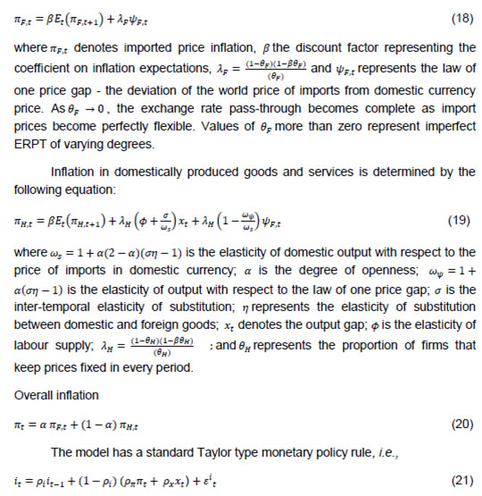 We calibrate the model using parameters derived from several relevant studies in the Indian context (Levine, et al., 2012; Ghate, 2016; Anand and Prasad, 2010; and Patra and Kapur, 2012) (Table 7, APPENDIX). Essentially, we generate the impulse response functions (IRFs) of a contractionary monetary policy shock, a positive shock to the inflation in rest of the world and a positive domestic productivity shock under different values of θF, i.e., different degrees of ERPT (Chart 5). The simulations are carried out for values of θF ranging from 0.10 to 0.95, encompassing the different degrees of ERPT that have been estimated in Section III under alternative combinations of asymmetry, non-linearity and time variation. As ERPT increases from 0.02 to 0.38 the value of θF decreases from 0.95 to 0.10.14 The basic idea is to analyse how the impulse response of a particular shock is influenced by the degree of ERPT. Consequently, monetary policy responses may have to be different. The top panel of Chart 5 (a and b) represents the response of the output gap and inflation to a one standard deviation contractionary shock from the policy rate under different values of θF. While the size of ERPT has very little influence on the responsiveness of the output gap to the policy rate shock, the responsiveness of inflation is highly sensitive to it. Furthermore, the sacrifice ratio – defined as the cumulative output loss for a unit of disinflation – is highly sensitive to the size of ERPT. When ERPT is low at about 0.02 (θF = 0.95), the sacrifice ratio is high at around 3.67, while for higher ERPT of 0.38 (θF = 0.10) the sacrifice ratio is markedly lower at about 1.74 (Chart 5.c). Higher ERPT strengthens the exchange rate channel of monetary policy transmission. A tightening of monetary policy induces domestic currency appreciation and reduces inflation faster than otherwise. Consequently, a unit disinflation can be achieved with a much lower loss of output under higher ERPT than under lower ERPT. In the context of our estimates of ERPT non-linearities, the effectiveness of monetary policy on inflation would also be conditioned by the size and the direction of the exchange rate change. For instance, as ERPT is higher for small depreciations than for large ones (more than three times), monetary policy tightening would be more effective in reducing inflation with less output loss during a phase of small currency depreciations relative to large depreciations. The response of inflation, its imported component and the policy rate to a one standard deviation positive shock to foreign inflation is sharper when ERPT is higher (second panel of Chart 5- d to e). Consequently, a larger monetary policy response would be warranted (Chart 5.f). The policy implication in the context of our ERPT estimates is that the transmission of foreign shocks would be much stronger during periods of small exchange rate movements because they are associated with higher ERPT. In contrast, the responses of the output gap, inflation and monetary policy to a one standard deviation productivity (supply) shock are muted and, in fact, are hardly affected by the size of ERPT (Chart 5.g to i). V. Conclusion The degree of ERPT matters for the conduct of monetary policy, and particularly so in a flexible inflation targeting framework, as it informs the policy maker about the extent to which the goal variable – the domestic inflation – is hostage to imported influences. Invariably it conditions the decision on the direction and size of instrument variable adjustment. For the policy maker, therefore, precision is key in what is ultimately an empirical issue. As against the received wisdom that ERPT is low in AEs and declining in EMEs derived by estimating it as a linear and symmetric process, this paper explores non-linear, asymmetric and time varying properties of ERPT in the Indian context. In doing so, it contributes country-specific evidence to the animated debate on the theme, which becomes interesting in the context of the changing inflation dynamics in India in recent years in an environment of high volatility in food price due to supply shocks and exchange rate volatility stirred up by bouts of global financial market turbulence. The adoption of flexible inflation targeting as the framework for monetary policy influences the discussion significantly. Important policy inputs are offered. Notably, the degree of ERPT has declined in the post-2014 period than in the years prior to it. This expands the degrees of freedom for the policy maker in India to pursue independent monetary policy. ERPT matters, i.e., about 15 per cent of exchange rate changes are cumulatively passed through to CPI inflation over a period of five months, with time varying parameter estimation increasing it to above 15 per cent by 2013-14 and declining since then. With 80 per cent of the national requirement of the petroleum products imported along with almost all of domestic gold consumption, this is critical information – on an average a one percent change in the exchange rate translates to 15 bps change in headline inflation. 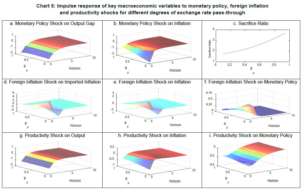 Moreover, a hierarchy of monetary policy responses can be calibrated to the degree of ERPT – small depreciations; large depreciations; small appreciations; and large appreciations; in that order. For instance, in the context of monetary policy engaged in disinflation, the policy rate needs to be raised less aggressively during small depreciations than in the case of large appreciations, assuming the absence of foreign inflation shocks. The intrepid policy maker is best served by a reasonable fix on hierarchical magnitudes so as to calibrate policy actions as needed. In sum, the effectiveness of monetary policy in India is influenced by the size and direction of exchange rate movements which, in turn, affect the responses of the output gap and inflation to monetary policy and foreign inflation shocks. While a larger ERPT enhances monetary policy transmission by strengthening the exchange rate channel of monetary policy transmission, it also poses significant challenges in terms of managing imported inflation. Monetary policy transmission is likely to be stronger during periods of small depreciations when ERPT is estimated to be the strongest, but the transmission of the same shock to domestic inflation would be strong too. The dilemma just got sharper.
References Anand, R., & Prasad, E. S. (2010). Optimal price indices for targeting inflation under incomplete markets (No. w16290). National Bureau of Economic Research. Aron, J., Macdonald, R., & Muellbauer, J. (2014). Exchange rate pass-through in developing and emerging markets: A survey of conceptual, methodological and policy issues, and selected empirical findings. Journal of Development Studies, 50(1), 101-143. Aron, J., Creamer, K., Muellbauer, J., & Rankin, N. (2014). Exchange rate pass-through to consumer prices in South Africa: Evidence from micro-data. Journal of Development Studies, 50(1), 165-185. Aron, J., Farrell, G., Muellbauer, J., & Sinclair, P. (2014). Exchange rate pass-through to import prices, and monetary policy in South Africa. Journal of Development Studies, 50(1), 144-164. Bailliu, J., & Fujii, E. (2004) Exchange Rate Pass-Through and the Inflation Environment in Industrialized Countries: An Empirical Investigation, Bank of Canada working paper no. 21. Baqueiro, A., De Leon, A. D., & Torres, A. (2003). Fear of floating or fear of inflation? The role of the exchange rate pass-through. BIS papers, (19), 338-354. Bayoumi, T., & Darius, R. (2011). Reversing the Financial Accelerator; Credit Conditions and Macro-Financial Linkages (No. 11/26). International Monetary Fund. Borio, C., & Disyatat, P. (2010). Unconventional monetary policies: an appraisal. The Manchester School, 78(s1), 53-89. Bussiere, M. (2013). Exchange Rate Pass‐through to Trade Prices: The Role of Nonlinearities and Asymmetries. Oxford Bulletin of Economics and Statistics, 75(5), 731-758. Calvo, G. A., & Reinhart, C. M. (2000). Fixing for Your Life. In Brookings Trade Forum (pp. 39-54). Calvo, G. A., & Reinhart, C. M. (2002). Fear of floating. The Quarterly Journal of Economics, 117(2), 379-408. Campa, J. M., & Goldberg, L. S. (2005). Exchange rate pass-through into import prices. Review of Economics and Statistics, 87(4), 679-690. Cheikh, B. N., & Rault, C. (2016). The Pass‐through of Exchange Rate in the Context of the European Sovereign Debt Crisis. International Journal of Finance & Economics, 21(2), 154-166. Clarida, R., Gali, J., & Gertler, M. (2001). Optimal monetary policy in open versus closed economies: an integrated approach. The American Economic Review, 91(2), 248-252. Delatte, A. L., & López-Villavicencio, A. (2012). Asymmetric exchange rate pass-through: Evidence from major countries. Journal of Macroeconomics, 34(3), 833-844. Devereux, M. B., & Yetman, J. (2010). Price adjustment and exchange rate pass-through. Journal of International Money and Finance, 29(1), 181-200. Franta, M., Horvath, R., & Rusnak, M. (2014). Evaluating changes in the monetary transmission mechanism in the Czech Republic. Empirical Economics, 46(3), 827-842. Gabriel, V., Levine, P., Pearlman, J., & Yang, B. (2010). An estimated DSGE model of the Indian economy. NIPE WP, 29, 2010. Gagnon, J. E., & Ihrig, J. (2004). Monetary policy and exchange rate pass‐through. International Journal of Finance & Economics, 9(4), 315-338. Gali, J., & Monacelli, T. (2005). Monetary policy and exchange rate volatility in a small open economy. The Review of Economic Studies, 72(3), 707-734. Geweke, J. (1991). Evaluating the accuracy of sampling-based approaches to the calculation of posterior moments (Vol. 196). Minneapolis, MN, USA: Federal Reserve Bank of Minneapolis, Research Department. Ghate, C., Gupta, S., & Mallick, D. (2016). Terms of Trade Shocks and Monetary Policy in India. Computational Economics, 1-47. Goldberg, L. S., & Campa, J. M. (2010). The sensitivity of the CPI to exchange rates: Distribution margins, imported inputs, and trade exposure. The Review of Economics and Statistics, 92(2), 392-407. Goldberg, P. K., & Hellerstein, R. (2008). A structural approach to explaining incomplete exchange-rate pass-through and pricing-to-market. The American Economic Review, 98(2), 423-429. Hara, N., Hiraki, K., & Ichise, Y. (2015). Changing exchange rate pass-through in Japan: does it indicate changing pricing behavior? (No. 15-E-4). Bank of Japan. Jašová, M., Moessner, R., & Takáts, E. (2016). Exchange rate pass-through: What has changed since the crisis? (No. 583). Bank for International Settlements. John, J. (2015). Has Inflation Persistence In India Changed Over Time?. The Singapore Economic Review, 60(4), 1-16. Jooste, C., & Jhaveri, Y. (2014). The Determinants of Time‐Varying Exchange Rate Pass‐Through in South Africa. South African Journal of Economics, 82(4), 603-615. Junttila, J., & Korhonen, M. (2012). The role of inflation regime in the exchange rate pass-through to import prices. International Review of Economics & Finance, 24, 88-96. Kapur, M., & Patra, M. D. (2012). Alternative Monetary Policy Rules for India IMF Working Paper No. 12/118. International Monetary Fund. Khundrakpam, J. (2007). Economic reforms and exchange rate pass-through to domestic prices in India (No. 225). Bank for International Settlements. Knetter, M. M. (1994). Is export price adjustment asymmetric?: Evaluating the market share and marketing bottlenecks hypotheses. Journal of International Money and Finance, 13(1), 55-70. Lopez-Villavicencio, A., & Mignon, V. (2016). Exchange rate pass-through in emerging countries: Do the inflation environment, monetary policy regime and institutional quality matter? (No. 2016-18). University of Paris West-Nanterre la Défense, EconomiX. María-Dolores, R. (2009). Exchange Rate Pass-Through in Central and East European Countries: Do Inflation and Openness Matter?. Eastern European Economics, 47(4), 42-61. McCarthy, J. (2007). Pass-Through of Exchange Rates and Import Prices to Domestic Inflation in Some Industrialized Economies. Eastern Economic Journal, 33(4), 511-537. McFarlane, L. (2009). Time-varying exchange rate pass-through: An examination of four emerging market economies. Bank of Jamaica. Available at http://www.cemla.org/red/papers2009/JAMAICA-McFarlane.pdf. Mihaljek, D., & Klau, M. (2008). Exchange rate pass-through in emerging market economies: what has changed and why?. BIS Papers, 35, 103-130. Mishkin, F. S., & Savastano, M. A. (2001). Monetary policy strategies for Latin America. Journal of Development Economics, 66(2), 415-444. Monacelli, T. (2005). Monetary Policy in a Low Pass-through Environment. Journal of Money, Credit & Banking, 37(6), 1047-1067. Mumtaz, H., & Sunder‐Plassmann, L. (2013). Time‐Varying Dynamics of the Real Exchange Rate: An Empirical Analysis. Journal of Applied Econometrics, 28(3), 498-525. Nakajima, J. (2011). Monetary Policy Transmission under Zero Interest Rates: An Extended Time-Varying Parameter Vector Autoregression Approach. The BE Journal of Macroeconomics, 11(1), 1-24. Obstfeld, M., & Rogoff, K. (2000). The six major puzzles in international macroeconomics: is there a common cause?. NBER macroeconomics annual, 15, 339-390. Ozkan, I., & Erden, L. (2015). Time-varying nature and macroeconomic determinants of exchange rate pass-through. International Review of Economics & Finance, 38, 56-66. Patra, M. D., & Kapur, M. (2012). A monetary policy model for India. Macroeconomics and Finance in Emerging Market Economies, 5(1), 18-41. Patra, M. D., Khundrakpam, J. K., & George, A. T. (2014, August). Post-Global Crisis Inflation Dynamics in India: What has Changed?. In India Policy Forum (Vol. 10, No. 1, pp. 117-203). National Council of Applied Economic Research. Pollard, P. S., & Coughlin, C. C. (2003). Size Matters: Asymmetric Exchange Rate Pass-Through At The Industry Level. Federal Reserve Bank of St. Louis Working Paper Series, (2003-029). Schmidt-Hebbel, K., Werner, A., Hausmann, R., & Chang, R. (2002). Inflation Targeting in Brazil, Chile, and Mexico: Performance, Credibility, and the Exchange Rate [with Comments]. Economia, 2(2), 31-89. RBI (2014). Report of the Expert Committee to Revise and Strengthen the Monetary Policy Framework. Available at https://rbidocs.rbi.org.in/rdocs/PublicationReport/Pdfs/ECOMRF210114_F.pdf. Shioji, E. (2014). A Pass‐Through Revival. Asian Economic Policy Review, 9(1), 120-138. Shioji, E. (2015). Time varying pass-through: Will the yen depreciation help Japan hit the inflation target? Journal of the Japanese and International Economies, 37, 43-58. Taylor, B. J. (2000). Low inflation, pass-through and the pricing power of firms, European Economic Review, 44(7), pp 1389–1408. Webber, A. (2000). Newton’s gravity law and import prices in the Asia Pacific, Japan and the World Economy 12(1), pp 71–87.
APPENDIX | APPENDIX Table 1: Unit Root Tests | | Variable (X) | ADF | Phillips-Perron | | | Log X | ΔLog X | Log X | ΔLog X | | Pd | -0.24 | -9.57* | -0.24 | -9.57* | | e | -2.40(t) | -9.03* | -2.09(t) | -9.01* | | Yd | -2.98(t) | -3.58* | -2.46(t) | -3.09** | | Yw | -2.22(t) | -3.79* | -0.76 | -3.06** | | Cd | -3.19** | -11.8* | -3.25** | 12.5* | | Cf | -1.88(t) | 12.2* | 1.92(t) | -12.2* | | Fshock | | -6.88* | | -11.7* | | Pc | -1.88 | -8.87* | -1.75(t) | -8.97* | | Notes: * and ** denote significance at 1 and 5 per cent level, respectively. The lag length in the ADF tests was chosen based on Schwarz Bayesian Criterion (SBC). ‘t’ in the parentheses indicate inclusion of a trend component in the estimates, which was based on its statistical significance in the equation. |
| APPENDIX Table 2: Bounds Test for Cointegration | | Variables | F-Statistic | W-Statistic | Cointegration | | FY(logPd/logCd, loge,logCf) | 6.08* | 24.33* | Accepted | | FY(logCd/ logPd, loge,logCf) | 2.75 | 10.99 | Rejected | | FY(loge/logCd,logPd,logCf) | 1.40 | 5.60 | Rejected | | FY(logCf/loge,logCd,logPd) | 2.81 | 11.23 | Rejected | | Notes: The 95% upper critical bound values for F-statistics and W-statistic, respectively, are 4.44 and 17.75. |
APPENDIX Table 3: Estimated Long-run Relationships
(dependent variable logPd) | | Variables | ARDL | Engle-Granger | Johansen | | Constant | -2.83
(-3.00)* | -2.28
(-5.56)* | -2.40
(n.a.) | | logCd | 0.254
(4.01)* | 0.088
(3.60)* | 0.264
(4.99)* | | Loge | -0.408
(-4.17)* | -0.396
(-9.25)* | -0.474
(-5.32)* | | logCf | 1.81
(16.9)* | 1.80
(39.1)* | 1.75
(18.3)* | | Notes: * and ** denote significance at 1% and 5% level, respectively. Both ADF and Phillips-Perron tests show the residual of the long-run estimate under Engle-Granger test is stationary. Using Johansen’s method, both the trace and eigen value tests show one co-integrating relationship. |
| APPENDIX Table 4: Lagrange-multiplier test – SVAR | | Lag | chi2 | df | p-value | | 5 | 11.90 | 9 | 0.219 | | 6 | 10.69 | 9 | 0.297 | | 7 | 9.12 | 9 | 0.426 | | 8 | 7.88 | 9 | 0.547 | | 9 | 16.29 | 9 | 0.061 | | 10 | 8.27 | 9 | 0.507 | | 11 | 3.33 | 9 | 0.950 | | 12 | 15.57 | 9 | 0.077 |
| APPENDIX Table 5: Estimation results of hyper parameters in the TVP Regression model | | Parameter | Mean | Stdev | 95%U | 95%L | Geweke | Inefficiency | | Sig11 | 0.218 | 0.146 | 0.058 | 0.609 | 0.111 | 30.170 | | Sig22 | 0.192 | 0.132 | 0.052 | 0.533 | 0.160 | 32.950 | | Sig33 | 0.103 | 0.067 | 0.030 | 0.272 | 0.055 | 40.510 | | Sig44 | 0.051 | 0.029 | 0.015 | 0.129 | 0.064 | 40.990 | | Sig55 | 0.027 | 0.016 | 0.009 | 0.067 | 0.106 | 37.720 | | Sig66 | 0.014 | 0.007 | 0.005 | 0.032 | 0.205 | 31.030 | | Sig77 | 0.008 | 0.003 | 0.003 | 0.016 | 0.239 | 12.870 | | Sig88 | 0.005 | 0.002 | 0.002 | 0.010 | 0.188 | 11.710 | | Sig99 | 0.003 | 0.001 | 0.002 | 0.006 | 0.789 | 7.530 | | Sig00 | 0.002 | 0.001 | 0.001 | 0.004 | 0.279 | 7.390 | | Sig11 | 0.002 | 0.001 | 0.001 | 0.003 | 0.807 | 8.300 | | sigma | 1.739 | 1.077 | 0.439 | 4.467 | 0.111 | 1.610 | | Note: To check the convergence of the MCMC, as suggested by Geweke (1991), the p-value of difference in average between the first n0 draws and the last n1 draws is reported. The inefficiency factor is computed to measure how well the MCMC chain mixes. It is function of sample autocorrelation at various lags. |
| APPENDIX Table 7: Calibration of key parameters in the DSGE Model for India | | Parameter | Description | Value | Calibration | | σ | Inter-temporal elasticity of consumption | 1.99 | Levine, et al. (2012) and Ghate (2016) | | α | Degree of openness of domestic economy | 0.42 | Trade as volume of GDP (10 year average) | | η | Elasticity of substitution between domestic and foreign goods | 1.0 | Kletzer and Ghate (2016) | | ϕ | The inverse of elasticity of labor supply in CES utility function | 3.0 | Anand and Prasad (2010) and Ghate (2016) | | β | Temporal discount factor | 0.9823 | Levine, et al. (2012) and Ghate (2016) | | ρπ | Inflation coefficient in Taylor rule | 1.1 | Patra and Kapur (2012) | | ρx | Output gap coefficient in Taylor rule | 0.4 | Patra and Kapur (2012) | | ρi | Interest rate smoothing | 0.8 | Estimated AR(1) | | θH | Domestic producers Calvo probability - Measure of sickness - | 0.75 | Levine, et al. (2012) and Ghate (2016) | | θF | Import pricing Calvo probability | 0.75 | Assumed to be similar as domestic | |