Press Release RBI Working Paper Series No. 08
Phillips Curve Relationship in India:
Evidence from State-Level Analysis @Harendra Behera
Garima Wahi
and
Muneesh Kapur Abstract 1This paper revisits the issue of determinants of inflation in India in a Phillips curve framework and makes two key contributions in relation to existing studies. First, in the context of the Reserve Bank moving towards a flexible inflation targeting framework based on consumer price index (CPI) inflation, this paper attempts to model dynamics of the CPI inflation. Second, this paper explores the Phillips curve relationship using sub-national data in a panel-approach. The estimates in this paper confirm the presence of a conventional Phillips curve specification, both for core inflation and headline inflation. Excess demand conditions have the expected hardening effect on inflation, with the impact being more on core inflation. Exchange rate movements are also found to have a significant impact on inflation. Overall, the paper’s findings provide support for the role of a counter-cyclical monetary policy to stabilise inflation and inflation expectations. JEL classification: E31, E32, E52, E58 Keywords: Consumer Price Inflation, Exchange Rate Pass-through, Monetary Policy, Phillips Curve. Introduction A forward-looking assessment of inflation is a critical input for an effective conduct and formulation of monetary policy. The Phillips curve framework relating inflation to economic activity and other determinants such as exchange rate has been used extensively to explore this relationship both in India and across countries. In India, the focus of most of the Phillips curve studies has been on wholesale price index (WPI) as an indicator of inflation. With the move towards consumer price index-combined (CPI-C) based flexible inflation targeting beginning 2014, determinants of CPI inflation and its forecasts assume critical importance (RBI, 2014a; RBI, 2016). A key objective of this paper is, therefore, to understand the drivers of CPI inflation in a more robust framework. While some studies have modelled the inflation process for CPI for industrial workers (CPI-IW) and back-casted CPI-C, we are not aware of any study on the CPI-C inflation process per se. As the dynamics of these two price indices could be different, this paper, therefore, models both the CPI-IW and the CPI-C inflation processes and attempts to draw policy implications. The focus of the Phillips curve studies has typically been on the national level relationship, both in the Indian and the cross-country context. More recently, a number of studies have attempted to assess this relationship using the sub-national level data for a variety of reasons. First, the relatively more variability at sub-national levels in both inflation and output indicators, as also more data points, provide a rationale for examining this relationship using the sub-national level data. Second, a possible weakening of the inflation-output relationship at the national level could arise if the central bank is successful in keeping the national inflation close to its target; in such a scenario, swings in economic activity (above or below potential) may be only weakly associated with movements in the national level inflation, thereby weakening the inflation-output nexus. At the same time, the continued dispersion in sub-national data on inflation – not the central bank’s target per se - can still provide the researchers an avenue to explore the inflation-output dynamics. While such sub-national level studies have been undertaken in the context of the US and few other countries, such an endeavour has not been attempted in the Indian context. Against this backdrop, this paper empirically assesses the Phillips curve relationship for CPI inflation (CPI-IW as well as CPI-C) in India using state-level data in a panel framework. The structure of the paper is as follows: this introductory section is followed (Section II) by a brief review of the literature on the Phillips curve studies. A discussion of empirical methodology, and data sources and properties are in Section III. Empirical results across various specifications are presented and analysed in Section IV, with concluding observations in Section V. II. Phillips Curve Framework: A Review The Phillips curve framework relating inflation to economic activity continues to be the workhorse model for understanding inflation dynamics, even as it has faced a number of challenges in the past and is confronted with new complexities in the aftermath of the Great Recession (Stock and Watson, 2009). Inflation in the major advanced economies has deviated persistently from forecasts from the conventional Phillips curve specifications since 2008: actual inflation during 2009-2010 was higher than expected, while in the more recent period, especially in the US, inflation has turned out to be lower than expected. The years 2009 and 2010 were marked by the phenomenon of “missing deflation” in the US and other major advanced economies: given the large negative unemployment and output gaps, the Phillips curve framework would have predicted a sharp decline in inflation (or, even outright deflation), whereas the actual core inflation was close to its 2008 level (Ball and Mazumder, 2015). On the other hand, with the unemployment rate falling below 5 per cent in the US by 2016, close to or below its natural rate, an emergence of inflationary pressures was expected, but inflation has actually turned out to be quiescent. Although the “US Phillips curve is alive and well (or at least as well as it has been in the past)”, its inability to fully explain inflation dynamics as well as its flattening “raises serious challenges for monetary policy in the future” (Blanchard, 2016a; pp. 31 and 34). A number of alternative explanations have been offered for the missing deflation/inflation phenomenon: well-anchored inflation expectations and a flattening of the Phillips curve (Blanchard et al., 2015); the short-term unemployment rate (which has exhibited significantly lower decline than the overall unemployment rate) matters more for inflation than the overall unemployment rate (Ball and Mazumder, 2015); the inflation expectations of households (which are more volatile and elevated) matter and not the relatively stable expectations of financial markets (Coibion and Gorodnichenko, 2015); the Phillips curve might be convex, with the response of inflation to demand conditions being quite muted during recessions vis-à-vis expansions (Gross and Semmler, 2017); and, not only domestic but global factors need to be factored in appropriately (Bobeica and Jarocinski, 2017). The Phillips curve specifications, therefore, appear to remain appropriate in explaining the recent inflation dynamics. There is some evidence of a flattening of the Phillips curve in advanced economies along with an improved anchoring of inflation expectations. For example, Blanchard et al. (2015) find that the median coefficient of unemployment gap fell from over unity in the mid-1970s to around 0.2-0.3 in the early 1990s and has remained around that level since then. While the median coefficient in their sample countries during the 2000s is statistically significant, the individual coefficients for most countries (including the major ones such as the US and Germany) are small and statistically insignificant, although their results are sensitive to the methodology. The flattening of the Phillips curve has important policy implications: “to the extent that the unemployment gap has a smaller effect on inflation, monetary policy rules should put relatively more weight on the unemployment gap relative to inflation. Trying to stabilize inflation may require very large movements in the unemployment gap” (Blanchard et al., 2015). The observed flattening of the Phillips curve could indeed be due to anchored inflation expectations as argued by Blanchard et al. (2015), but it could also be due to the inability of the national level data to appropriately capture inflation-demand nexus for a variety of reasons. First, if the central bank targets national inflation and is broadly successful in keeping inflation (especially core inflation) as well as inflation expectations close to the target, then a corollary of this is that the relationship between national inflation and output might weaken or, in an extreme case, there might be no relationship at all (Fitzgerald et al., 2013). At the same time, since the sub-national level inflation rates are not the central bank’s target per se, one can expect substantial variation in inflation rates across regions/states. Similarly, the national level output gap might be positive (or negative), even as some of the regions might be witnessing a negative output gap (and vice versa). This heterogeneity in local inflation rates and local demand conditions can then be used to exploit and study the inflation-output relationship. On the other hand, high labour mobility across regions within a country could be expected to weaken the regional inflation-output relationship (Coen et al., 1999). Second, some of the recently advanced hypothesis – such as the relative role of the short-term and long-term unemployment rates – to explain the inflation dynamics cannot be convincingly explained through the national level data, given the strong historical co-movement between the short- and long-term unemployment rates (Kiley, 2015). Again, the state-level data, with its heterogeneity, can be more fruitfully used to assess alternative hypothesis (such as linearity or non-linearity of the Phillips curve). Turning to the empirical evidence from the studies based on the sub-national data, Wall and Zoega (2003) find that more cross-state dispersion of unemployment rates and employment growth means a higher level of aggregate wage inflation even if aggregate unemployment and employment growth are unchanged. Kumar and Orrenius (2016) find strong evidence of non-linearity and convexity in the wage-price Phillips curve in the US in contrast to the mixed evidence from the national data; declines in the unemployment rate below the average unemployment rate exert significantly higher wage pressure than changes in the unemployment rate above the historical average. On the issue of short- versus long-term unemployment rates, Smith (2014) and Kiley (2015) are unable to find any differential impact of short- and long-term unemployment rates on wage/price inflation in the US. On the other hand, Kumar and Orrenius (2016) find that the short-term unemployment rate has a strong relationship with both average and median wage growth, while the long-term unemployment rate appears to influence only median wage growth2. Aaronson and Sullivan (2000) and Fitzgerald et al. (2013) find that the Phillips curve exhibits stability when regional data are used, but the relationship weakens or turns unstable when national level data are used, corroborating the view that the successful pursuit of a national inflation target by the central bank may break or weaken the aggregate relationship. On the other hand, Osadcha (2014) finds support for both national and state-level Phillips curve. Mehrotra et al. (2007) examine drivers of provincial inflation in China in a hybrid New Keynesian Phillips Curve (NKPC) framework and find the NKPC can explain the inflation process for coastal states only, attributable to these states being more market-oriented and relatively more demand pressures. Empirical Evidence: India In the Indian context, a number of studies have found support for the Phillips curve framework at the national level, with inflation (measured by movements in WPI) responding both to demand and supply shocks. These include Kapur and Patra (2000), RBI (2002, 2004), Dua and Gaur (2009), Paul (2009), Patra and Ray (2010), Singh et al. (2011), Mazumder (2011), Patra and Kapur (2012), and Kapur (2013). Srinivasan et al. (2006), on the other hand, could not find support for the Phillips curve. A comprehensive review of these studies and updated estimates in Kapur (2013) indicates: (a) demand conditions have a relatively stronger impact on core inflation (measured by non-food manufactured products WPI inflation) vis-a-vis headline WPI inflation; (b) core inflation is more persistent than headline inflation; (c) the exchange rate pass-through coefficient is relatively modest, although large and sharp depreciation could add to inflationary pressures. This section, further reviews some subsequent studies, with particular emphasis on studies based on CPI inflation. Patra et al. (2014) explore the sources of inflation persistence in India in the NKPC framework and find: (a) supply side shocks in the form of relative price increases, particularly for food, influence aggregate prices lastingly; (b) an increase in inflation persistence in the post-2008 period; and, (c) a high degree of interest rate smoothing could be imparting persistence to the inflation process. Goyal and Tripathi (2015) find that the estimated slope of the Phillips curve is sensitive to the method of estimation and to the measurement of the supply shocks and the output gap variable. Better measurement of the supply shocks and the output gap variables reduces the size of the coefficient on the output gap. Sonna et al. (2014) examine the drivers of food inflation and find: (a) higher real rural wages as the most dominant driver; (b) the minimum support prices (MSP) policy and the changing dietary habits in favour of protein items, although statistically significant, are not as over-bearing as generally perceived; and, (c) the introduction of Mahatma Gandhi National Rural Employment Guarantee Act (MGNREGA) did not cause any significant increase in food inflation. Moving to CPI inflation based specifications, a few studies are now available, typically using CPI-IW, but their approaches and results raise some concerns. First, the preferred specification of Sen Gupta and Sengupta (2016) indicates an exchange rate pass-through of as high as 0.40 (i.e., a 10 per cent depreciation of the domestic currency could increase CPI inflation by 4 percentage points). Moreover, they estimate a fuel-price pass-through of almost 0.7 (i.e., a 10 per cent increase in fuel prices could increase CPI inflation by 7 percentage points), suggesting a very high second-order effect3. While the fuel group has a weight of 6.4 per cent in the overall CPI-IW index, the authors’ estimate of the pass-through suggests an impact equivalent to a weight of 70 per cent in the basket. Second, in Chinoy et al. (2016), the short-run estimates of the coefficient on output gap (0.52) and exchange rate (0.08) appear to be reasonable and consistent with WPI-inflation based studies, but in view of the very high persistence coefficient (the lagged inflation coefficients sum to 0.8), the long-run estimates suggest very high impact of demand conditions and exchange rate movements: a one per cent higher output gap could increase inflation by 2.6 per cent, while 10 per cent currency depreciation could lead to an increase of 4 percentage points in CPI inflation over time. Third, Chowdhury and Sarkar (2016) estimate hybrid NKPC for India (and Brazil, China and Russia) for CPI inflation, and the coefficient on output gap turns out to be perverse [negative and (in one sub-sample) statistically significant], i.e., their analysis suggests that higher demand leads to lower inflation. In Abbas (2017), the coefficient on output gap is negative and statistically significant in some specifications. While no available study directly assesses the inflation-output process at the state-level in the Indian context, a couple of studies undertake related research. First, Mohaddes and Raissi (2014) analyse state-level inflation and output in the context of examining threshold inflation. Their objective was to assess the impact of inflation on growth in the long-run (which they found to be negative), whereas our interest is the opposite: an assessment of the impact of demand conditions on inflation. Second, Goyal and Baikar (2014) attempted to model rural wage inflation and rural consumer inflation at the state-level, but their focus was mainly on the feedback between these two inflation indicators. Critically, they were unable to find any significant role for the key macroeconomic variables: activity variable (proxied by growth in index of industrial production) and the exchange rate. The lack of evidence for the activity variable could be reflecting the paper’s use of industrial production (which is less than a fifth of overall economic activity) and/or the use of growth rate (rather than in gap form); moreover, the specifications seem to be over-determined, as these also include changes in interest rate, WPI food inflation and CPI inflation as explanatory variables. Overall, as this section shows, there is strong support for the Phillips curve relationship in the Indian context. One limitation of the most available studies is their focus on WPI inflation. Moreover, the few available studies with regard to consumer price inflation are restricted either to CPI-IW or a back-casted CPI-C (using CPI-IW data for back-casting). We are not aware of any study dwelling purely on CPI-C, given the limited data availability (the CPI-C index is available from 2010 onwards, with the inflation rate being available from 2011 onwards). The challenges from the limited data span availability can be effectively addressed by recourse to an analysis using the sub-national data, an approach followed in this paper. III. Methodology and Data
We estimate these equations with random effects (as Hausman test preferred it over the fixed effects specification) and with panel-corrected standard errors (PCSE). In each case, we also report a simple Phillips curve specification, where inflation is just a function of output gap (i.e., without any controls for supply shocks). A key empirical regularity of inflation is its persistence, indicative of adaptive expectations. We, therefore, augment the baseline specifications with lagged inflation. The resultant dynamic specifications (3 and 4) are estimated through difference and system generalised method of moments (GMM) approaches of Arellano-Bond-Bover (Arellano and Bond, 1991; Arellano and Bover, 1995; and Blundell and Bond, 1998; Bond, 2002): Data The data on the CPI-Combined (CPI-C) index are available from 2010 onwards (consequently, inflation rates are available from 2011 onwards). As the limited data span with regard to CPI-C can be a concern, the paper presents results for both CPI-IW (for which longer data series are available) and CPI-C for robustness purposes. For the CPI-C series, state-wise data are provided by the Central Statistics Office (CSO). As regards the CPI-IW, the Labour Bureau provides only city-wise data; we compile state-wise CPI-IW data as a weighted average of the centre-wise indices (with weights being the centre-specific consumption expenditures of the targeted industrial workers based on Working Class Family Income and Expenditure Survey (Government of India, 2008; conducted during 1999-2000). Data on the CPI-IW series (base: 2001=100) are available from 2006 onwards and we, therefore restrict our sample to the period beginning 2006. A preliminary look at the data indicates substantial heterogeneity in both the CPI-C and CPI-IW inflation rates across Indian states (Chart 1) and this inter-state heterogeneity can be exploited for a robust analysis of the determinants of the inflation process in India. 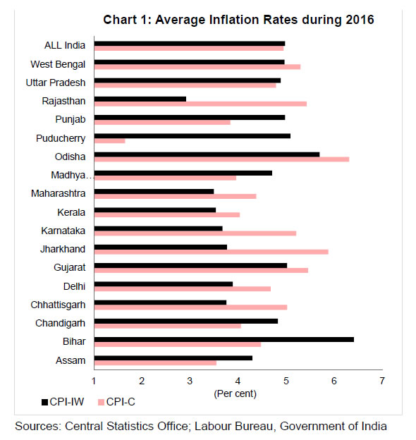 The output gap is computed as log difference of real gross state domestic product (GSDP) and its Hodrick-Prescott (HP) filtered series (multiplied by 100 to get output gap in percentage terms). Given the sensitivity of the HP filter to sample end points and also to capture the business cycle properties, output gaps are computed for the GSDP data starting 1980-814. Owing to the availability of the GSDP data on an annual basis, the paper uses data for the other variables on an annual basis as well. Rainfall data (actual rainfall less its long-period average) of each state are computed as a weighted average of the subdivision-level data (with weights being the gross cropped area of each subdivision). Apart from these state-specific variables, a few macro variables are used in the panel estimates. Exchange rate is measured by rupees per US dollar (an increase in the exchange rate denotes depreciation of the rupee, and a decline denotes appreciation). Cross-currency movements can, at times, lead to quite different trends in nominal effective exchange rates (NEER): for example, the Indian rupee depreciated by almost 5 per cent vis-à-vis the US dollar during 2015, whereas it appreciated by 2-3 per cent in NEER terms (Chart 2)5. Such large divergence in alternative indicators of the exchange rate can have significant impact on estimates – indeed, our empirical results in the next section suggest so. We, therefore, analyse results for both the rupee-dollar rate and the 36-currency trade-weighted NEER (neer36)6. Oil prices refer to international crude oil prices, measured in US dollar terms. Minimum support prices are taken as a weighted average of the prices of wheat, rice, tur, gram, urad, moong and coarse cereals (with weights being their respective shares in the CPI basket). Inflation rates and variation in other series (MSP, oil prices and exchange rate) are calculated as log-differences (and multiplied by 100 to get percentage terms). Overall, the data span the period 2007-2016 for CPI-IW and 2011-2016 for CPI-C, covering 21 states/UTs in both cases7. All data are taken from public sources, namely, Reserve Bank of India, Central Statistics Office, Labour Bureau, Indian Meteorological Department (Ministry of Earth Science), Directorates of Economics and Statistics of respective states and International Monetary Fund. 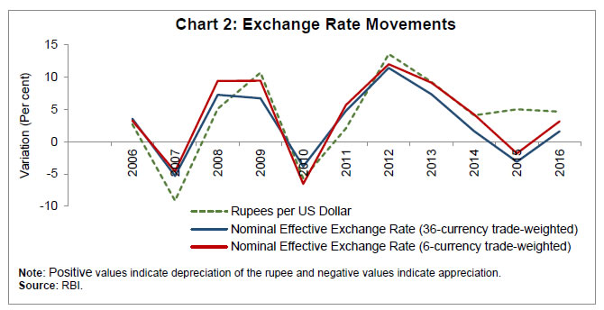 Panel unit root tests suggest that the null of non-stationarity can be generally rejected (or the null of stationarity cannot be rejected in the case of Hadri test) for the panel variables as well as macro variables (Table 1). | Table 1: Unit Root Tests | | (p-values) | | Variable | LLC | HT | BREITUNG | IPS | HADRI | | 1 | 2 | 3 | 4 | 5 | | πcpi-iw | 0.11 | 0.00 | 0.00 | 0.32 | 0.00 | | πcore-iw | 0.00 | 0.00 | 0.00 | 0.07 | 0.01 | | πfood-iw | 0.00 | 0.00 | 0.00 | 0.00 | 0.22 | | ygap | 0.00 | 0.00 | 0.11 | 0.32 | 0.00 | | rain | 0.00 | 0.00 | 0.00 | 0.00 | 0.05 | | Δe | 0.00 | 0.00 | 0.00 | 0.00 | 0.28 | | Δneer36 | 0.00 | 0.00 | 0.00 | 0.00 | 0.99 | | πoil | 0.00 | 0.00 | 0.00 | 0.00 | 0.00 | | πmsp | 0.00 | 0.01 | 0.79 | 0.00 | 0.00 | Note:
LLC: Levin-Lin-Chu; HT: Harris-Tzavalis; IPS: Im-Pesaran-Shin.
The null hypothesis for the LLC, HT, and Breitung tests is: panels contain unit roots versus panels are stationary; for the IPS test, the null hypothesis is: all panels contain unit roots versus some panels are stationary; and, for the Hadri test, the null is: all panels are stationary versus some panels contain unit roots.
Statistics provided in the table are p-values for the relevant null hypothesis. The sample period is 2007-16. Variables with the suffix ‘iw’ indicate the relevant CPI-IW inflation rates.
Source: Authors’ estimates. | Summary statistics of the panel variables indicate that variation over time for each state exceeds variation across states (Table 2). Variation, both within and between, is non-zero, suggesting heterogeneity across states and over time. For the full sample (2007-16), the CPI-IW based core inflation is more volatile than the headline inflation as well as the food inflation, partly reflecting the impact of large variations in house rents due to the award of the sixth Central Pay Commission over the sample period. However, for the shorter period (2011-16), the CPI-C based core inflation is less volatile than the headline, consistent with a priori expectations. The observed heterogeneity suggests the use of panel-based estimation approach. Simple scatter plots of output gap and inflation (both headline and core) show a statistically significant positive relationship between inflation and output gap, suggesting a preliminary evidence in favour of a Phillips curve relationship (Charts 3 and 4; shaded areas in both the charts are the 95 per cent confidence intervals). IV. Estimation Results Static Specifications: CPI-IW We first present results for the static specifications (equations 1 and 2 above) for CPI-IW. The Hausman test favours the random effects (RE) specification over the fixed effects (FE) model and the Breusch-Pagan (BP)-LM test confirms the appropriateness of RE over the ordinary least squares approach, for both core and headline inflation. We report robust standard errors to account for possible heteroscedasticity and residual serial correlation; as a robustness check, we also report PCSE estimates, controlling for heteroscedasticity and first-order residual serial correlation8. | Table 2: Summary Statistics | | Variable | | Mean | SD | Min | Max | | 1 | 2 | 3 | 4 | | Sample Period: 2007-16 | | πcpi-iw | overall | 7.9 | 2.7 | 2.9 | 15.7 | | | between | | 0.6 | 6.9 | 9.2 | | | within | | 2.6 | 2.5 | 14.5 | | πcore-iw | overall | 6.9 | 3.4 | -2.0 | 23.9 | | | between | | 1.0 | 5.6 | 9.4 | | | within | | 3.2 | -0.8 | 21.4 | | πfood-iw | overall | 9.3 | 3.3 | 1.1 | 18.6 | | | between | | 0.7 | 8.0 | 10.9 | | | within | | 3.2 | 1.0 | 17.7 | | ygap | overall | 0.8 | 2.5 | -5.4 | 6.3 | | | between | | 0.5 | -0.1 | 1.6 | | | within | | 2.5 | -4.7 | 6.4 | | rain | overall | -7.6 | 19.3 | -52.6 | 45.7 | | | between | | 8.9 | -22.3 | 7.9 | | | within | | 17.3 | -52.7 | 39.8 | | Δe | overall | 3.9 | 6.6 | -9.1 | 13.5 | | Δneer36 | overall | -2.8 | 5.3 | -11.4 | 5.3 | | πoil | overall | -4.1 | 29.6 | -63.9 | 31.0 | | πmsp | overall | 9.0 | 5.3 | 3.1 | 19.4 | | Sample Period: 2011-2016 | | πcpi-c | overall | 7.2 | 2.6 | -2.5 | 20.9 | | | between | | 0.5 | 6.4 | 8.0 | | | within | | 2.6 | -2.9 | 20.6 | | πcore-c | overall | 6.6 | 1.8 | 3.3 | 10.1 | | | between | | 0.5 | 5.7 | 7.4 | | | within | | 1.7 | 3.2 | 10.1 | | πfood-c | overall | 8.0 | 3.1 | -0.8 | 15.8 | | | between | | 0.6 | 6.8 | 9.0 | | | within | | 3.1 | -0.9 | 15.7 | Note: SD: Standard deviation; Min: Minimum; Max: Maximum.
Source: Authors’ estimates. | 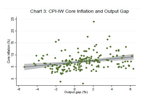 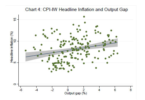 Starting with estimates for the core inflation (equation 1 above) as the dependent variable, all variables have the expected signs and are statistically significant: demand pressures, exchange rate depreciation, and higher oil prices put upward pressure on core inflation (Table 3, panel A)9. Columns 1-3 present results for the RE model10 while columns 4-6 present results for the PCSE model. Furthermore, columns 1 and 4 present the results for the basic Phillips curve specification; columns 2 and 5 present estimates for the augmented specification with the exchange rate proxied by movements in the Indian rupee per US dollar (INR-USD); columns 3 and 6 report results with the 36-currency NEER used to measure the exchange rate dynamics. Even in the basic Phillips curve specification, the coefficient of output gap is on the expected lines (positive) and statistically significant. 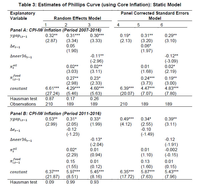 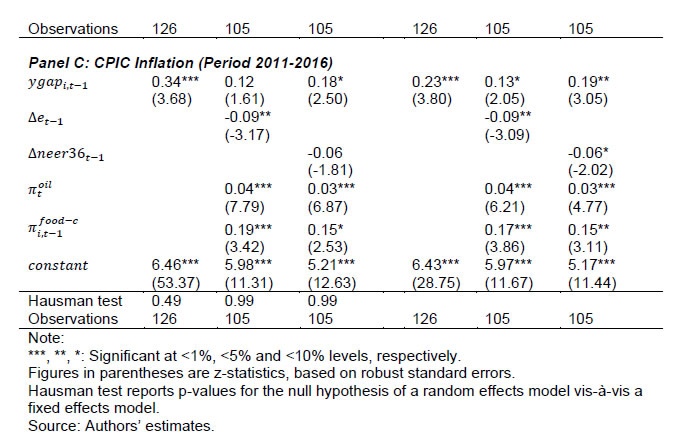 In terms of the preferred PCSE specifications (columns 5 and 6), the point estimates indicate that if the output gap increases by one percentage point, then the core inflation could increase by around 30 basis points. The exchange rate pass-through coefficient is 0.06 when measured by INR-USD and higher at 0.12 when measured by NEER-36; the estimates thus indicate that a 10 per cent depreciation of the domestic currency can lead to an increase of 60-120 bps in core inflation11. The substantial difference is perhaps attributable to the conflicting signals thrown by the alternative exchange rate measures (as discussed earlier and shown in Chart 2) and raises the issue of the appropriate exchange rate measure. The pass-through estimate is, however, comparable to that of advanced economies, and lower than emerging regions provided in IMF (2016) and BIS (2016), perhaps reflective of the lower import content of consumption in the Indian context. Food items have a weight of almost 46 per cent in CPI-IW and high and persistent food inflation can potentially have second-round impact on core inflation and this is borne out by the estimates: an increase of one percentage point in food inflation pushes up core inflation by about 19-24 bps. Turning to the headline inflation, all the variables have the expected signs and are generally statistically significant12. A positive output gap of one per cent can increase headline inflation by around 15 bps (Table 4, Panel A, columns 5 and 6). This is expectedly lower than the core inflation coefficient, suggesting that demand pressures have less impact on food prices. The exchange rate coefficients indicate that a 10 per cent depreciation can increase headline inflation by almost 1.1-1.8 percentage points, with the impact (as in the case of core inflation) being higher for the NEER-36 coefficient vis-à-vis the INR-USD coefficient. Moreover, the exchange rate impact on headline inflation is also higher than that on core inflation, suggesting a stronger exchange rate impact on food prices vis-à-vis non-food items. The MSP policy and crude oil prices have the expected hardening impact on headline inflation, while good rains moderate inflationary pressures. 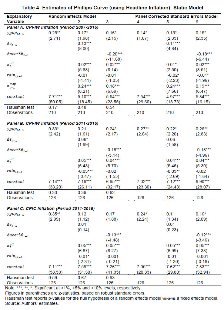 Dynamic Specifications: CPI-IW Moving to the GMM estimates of the dynamic specifications, estimates for both difference GMM and system GMM are presented. The GMM approach can quickly lead to a large number of instruments and an overfitting of the model (Roodman, 2009). Therefore, as a robustness check, we also report results by restricting the number of instruments13. As the results are broadly similar, we focus on the system GMM estimates in the discussion below. Starting with core inflation (Tables 5a and 5b for INR-USD and NEER-36, respectively and the augmented specifications in columns 8-10 of the tables), the coefficient of the first lag of inflation is around 0.5 across specifications, indicative of persistence14. The coefficients of the output gap are at around 0.38-0.49. These coefficients are higher vis-à-vis the static regressions, suggesting an important role of demand conditions in the inflation process: an output gap of one per cent can increase core inflation by close to 40-50 bps. The estimates suggest that the sacrifice ratio – the cumulative output loss that may be needed to reduce inflation by one percentage point – is around 1.5-2.0. The concept and interpretation of the sacrifice ratio is subject to limitations as set out in Kapur and Patra (2000). The exchange rate coefficients are around 0.10 (with the long-run values at 0.12-0.13) when the NEER-36 is employed, close to the static regressions: thus, a 10 per cent depreciation of the domestic currency can lead to an increase of one percentage point in core inflation with a lag of one year and slightly more over the long-run. The exchange rate coefficient, however, loses significance (and is also quite low) when the INR-USD is used. There is evidence of spillover from food inflation, with an increase of one percentage point in food inflation leading to an increase of 15-25 bps in core inflation across alternative specifications. The diagnostic tests are satisfactory: the over-identifying restrictions (Hansen’s J-statistic test15) cannot be rejected at conventional levels; the null of no (second-order) autocorrelation is also not rejected at 5 per cent significance level. 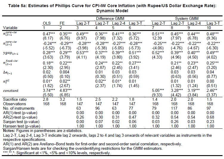 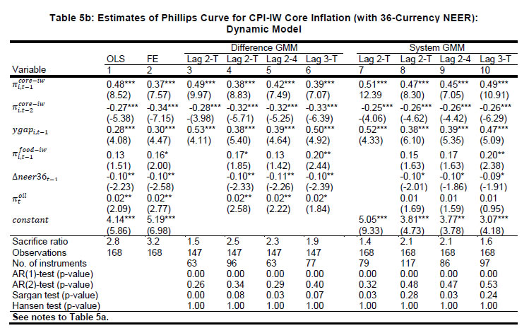 As regards the dynamics of headline inflation, its persistence (0.34-0.48) is slightly lower than core inflation, consistent with a priori expectation (Tables 6a-6b, columns 8-10). As in the case of core inflation, the coefficients on the output gap (0.35-0.49) exceed the corresponding static regression estimates. The exchange rate pass-through coefficient is estimated at 0.08-0.09 (long-run at 0.15-0.16) with INR-USD and (as in the earlier cases) slightly higher at 0.12-0.13 (long-run at 0.20-0.21) with NEER-36. As in the static specifications, the impact of the exchange rate on headline inflation exceeds that on core inflation, perhaps reflective of the relatively greater weight of tradable goods such as food items in headline inflation vis-à-vis core inflation. Amongst other determinants, minimum support prices impart upside pressures on inflation, and good rainfall contains inflationary pressures; higher oil prices contribute to higher inflation, although the estimate is generally not statistically significant16. Consumer Price Index (Combined) Inflation In this sub-section, we turn to the determinants for the CPI-C, which is the nominal anchor of the FIT regime in place since 2014. Given the relatively smaller sample, the results here should be seen as preliminary. In order to assess as to whether the inflation process for the CPI-C is similar to that of the CPI-IW, we also present results for the CPI-IW for exactly the same period (i.e., for 2011-2016). Given the sharp divergence between the INR-USD and the NEER-36 in 2015, in conjunction with the relatively shorter sample size, the estimates with the INR-USD show some puzzling results (with depreciation leading to lower inflation in some specifications). This could be reflecting the fact that inflation moderated in 2015, even as the bilateral exchange rate (vis-à-vis the US dollar) depreciated; in effective terms, the NEER had rather appreciated. We, therefore, restrict our discussion below to the estimates based on the NEER-36. The empirical results for the CPI-C are qualitatively comparable to the CPI-IW, albeit there seem to be some quantitative differences. The estimated impact of demand pressures and the exchange rate on the CPI-C inflation (both core and headline) is less than that for the CPI-IW (for the longer as well as the shorter sample) (Tables 3 and 4, Panels B and C). A lower output gap coefficient for the CPI-C vis-à-vis the CPI-IW indicates a possible flattening of the Phillips curve, with implications for monetary policy: excess demand conditions might have lesser impact on inflation, while any disinflation might need a higher sacrifice of output. The exchange rate (NEER-36) coefficient at 0.06-0.12 for the CPI-C (vis-à-vis 0.12-0.18 for CPI-IW), suggests a relatively lower role for the imported price pressures through the exchange rate channel. 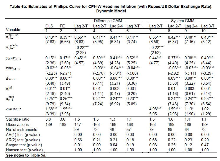 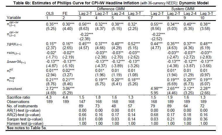 The difference between the results for the CPI-C inflation relative to that of the CI-IW for the common period (2011-16) could be just a reflection of the short sample period and if so, a longer time period might be needed to validate the findings of this paper. The differences in econometric estimates could also be on account of the conceptual and methodological frameworks underlying the CPI-C and CPI-IW. Here, a number of factors are relevant. First, the CPI-IW is restricted to 78 industrially important centres, whereas the CPI-C covers both rural and urban areas. The weight of the rural areas in the CPI-C is more than 50 per cent, whereas this segment was excluded from the CPI-IW. The consumption baskets vary widely across rural and urban areas. For the CPI-C, the food group has substantially less weight in the urban areas relative to the rural areas, while the housing group has no weight in the rural areas (Table 7). The differences in the weighing pattern, along with divergent trends in item-wise inflation rates, can lead to a wedge between the inflation rates across alternative measures of broader inflation, at least over horizons of a few years. For example, within the CPI-C, the rural inflation at 5.5 per cent (average of 2015 and 2016) was higher than the urban inflation (4.2 per cent). | Table 7: Weighing Pattern of CPI-Industrial Workers and CPI-Combined | | (Per cent) | | Group | CPI-IW | CPI-Combined | CPI-Rural | CPI-Urban | | | Base 2001=100 | Base 2012=100 | | Food | 46.2 | 45.9 | 54.2 | 36.3 | | Pan, Supari, Tobacco | 2.3 | 2.4 | 3.3 | 1.4 | | Fuel & Light | 6.4 | 6.8 | 7.9 | 5.6 | | Housing | 15.3 | 10.1 | 0.0 | 21.7 | | Clothing, Bedding & Footwear | 6.6 | 6.5 | 7.4 | 5.6 | | Miscellaneous | 23.3 | 28.3 | 27.3 | 29.5 | | Total | 100.0 | 100.0 | 100.0 | 100.0 | | Memo: | | | | | | Share in CPI-Combined | -- | 100.0 | 53.5 | 46.5 | | Source: Labour Bureau; Central Statistics Office. | Second, the CPI-C is now based on geometric means (for averaging the price relatives of an items across markets/quotations) while the CPI-IW is based on arithmetic means. The geometric means based series is expected to be less affected by extreme values, show lesser volatility and a lower level relative to the arithmetic means based series. The inflation rates for the series using the geometric means during 2014 were less than for the series using the arithmetic means (CSO, 2015), although these can go either way. Third, the index for the housing in the CPI-IW exhibits a step-adjustment [revised twice a year (January and July) and kept constant for the following six months], whereas it is updated every month in the CPI-C. Consequently, the differences in inflation rates across the alternative indicators of inflation can be expected to spillover to the coefficient estimates. A robust assessment of the various hypothesis explored here can be assessed as and when more data become available. Overall, the empirical estimates in this section confirm the presence of a Phillips curve relationship for the CPI inflation (core as well as headline on the one hand and CPI-IW and CPI-C on the other hand), with both demand and supply side factors impinging upon the inflation process. V. Concluding Observations This paper has revisited the issue of determinants of inflation in India in a Phillips curve framework. The paper’s empirical approach makes two key contributions in relation to existing studies in the context of the Reserve Bank moving towards the flexible inflation targeting framework under which the CPI-C is the nominal anchor. First, this paper attempts to model dynamics of the consumer price inflation, whereas the previous studies have mostly been on the determinants of WPI. Specifically, this paper models CPI-IW inflation and a first attempt to model the inflation process for the CPI-C itself. Second, this paper explores the Phillips curve relationship using sub-national data in a panel-approach, whereas all the existing studies have been based on all-India data. Relatively more heterogeneity in inflation rates and output gaps across states vis-à-vis national data can help to decipher better the Phillips curve relationship, apart from providing a robustness to estimates based on national data. This approach is all the more helpful, given the limited time-series data for the new CPI-C series. The estimates in this paper confirm the presence of a conventional Phillips curve specification for consumer price inflation, both core and headline. Excess demand conditions have the expected hardening effect on inflation, with the impact being more on core inflation. Exchange rate movements are also found to have a significant impact on inflation, with appreciation reducing inflation and depreciation leading to higher inflation. Higher minimum support prices results in higher headline inflation, and there is evidence of food inflation spilling over to core inflation. The empirical analysis also suggests some differences between the inflation processes for the CPI-C and the CPI-IW, albeit tentative in view of the limited data availability for the CPI-C series. With this caveat, the results in this paper suggest, first, that the Phillips curve for the CPI-C inflation is perhaps flatter than the CPI-IW inflation. On the one hand, a flatter curve would suggest that excess demand conditions might have a lesser impact on inflation which indicates that any disinflation might need a higher sacrifice of output. Second, the estimates also suggest a somewhat lower role for the exchange rate induced price pressures in the case of the CPI-C inflation vis-à-vis the CPI-IW inflation. Overall, the paper’s findings of demand/supply conditions impacting the CPI inflation suggest a role for a counter-cyclical monetary policy to stabilise inflation and inflation expectations. The paper’s empirical analysis is subject to a few caveats. First, the paper’s sample period covering 2007-16 largely spans a high inflation regime and the pre-flexible inflation targeting regime. With the shift towards the inflation targeting regime in 2014 and the significant disinflation during 2015 and 2016, it would be useful to re-assess the drivers of CPI-C inflation as more data become available. Second, given the limited time series data, the paper has assumed homogeneous slopes across states, and it would be useful to test this assumption contingent on the availability of additional data points. Finally, in view of state-wise GDP data being available on an annual basis, the estimates have been constrained to use annual data for all variables. Quarterly data on output for states would permit a better understanding of the underlying dynamics and the lag structure of the various impacts.
References Aaronson, Daniel and Daniel Sullivan (2000), “Unemployment and wage growth: Recent cross-state evidence”, Economic Perspectives, Vol. 24(2), pp. 54-71, Federal Reserve Bank of Chicago, Abbas, Syed Kanwar (2017), “Global Slack Hypothesis: Evidence from China, India and Pakistan”, Empirical Economics, DOI:10.1007/s00181-016-1207-0 Arellano, M. and O. Bover (1995), “Another Look at the Instrumental Variable Estimation of Error-Components Models”, Journal of Econometrics, Vol. 68, pp. 29-51. Arellano, M. and S. Bond (1991), “Some Tests of Specification for Panel Data: Monte Carlo Evidence and an Application to Employment Equations”, The Review of Economic Studies, Vol. 58, pp. 277-97. Ball, Laurence and S. Mazumder (2015), “A Phillips Curve with Anchored Expectations and Short-Term Unemployment”, Working Paper 39, International Monetary Fund. Blanchard, Olivier (2016), “The United States Economy: Where to from Here? The Phillips Curve: Back to the'60s?”, American Economic Review, 106(5), pp.31-34. Blanchard, Olivier, Lawrence Summers and E. Cerutti (2015), “Inflation and Activity: Two Explorations and their Monetary Policy Implications”, Working Paper 21726, National Bureau of Economic Research. Blundell, R., and S. Bond (1998), “Initial Conditions and Moment Restrictions in Dynamic Panel Data Models”, Journal of Econometrics, Vol. 87, pp. 115-43. Bobeica, Elena and Marek Jarociński (2017), “Missing Disinflation and Missing Inflation: The Puzzles that aren’t”, Working Paper 2000, European Central Bank. Bond, Stephen (2002), “Dynamic Panel Data Models: A Guide to Micro Data Methods and Practice”, Portuguese Economic Journal, Vol. 1, pp.141-162 Central Statistics Office (2015), Consumer Price Index: Changes in the Revised Series (Base Year 2012=100). Chinoy, Sajjid, Pankaj Kumar and Prachi Mishra (2016), “What is Responsible for India’s Sharp Disinflation?”, Working Paper 166, International Monetary Fund. Chowdhury, Kushal and Nityananda Sarkar (2016), “Is the Hybrid New Keynesian Phillips Curve Stable? Evidence from Some Emerging Economies”, Journal of Quantitative Economics, available at: doi:10.1007/s40953-016-0059-y Coen, Robert, Robert Eisner, John Marlin, and Suken Shah (1999), “The NAIRU and Wages in Local Labour Markets”, American Economic Review, Papers and Proceedings, Vol. 89(2), pp.52-57. Coibion, O. and Y.Gorodnichenko, (2015). “Is the Phillips Curve Alive and Well after All? Inflation Expectations and the Missing Disinflation”, American Economic Journal: Macroeconomics, 7(1), pp.197-232. Dua, Pammi and Upasna Gaur (2009), “Determination of Inflation in an Open Economy Phillips Curve Framework: The Case for Developed and Developing Economies”, Working Paper 178, Centre for Development Economics, Delhi School of Economics. Fitzgerald, T.J., B. Holtemeyer, and J.P. Nicolini (2013), “Is there a Stable Phillips Curve after All?”, Economic Policy Paper 13-6, Federal Reserve Bank of Minneapolis. Gordon, Robert (1998), “Foundations of the Goldilocks Economy: Supply Shocks and the Time-varying NAIRU”, Brookings Papers on Economic Activity, Vol. 29, pp.297–333. Government of India (2008), Working Class Family Income and Expenditure Survey, 1999-2000 General Report, Ministry of Labour, Labour Bureau. Goyal, Ashima and Akash Baikar (2014), “Psychology, Cyclicality or Social Programs: Rural Wage and Inflation Dynamics in India”, Working Paper 14, Indira Gandhi Institute of Development Research. Goyal, Ashima and Shruti Tripathi (2015), “Separating Shocks from Cyclicality in Indian Aggregate Supply”, Journal of Asian Economics, Vol. 38, pp. 93-103. Gross, Marco and Willi Semmler (2017), “Mind the Output Gap: The Disconnect of Growth and Inflation during Recessions and Convex Phillips Curves in the Euro Area”, Working Paper 2004, European Central Bank. Kapur, Muneesh and Michael Patra (2000), “The Price of Low Inflation”, Occasional Papers, Reserve Bank of India, Vol. 21(2–3), pp.191–233. Kapur, Muneesh (2013), “Revisiting the Phillips curve for India and Inflation Forecasting”, Journal of Asian Economics, Vol. 25, pp. 17-27. Kiley, Michael (2015), “An Evaluation of the Inflationary Pressure Associated with Short- and Long-term Unemployment”, Economics Letters, Vol. 137, pp.5-9 Kumar, Anil, and Pia Orrenius (2016), “A Closer Look at the Phillips Curve Using State-level Data”, Journal of Macroeconomics, Vol. 47, pp. 84-102 Mazumder, Sandeep (2011), “The Stability of the Phillips Curve in India: Does the Lucas Critique Apply?”, Journal of Asian Economics, Vol. 22, pp. 528-539. Mehrotra, Aaron, Tuomas Peltonen and Alvaro Santos Rivera (2007), “Modelling Inflation in China: A Regional Perspective”, Working Paper 829, European Central Bank Mohaddes, Kamiar and Mehdi Raissi (2014), “Does Inflation Slow Long-Run Growth in India?”, Working Paper 222, International Monetary Fund Osadcha, Margarita (2014), “A State-Level Analysis of the Phillips Curve”, Research Paper 526, Southern Illinois University Carbondale. Patra, Michael and Muneesh Kapur (2012), “A Monetary Policy Model for India”, Macroeconomics and Finance in Emerging Market Economies, Vol. 5(1), March, pp. 16-39. Patra, Michael and Partha Ray (2010), “Inflation Expectations and Monetary Policy in India: An Empirical Exploration”, Working Paper WP/10/84, International Monetary Fund. Patra, Michael, Jeevan Khundrakpam, Asish George (2014), “Post-Global Crisis Inflation Dynamics in India: What has Changed?”, in Shah, Shekhar, Barry Bosworth and Arvind Panagariya (ed), India Policy Forum 2013-14, Vol. 10, Sage Publications, New Delhi, pp. 117-191 Paul, Biru Paksha (2009), “In Search of the Phillips Curve for India”, Journal of Asian Economics, Vol. 20, pp. 479-488. Reserve Bank of India (2002), Report on Currency and Finance 2000-01. ---- (2004), Report on Currency and Finance 2003-04. --- (2014a), Report of the Expert Committee to Revise and Strengthen the Monetary Policy Framework (Chairman: Urjit R. Patel), January. --- (2014b), Monetary Policy Report, September. --- (2016), Monetary Policy Report, October. Roodman, David (2009), “How to do xtabond2: An Introduction to Difference and System GMM in Stata”, The Stata Journal, Vol. 9(1), pp. 86-136 Sen Gupta, Abhijit and Rajeswari Sengupta (2016), “Is India Ready for Inflation Targeting?”, Global Economy Journal, Vol. 16(3), pp.479-509. Singh, B. Karan, A. Kanakaraj and T.O. Sridevi (2011), “Revisiting the Empirical Existence of the Phillips Curve for India”, Journal of Asian Economics, Vol.22, pp.247-258. Smith, Christopher (2014), “The Effect of Labour Slack on Wages: Evidence from State-level Relationships”, FEDS Notes, Board of Governors of the Federal Reserve System. Sonna, Thangzason, Himanshu Joshi, Alice Sebastian and Upasana Sharma (2014), “Analytics of Food Inflation in India”, Working Paper 10, Reserve Bank of India Srinivasan, Naveen, Vidya Mahambare and M.Ramachandra (2006), “Modelling Inflation in India: Critique of the Structuralist Approach”, Journal of Quantitative Economics, New Series, Vol. 4 (2), pp.45–58. Stock J and Watson MW (2009). “Phillips Curve Inflation Forecasts”, In: Fuhrer J, Kodrzycki Y, Little J, Olivei G, Understanding Inflation and the Implications for Monetary Policy, Cambridge: MIT Press, pp. 99-202. Wall, Howard and Gylfi Zoega (2003), “U. S. Regional Business Cycles and the Natural Rate of Unemployment”, Working Paper 2003-030A, Federal Reserve Bank of St. Louis. |