Following the standard stochastic frontier model for cross section analysis (Aigner et al., 1977) later extended to panel data (Battese and Coelli, 1995), let 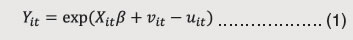
where Yit denotes own tax revenue (OTR)/ taxes on commodities and services (TaxCom), Xit denotes vector of inputs (viz., Log Per capita GSDP, Square of Log Per capita GSDP and Log share of Agriculture in GSDP) affecting tax revenue for the i th state in the t th period and β is a vector of unknown parameters. Error component is decomposed into two parts vit and uit; vit is statistical noise term with symmetric distribution while uit is a non-negative error component representing the time varying technical inefficiency. The inefficiency effects are expressed as an explicit function of state-specific variables and a random error to identify the reasons for differences in predicted efficiencies between states as given below 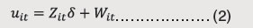
where Wit is a random variable defined by truncation of normal distribution with zero mean and variance σ2 and Zit denotes vector of variables predicting inefficiency (viz., Ratio of transfers in revenue receipts, Aggregate Expenditure to GSDP, Debt-GSDP ratio and VAT Dummy). The estimates of efficiency can be derived once the point estimates of uit are obtained by the following expression; 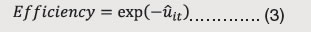
| Table 1: Stochastic Frontier and Technical Inefficiency – Estimates | | | SFA Model 1 | SFA Model 2 | | Log OTR- GSDP | Log TaxCom- GSDP | | Stochastic Frontier | | | | Log Per capita GSDP | 0.299*
(0.032) | 0.281*
(0.021) | | Square of Log Per capita GSDP | -0.0148*
(0.031) | -0.0143*
(0.015) | | Log share of Agriculture in GSDP | -0.0579**
(0.006) | -0.0564**
(0.004) | | Constant | 0.644
(0.365) | 0.67
(0.294) | | Inefficiency Equation | | | | Ratio of transfers in revenue receipts | 0.0222***
(0.000) | 0.0228***
(0.000) | | Aggregate Expenditure to GSDP | -0.0557***
(0.000) | -0.0619***
(0.000) | | Debt-GSDP ratio | 0.00279*
(0.024) | 0.00472***
(0.000) | | VAT Dummy | -0.126***
(0.000) | -0.105**
(0.002) | | Constant | 0.189**
(0.001) | 0.256***
(0.000) | | Usigma Constant | -6.868***
(0.000) | -6.135***
(0.000) | | Vsigma Constant | -4.320***
(0.000) | -4.357***
(0.000) | | Observations | 363 | 401 | | Log-Likelihood | 262.7 | 288.7 | p-values in parentheses
* p < 0.05, ** p < 0.01, *** p < 0.001 |
| Table 2: Sigma Convergence Test | | | SD Model 1 | SD Model 2 | | Year | 0.792*
(0.035) | 1.155***
(0.000) | | Year sq. | -0.000198*
(0.035) | -0.000289***
(0.000) | | Constant | -790.6*
(0.035) | -1153.7***
(0.000) | | Observations | 23 | 25 | | Log-Likelihood | 63.45 | 70.19 | p-values in parentheses
* p < 0.05, ** p < 0.01, *** p < 0.001 | |