Press Release

RBI Working Paper Series No. 02
The Unintended Side Effects of Basel III Liquidity Regulations
on the Operating Target of Monetary Policy
^@Sitikantha Pattanaik
Rajesh Kavediya
Angshuman Hait

Abstract

¹The implementation of Basel III liquidity regulations entails unintended ramifications for the unsecured segment of the money market, and therefore for the operating target of monetary policy. Empirical estimates from a dynamic panel model suggest that under the liquidity coverage ratio (LCR) regime, liquidity constrained banks in India tend to borrow and lend at higher rates in the unsecured segment of the overnight money market. As a result, the weighted average call rate (WACR) – the operating target of monetary policy – is pushed up by about 5 to 7 bps. Estimated results also indicate that borrowing/ lending spreads and volumes in the unsecured money market are sensitive to overall financial soundness of banks.

Key words: Liquidity Coverage Ratio, Basel III, Operating Target of Monetary Policy

JEL Classification: E52, E58, G28

Introduction

The unsecured segment of the money market, or the inter-bank call money market, sets the weighted average call rate (WACR) on a daily basis, which is the operating target of monetary policy in India. By modulating liquidity conditions, the Reserve Bank of India (RBI) aims at anchoring the WACR around the policy repo rate, thereby ensuring effective transmission of monetary policy at the first leg of the term structure of interest rates. The introduction of Basel III liquidity regulations, however, poses potential risks in terms of altering volumes, rates and volatility in the unsecured money market, with corresponding ramifications for the operating framework that guides the implementation of monetary policy (Bonner and Eijffinger, 2013; Schmitz, 2011; Neri, 2012; and Bech and Keister, 2012). Decline in transaction volumes, steepening of the money market yield curve, and the likely sensitivity of borrowing and lending rates to bank specific financial soundness indicators are some of the common potential side effects that have been identified in the literature.

In India, the final guidelines on the Liquidity Coverage Ratio (LCR), Liquidity Risk Monitoring Tools and LCR Disclosure Standards were announced by the RBI on June 9, 2014. As per the phased implementation plan of the LCR norm, banks had to comply with a minimum starting requirement of 60 per cent from January 1, 2015, which was raised to 70 per cent effective from January 1, 2016. Banks have to meet the 100 per cent norm by January 1, 2019. The RBI took adequate precautions to avoid any disruptive impact of the LCR on the money market by allowing reasonable headroom to banks within the prescribed statutory liquidity ratio (SLR). Countries which did not have a statutory arrangement like the SLR to facilitate a non-disruptive adoption of the LCR, had to adopt innovative practices, such as the introduction of a secured committed liquidity facility(CLF) from the central bank – as in Australia and South Africa – to meet the shortfall in high quality liquid assets (HQLA) of banks. Despite these efforts, theoretical and empirical literature generally points to obvious implications of the LCR regime for the unsecured money markets, compelling the need for country-specific assessments of implications from the stand point of identifying and addressing possible challenges for the operating framework of monetary policy. A review of the available limited literature on the subject suggests a wide range of possibilities: the LCR may not constrain the ability of a central bank to implement monetary policy, but it could require tweaking of the operational framework (Bech and Keister, 2012); it may entail certain adverse consequences for money markets (Doran, Kirrane and Masterson, 2014); the effectiveness of monetary policy may be dampened by the LCR norms (Bonner and Eijffinger, 2013); there may not be any obvious detrimental impact on either monetary policy transmission or lending to the real economy (EBA, 2013); and, lack of clarity on the consequences of adoption of LCR norms for the functioning of inter-bank market and monetary policy operations (Noyer, 2012).

This paper, set against this background, outlines major complications that the LCR regime could pose for monetary policy in Section II, based on a review of the relevant literature. Stylised facts covering Indian banks and their money market operations are presented in Section III with a view to drawing inferences on how the LCR regime changed the behaviour of banks, and therefore, the money market trends. Section IV sets out key empirical hypotheses, the methodology for their testing, and an assessment of the plausible implications of the LCR regime for the RBI’s operating framework of monetary policy. Concluding observations are presented in Section V.

II: A Review of Literature

Liquidity transformation, i.e., creating long-term assets based on short-term liquid liabilities has all along been a conventional driving force behind normal banking business. While borrowing short to lend long, banks face a trade-off between minimising their exposure to liquidity risk by holding mostly liquid assets and maximising return by increasing exposure to illiquid assets. Access to funding liquidity (particularly from the money market), market liquidity (that allows use of tradable assets in the portfolio to raise funds when needed), and central bank liquidity (under an operating framework of monetary policy that aims at avoiding deviation of the operating target from the policy interest rate) helps banks in managing this trade-off. Generally, their preference may be to optimise return at the cost of liquidity. By meeting the funding liquidity pressure at the margin through recourse to the money market – both collateralised (secured) and uncollateralised (unsecured) segments – banks tend to sustain the liquidity transformation process. The literature on the relationship between finance and growth – often portrayed as the ';Marx-Schumpeter-Keynes view'; versus the “Mill-Marshall-Solow view'; – also points to the crucial role of funding liquidity at the margin. As per the “credit leads deposit” view, banks could often create long-term assets first if they recognise sound investment projects with higher return opportunities, not constrained by the availability of core deposits, and look for financing subsequently². Before raising more stable long-term financing to fund such asset expansion plans, they may meet the funding requirement from the short-term money market. This liquidity transformation process looked perpetually sustainable before the global crisis. However, when even solvent banks found it difficult to manage the impact of the intense liquidity freeze during the global crisis, the introduction of the new regulatory measures on liquidity to limit the flexibility of banks in managing the trade-off became necessary.

The neglect of liquidity risk was a major limitation of Basel II³, in the context of growing interconnectedness between “funding liquidity”, “market liquidity” and “central bank liquidity”. When markets turn illiquid, and funding liquidity dries up, banks may have to choose between fire sale of assets at lower prices or borrow liquidity at higher cost. However, when well capitalised solvent banks either resort to fire sale or borrow at higher costs, an adverse feedback loop develops, leading to fall in asset prices (that depress the value of collaterals) and hardening of interest rates in money markets (often accompanied by a drop in volumes). In the absence of liquidity buffers, each bank’s action adds to the liquidity pressure, which in turn snowballs into a systemic problem. Neglect of a liquidity buffer at the bank level, thus, does not ensure that a bank internalises the costs of it either selling assets in a bear market or increasing demand for funding liquidity in a tight money market. The self-fulfilling nature of a liquidity freeze, and the scope for “privatisation of profits and socialisation of costs” warranted the introduction of clear regulatory norms on liquidity risks for the banking system. Basel III liquidity regulations intend to do so. First, liquidity norms lower the burden on monetary policy, given the scope for accessing unlimited liquidity from a central bank against eligible collaterals in an endogenous liquidity supply framework. When both funding and market liquidity conditions turn tight, central bank liquidity often becomes the first – rather than the last – resort. Second, it makes banks to internalise the costs of their liquidity risks by making them to hold adequate liquidity buffers, even if that involves some sacrifice of return at the margin. The key question in this context is whether the entrenchment of financial stability through Basel III liquidity regulations comes at the cost of dampening the effectiveness of monetary policy transmission in the money market. According to Bonner and Eijffinger (2013), the positive effects of LCR in terms of reducing the excessive dependence of banks on unsecured inter-bank market may still outweigh “the potential negative implications on monetary policy”.

Bonner and Hilbers (2015) provide a comprehensive review of the historical evolution of the global regulatory approach to manage liquidity risks since 1975, and the rationale justifying the introduction of LCR and the Net Stable Funding Ratio (NSFR) under Basel III liquidity regulations in 2013. While the phased implementation of the LCR has already started – with the minimum of 60 per cent by January 2015, 70 per cent by January 2016 and gradually reaching to full 100 per cent by January 2019, NSFR is expected to be introduced starting in January 2018, and accordingly, the emphasis in empirical research on money market challenges so far largely relates to the LCR. Details of LCR as proposed under Basel III are set out in BIS (2013), and related regulatory guidelines issued in India are available at RBI (2014). In this paper, only specific aspects of the LCR that are relevant to the analysis of money market implications are presented below.

The LCR requirement is that a bank’s stock of high quality liquid assets must exceed its projected total net cash outflows over the next 30 calendar days under stress scenarios (RBI, 2014; BIS, 2013):

(stock of high quality liquid assets)/ (total net cash outflows over the next 30 calendar days under stress scenario) >= 100 per cent (to be achieved in a phased manner by January 2019)

For an assessment of implications for the money market, one needs to particularly look at the impact on secured (collateralised) and unsecured (uncollateralised) money market borrowings/ lending on both the numerator and the denominator of the LCR.

Unsecured wholesale funding in the form of borrowings from the call money market up to 30 days period will have a run off factor of 100 per cent, because they are expected to be repaid or drawn down within 30 days. If a bank creates long term assets using this liquidity which are not eligible to be part of HQLA, then its LCR will fall. In turn, if it holds the borrowed money in the form of cash or uses them to create HQLA, it will be LCR neutral (when LCR is at 100 per cent) or the LCR may increase modestly at the margin (if the LCR position is less than 100 per cent). In other words, the entire borrowed amount will be part of net cash outflows (the denominator of the LCR), and could depress the LCR unless the bank correspondingly increases its HQLA (the numerator of LCR). The incentive to borrow from the unsecured money market, accordingly, will be less, thereby impacting market volumes.

Secured borrowings (against level 1 HQLA), i.e., repo against government securities in the money market or from the RBI will have a runoff factor of zero, and therefore, are LCR neutral. Since excess SLR is a part of level 1 HQLA, converting excess SLR into cash through a repo operation should not have any extra implications for LCR.

The empirical literature broadly points to the following specific aspects that are important to understand the ramifications for monetary policy implementation:

(a) The LCR provides a strong disincentive to lend/ borrow in the unsecured money market, while it favours repos/ reverse repos (Neri, 2012; Bindseil and Lamoot, 2011; BIS, 2015).

(b) Unsecured borrowings of maturity greater than 30 days could be LCR positive, because no repayment would be required within the LCR horizon, i.e., one month. [The aim is to gradually move to a weekly and then daily LCR horizon, so that banks would need to meet the LCR requirement every day (Bonner and Eijffinger, 2013)]. Lower demand at the short-end and higher demand at more than 30-day maturity could steepen the money market yield curve (Smaghi, 2010), and higher volatility of short-end rates could limit the information content of market developments for implementation of monetary policy (Holthausen and Bindseil, 2011). While demand for liquidity may be higher for more than 30-day maturity, there is a disincentive to supply liquidity for this maturity bucket under the LCR, leading to market fragmentation.

(c) Demand for level 1 HQLA assets will increase, impacting yield movements. Correspondingly, demand for non-HQLA assets may decline (Smaghi, 2010). This regulatory distinction between liquid and illiquid assets for the purpose of HQLA eligibility could introduce a cliff effect (Neri, 2012).

(d) The positive externalities of the money market network – or the network effect – will decline (Schmitz, 2011). A vibrant network of banks actively participating in the unsecured money market may often minimise idiosyncratic liquidity shocks from a few participants. The incentive under the LCR to rely less on network and more on own liquidity buffer may increase market volatility.

(e) Behaviour of banks in the money market would constantly change depending on their LCR positions and financial soundness (Bonner and Eijffinger, 2013):

1. Banks operating at very close to the LCR norm pay/ charge higher rates in the unsecured market;

2. During periods of liquidity stress (or tight liquidity conditions) banks operating at close to the LCR norm would reduce lending in the unsecured market;

3. Bank specific factors, such as capital adequacy position, profitability, size, and relationship in the money market network could also influence both lending/ borrowing rates and volumes.

(f) LCR regulations may entail banks adjusting their liquid liabilities more than liquid assets. LCR may not dampen the pro-cyclical behaviour of liquidity in the secured segment of the money market, which in turn may be strongly correlated with leverage (Duijm and Wierts, 2016)

Before the Basel III liquidity regulations came into force, Noyer (2012) was emphatic that “...the new liquidity ratios ...cannot be applied as they stand, as they do not take into account all their consequences and interactions beyond the prudential objectives themselves, which include in particular the functioning of the interbank market, the level of intermediation or the conditions of monetary policy implementation”. Schmitz (2012) was particularly sceptical that “...the international regulatory and central banking community has less expertise concerning the potential negative side effects of international liquidity standards, e.g, on money markets and monetary policy implementation”. Debelle (2015), the Assistant Governor in charge of Financial Markets, Reserve Bank of Australia provides evidence of a marked decrease in wholesale funding of less than 30 days maturity in Australia after the introduction of LCR. The next section sets out stylised facts relating to India, particularly those concerning likely changes in the behaviour of banks in the call money market in the post LCR regime.

III: The Impact of LCR on Money Market – Some Stylised Facts

The banking system in India has all along maintained a higher LCR on an average relative to the prescribed norm of 60 per cent from January 1, 2015 and 70 per cent from January 1, 2016 (Charts 1a & 1b). Since the banking system has all along been above 90 per cent, it may lead one to infer that there should not be any implications of the LCR for the money market in India. In reality, the position of individual banks relative to the prevailing LCR norm is highly divergent; only a limited number of banks operating at very close to the LCR norm may exert pressure on the unsecured segment of the money market.

Before the tightening of the LCR norm on January 1, 2016 to 70 per cent from 60 per cent, about nine banks were below the 70 per cent level in December 2015, and by February 2016, all banks, except one, were above the minimum of 70 per cent (Charts 2a & 2b). Thus, even when a large number of banks may comfortably meet the LCR requirement, only a handful of them falling short of the required HQLA could create compelling conditions for policy changes.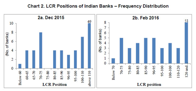

Importantly, despite only a limited number of banks finding it difficult to meet the LCR requirement, the WACR remained under pressure in January 2016 – after the LCR norm was tightened on January 1, 2016 – while in an easing cycle of monetary policy the WACR was expected to remain either close to the repo rate or marginally below the repo rate (Chart 3). On most of the days, the intra-day maximum rate in the inter-bank call market exceeded 25 bps above the repo rate. The RBI provided additional headroom to banks within the prescribed SLR equivalent to 3 per cent of NDTL on February 11, 2016, which helped in addressing the LCR-compliance induced pressure on the WACR. Besides the monetary policy stance, liquidity conditions prevailing at the time of transition to a higher LCR norm is also important to assess the behaviour of WACR, which is appropriately accounted for while estimating the impact in Section IV.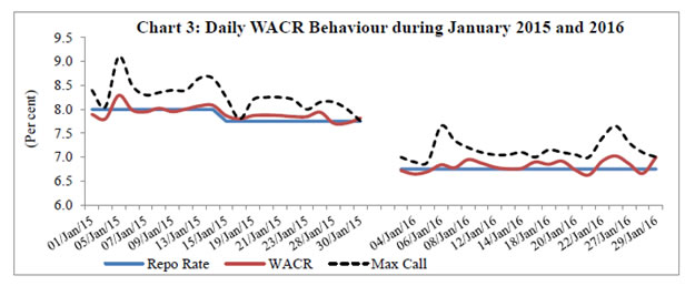

The crucial role of the SLR in ensuring a non-disruptive adoption of the LCR by the banking system in India is evident from Charts 4a & 4b. The SLR is a regulation that requires banks to keep a specific percentage of their net demand and time liabilities (NDTL) in the form of assets primarily comprising cash, gold and Government of India securities. At the time of introduction of the LCR in January 2015, the prescribed SLR was at 22 per cent. Banks also maintain excess SLR for accessing collateralised liquidity from both the RBI and the collateralised segments of the money market. As evident from Chart 4b, while excess SLR – which is eligible to be part of HQLA – falls short of the total HQLA requirement, SLR has all along been higher than HQLA. As a result, if Government securities held within the prescribed SLR is allowed to be reckoned as HQLA, banks would automatically meet the LCR norm comfortably. Recognising this SLR-induced comparative advantage in India for adopting LCR, the RBI allowed up to 7 per cent of NDTL within the SLR to be reckoned towards HQLA (of which 2 per cent of NDTL relates to access to liquidity from the RBI under the MSF facility) on November 28, 2014, i.e., before banks had to comply with the 60 per cent requirement starting from January 1, 2015. Additional headroom equivalent to 3 per cent of NDTL was provided to banks within the prescribed SLR on February 11, 2016 to avoid the liquidity pressure in the money market arising from phased tightening of the LCR norm from 60 per cent to 70 per cent (that became effective from January 1, 2016). On July 21, 2016, additional one per cent of NDTL within SLR was allowed [in anticipation of possible liquidity pressure associated with FCNR(B) redemptions during September to November 2016] thereby raising total carve-out within SLR to 11 per cent of NDTL. As evident from Chart 4a, the carve-out within SLR and excess SLR represent the two predominant parts of total level 1 HQLA of the banking system. Since level 1 HQLA constitutes more than 90 per cent of total HQLA, the carve-out provided within SLR has been critical to the LCR regime in India (Chart 5).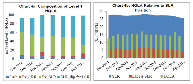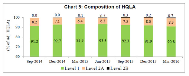

While excess SLR is eligible to be part of HQLA, it also determines the ease at which banks could access collateralised liquidity from the RBI and the money market. The excess SLR holding pattern of banks (in terms of percentage of NDTL) is significantly divergent, and the pattern has not changed much if one compares the period before and after the tightening of LCR norm in January 2016 to 70 per cent (Charts 6a & 6b).

While the operating framework of monetary policy aims at aligning the WACR close to the policy repo rate, borrowing banks often trade liquidity in the unsecured call market at different spreads relative to the repo rate (Charts 7a & 7b). This raises two broad empirical questions: (a) the role of divergent LCR positions of banks in explaining the divergent spreads of WACR of banks relative to the repo rate; and (b) the role of divergent LCR positions of banks in influencing the volume (i.e., borrowing/ lending) in the unsecured money market.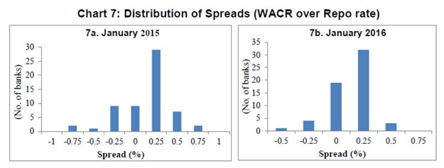

As evident from Chart 8a, banks with LCR in excess of 100 per cent generally borrow less from the call market, though some of them also borrow large amounts. Banks operating at close to the LCR norm borrow different amounts from this market, pointing to no clear relationship between LCR position and call volumes. Importantly, the LCR position of banks and their call market borrowing spreads did not exhibit any distinct pattern (Charts 8b). This is also corroborated by the system level data presented in Chart 9a & 9b, which suggest that call volumes did not fall after either January 2015 or January 2016.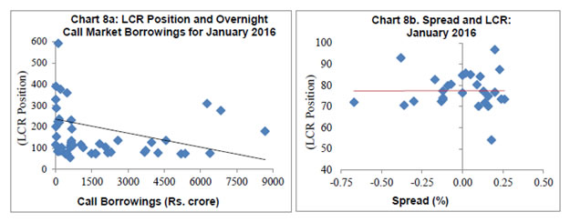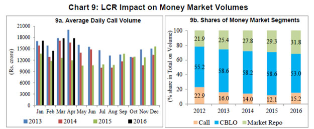

As expected, banks with higher excess SLR also seem to have higher LCR (Chart 10). Given the observed weak relationships at the aggregate level between LCR and spreads/ volumes, it becomes relevant to focus only on such banks which are at close to the LCR norm as against those who may be way above the LCR norm, and then to estimate whether the changed behaviour of the former group of banks in the money market can alter the WACR, even if modestly. This is attempted while empirically estimating the impact in Section IV. Moreover, the microstructure of the money market is important to assess the movements in WACR. Volumes in the overnight segment of the call market in India are highly concentrated in the first and last hour of the day, together accounting for about 70 to 75 per cent of average daily volumes. On an average, call market rate remains high in the first one hour and drops in the last one hour, with the latter conditioned often by co-operative banks supplying their end of the day surpluses at very competitive rates through specific banks in the money market network (Chart 11).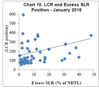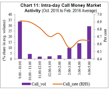

It is important to note that LCR positions and excess SLR holding pattern are highly divergent across different groups within the banking system, i.e., foreign, private and public sector banks (Table 1). The stylised facts presented in this section provide the lead for the assessment of empirical estimates in the next section.

IV: Methodology and Empirical Findings

For empirical analysis, we use monthly panel data for 65 banks covering the period from September 2014 to April 2016. To study the impact of the LCR position of banks on their borrowing/ lending behaviour in the overnight inter-bank call money market, we constructed monthly weighted average borrowing/ lending rates for each of the 65 borrowing/ lending banks using their actual transaction-wise data in the call money market, weighted by corresponding borrowing/ lending volumes. As a regulatory requirement every bank reports, on a monthly basis, their LCR positions as at the end of a month. As the LCR positions widely vary across banks, to study the impact of the LCR on the overnight inter-bank market, a dummy LCRD is constructed which takes the value one if the LCR position of a bank is up to the “prescribed LCR norm” plus 10 per cent, and zero otherwise. Accordingly, banks operating at less than 80 per cent since January 2016 (and less than 70 per cent since January 2015) are considered as LCR constrained for this purpose (i.e., LCRD gets the value of one for such observations). Out of 1300 observations in the panel data set, LCRD takes the value of one for 222 observations.

In order to control for bank specific characteristics, we use bank-wise data on capital to risk weighted asset ratio (CRAR), gross non-performing assets (GNPA) as a ratio of total assets, and return on equity. Also, to control for bank specific structural liquidity pressure in terms of its own credit growth relative to deposit growth, credit to deposit ratio (CD) has been taken as an additional variable. Wherever only quarterly data are available, the quarter-end value is repeated for two subsequent months. Recognising the critical role of the RBI’s liquidity management in influencing the WACR and call market volumes, we introduce average monthly net liquidity adjustment facility (LAF) positions for the system as a whole [as percentage of NDTL of the banking system] as an additional variable in the model, so as to see how the estimated results may change after controlling the impact of liquidity conditions.

Banks with lower LCR positions are expected to borrow at a relatively higher rate in the call market compared with banks that may be comfortably placed in meeting the LCR requirement. Further, it is expected that banks with higher CRAR may get to borrow at lower rates, while banks with higher GNPA may have to pay relatively higher rates. The rate variable WACR is used in terms of a spread over the policy repo rate, on which the impact of the LCR dummy (LCRD), CRAR, and GNPA is examined. To study the volume impact in the call market, bank specific monthly borrowing/ lending volumes are scaled by total assets of the same bank; i.e., total monthly borrowing/ lending volume of a bank as a ratio of its total assets is used to approximate call volume (CallVol). The impact of LCRD and structural liquidity position (CD) on CallVol is examined separately. The “network effect” (NETW), or the preference of a bank to borrow from/ lend to specific banks could at times influence the WACR. This is captured in the model as an additional variable, which is essentially borrowing volumes by a bank from other banks as a percentage of its own total borrowings, weighted by lending of each bank in the system to the concerned bank as a percentage of their respective total lending. (Please see Annex Table 1 for description of all variables used in the model.)

Methodology

A dynamic panel data model is used by employing generalised method of moment (GMM) estimation procedure, to study the impact of the LCR on both WACR and call volumes (separately for lending and borrowings) in the unsecured overnight money market.

A dynamic panel data model of the following type is applied:

By construction, Yi t-1 depends on the individual fixed effects, leading to the endogenity problem. The OLS or fixed effect models generally provide biased estimates for small T and large number of cross section N⁴. Further, inclusion of lagged dependent variables gives rise to the problem of autocorrelation.

To estimate the dynamic panel regression (1), with a larger number of banks in the panel relative to the time period, we use the first difference GMM approach developed by Arellano and Bond (1991).

The first-difference of equation (1) transforms into,

This approach removes the unobserved individual bank specific effects and also addresses the issue of endogenity of explanatory variables by using valid instruments. The first-difference of the panel data helps to remove the time-invariant fixed effects and values (levels) of the lagged dependent variables work as valid instruments for the first-differenced variables, provided that the residuals are free from second-order serial correlation. For testing the absence of autocorrelation, Arellano-Bond test is used, while the validity of the instrument is tested using the Sargan test of over identifying restrictions.

Empirical Findings

Banks that are LCR constrained seem to pay about 7 basis points (bps) higher spread while borrowing in the unsecured money market (Table 2). Also, as expected, banks with higher CRAR tend to pay lower borrowing rates, while those with higher GNPA may face higher borrowing costs. Return on Equity (RoE) and the network effect are not statistically significant in the model.

The LCR constrained banks also tend to lend at a higher rate – by about 5 bps. CRAR and GNPA do not have any statistically significant influence on lending rates. Banks with higher RoE appear to lend at a marginally higher rate than others.

In order to check the robustness of results derived from panel data, a simpler approach is adopted based on regressing the proportion of LCR constrained banks (Prop_LCRD) in the sample of 65 banks (which may vary over time) on the weighted average borrowing rates of these 65 banks at the aggregate level (i.e., weighted by their monthly borrowings from the call money market). The regression results suggest that one per cent increase in the proportion of LCR constrained banks in the panel may lead to an increase in the weighted average borrowing costs by about 2 bps in the short-run and about 10 bps in the long-run (Table 3). However, these results may need to be interpreted with caution as they are based on data for a small sample of 20 observations.

Table 3: OLS estimates of Impact of LCR constrained banks on (Prop_LCRD) on weighted average borrowing cost (WACR_AGG)
	Coefficient	t-Statistic
C	0.94	2.17*
WACR_AGG(-1)	0.82	13.62*
Prop_LCRD	0.018	3.14*
	0.89
LM test F-Statistics	1.58 (0.24)
SE of regression	0.16
No. of Observations	20
Note: t-statistics is based on white heteroskedasticity-consistent standard errors & covariance *: Significant at 5% level.

Coming to the impact of LCR on call market borrowing/ lending volumes, the LCR constrained banks tend to borrow more and lend less (Table 4). The volume impact, though appropriate directionally, is not statistically significant. Banks facing the structural liquidity constraint – in terms of credit to deposit ratio – seem to borrow higher. This is consistent with the “Marx-Schumpeter-Keynes” view presented in Section II. Those with higher GNPA and RoE appear to borrow less in the call market. Other variables are not statistically significant in the estimated model.

In view of the critical role of the RBI’s liquidity management in influencing the WACR, the above estimates could be expected to be sensitive to changing liquidity conditions in the system. To account for liquidity effects, net LAF position (as percentage of NDTL) is introduced as an additional variable in the same model, with borrowing spread as the dependent variable. The relationship between LAF and borrowing spreads is positive and statistically significant. This reflects the endogenous liquidity framework under which the entire liquidity demand is fully offset so as to keep the WACR aligned to the repo rate. As a result, when the LAF deficit is high, money market may exhibit some pressure and borrowing spread remains higher, despite higher liquidity injection by the RBI.

A positive relationship between LAF position and borrowing spread also suggests the possibility of WACR getting aligned to the repo rate better if the system wide LAF deficit is reduced from an average of about one per cent of NDTL to close to neutrality, as announced under the modified liquidity management framework by the RBI in April 2016. Importantly, even after the introduction of the new liquidity variable in the model, LCRD remains a statistically significant determinant of spread. The magnitude of the impact, however, moderates from about 7 bps to 5 bps (Table 5).

While estimating the model, the lag structure for the dependent variable is allowed to be determined within the model automatically, and as a result the number of instruments at 171 appears somewhat high, though still much less than the data points (1300). With a view to checking the sensitivity of the model to lag structure, the model is estimated by restricting the maximum number of lags of the dependent variable to 6, which reduces the number of instruments to 79. While the impact of LAF on borrowing spread increases, the impact of LCR remains nearly unchanged. Robustness checks, thus, validate the sensitivity of the spread to LCR, despite allowing adequate carve out within the SLR to banks to meet the LCR norms.

Taking into account the fact that bank soundness factors are not significant statistically in some of the model specifications, and also the fact that these quarterly numbers are repeated for two months in a difference GMM model in order to make the data frequency consistent with other key variables – particularly LCR, CD ratio and LAF on which data are available on monthly basis – the model is re-estimated excluding these bank soundness variables (Annex Table 2). The overall findings nevertheless do not change – LCR and LAF emerge as the two statistically significant determinants of WACR spread, irrespective of alternative model specifications. Just like the microstructure factors specific to the Indian money market (please see Section III), bank soundness and network effects could influence the WACR, but estimating the impact of such effects quantitatively is not the focus of this paper. While recognising the possible role of multiple factors in shaping the movements of the WACR, this paper provides empirical support for LCR as one such factor, whose estimated impact in the range of 5 to 7 bps does not change much with alternative model specifications.

V. Concluding Observations

The operating target of monetary policy is typically highly sensitive to liquidity conditions and the market microstructure. While proactive liquidity management by the RBI aims at anchoring the operating target to the policy repo rate, its reforms and regulatory measures directed at developing the money market help in addressing frictions arising from the market structure. Since the implementation of the Basel III liquidity regulations, a new source of shock to the operating target, in the nature of unintended side effects of these regulations, has necessitated country specific empirical research to assess the likely magnitude of the impact.

This paper finds that a majority of banks in India are placed comfortably to meet the LCR requirement, without any obvious side effects for the operating target. However, some of the banks which are operating at very close to the prescribed LCR norm, and therefore could be termed as LCR constrained, appear to have altered their activity in the call money market in a manner that has impacted both borrowing/ lending rates and borrowed/ lent volumes. Estimates point to LCR constrained banks borrowing at a higher rate, and under alternative specifications of the model, the WACR is pushed up by 5 to 7 bps. These banks also tend to borrow more and lend less in the call market, and when they lend, they seem to lend at about 5 bps higher spread compared with peers who are better placed in meeting the LCR. Bank soundness indicators also seem to exhibit some influence on the call market rates and volumes. While banks with higher CRAR get to borrow at somewhat cheaper rate, those with higher GNPA tend to pay more. Moreover, banks with higher GNPA and RoE appear to borrow less from the call market. When an additional variable is used in the model to capture the impact of liquidity conditions, the LCR still remains a statistically significant determinant of borrowing spreads. Notwithstanding the friction-less transition to the LCR regime in India on account of the carve-out permitted by the RBI within the existing SLR, the adoption of LCR seems to have posed some side effects on the operating target.

^@Sitikantha Pattanaik is a Director and Rajesh Kavediya is an Assistant Adviser in the Monetary Policy Department and Angshuman Hait is a Director in the Department of Banking Supervision. They are grateful to Professor Subrata Sarkar, Ms. Anupam Prakash, Shri Muneesh Kapur, Dr. Harendra Behera and Shri Joice John for offering useful comments and suggestions on an earlier version of the paper.

¹The views and opinions expressed in this paper are those of the authors and do not necessarily represent the views of the RBI.

²As per the ';Marx-Schumpeter-Keynes view';, investment and innovations are the key divers of growth, and savings could adjust passively, i.e., investment/credit leading savings/deposits in an economy. As per the “Mill-Marshall-Solow view';, however, the causality gets reversed - savings/deposits lead investment/credit and savings is the key growth driver (Solimano and Gutierrez, 2006).

³Capital adequacy related regulations were viewed as sufficient, because when banks are encouraged to hold either less risky assets or adequate capital against risky assets, the former ensures low liquidity risk and the latter, i.e., solvency, ensures access to liquidity from a central bank in the event of liquidity stress. As a result, capital regulations seemed to reduce liquidity buffers in banks before the global crisis (Bonner and Hilbers, 2015).

⁴The bias is due to possible presence of correlation between the regressors and the lagged dependent variable. According to Nickell (1981) the bias tends to zero as T approaches infinity. Even when T is as large as 30, the bias may be 20 per cent of the true value (Judson and Owen, 1999).

References

Arellano, M. and S. Bond (1991), “Some Tests of Specification for Panel Data: Monte CarloEvidence and an Application to Employment Equations,'; Review of Economic Studies, 58,277-297.

BCBS (2013), “Basel III: The Liquidity Coverage Ratio and Liquidity Risk Monitoring Tools”, Basel Committee on Banking Supervision, BIS, January.

Bech, M. and T. Keister (2012), “On Liquidity Coverage Ratio and Monetary Policy Implementation”, BIS Quarterly Review, December.

Bech, M. and T. Keister (2013), “Liquidity Regulation and the Implementation of Monetary Policy”, BIS Working Paper No. 432, October.

Biais, B., F. Declerck, and S. Moinas (2016), “Who Supplies Liquidity, How and When?”,BIS Working Paper No. 563, May.

Bindseil, U. and J. Lamoot (2011), “The Basel III framework for liquidity standards and monetary policy implementation”, Humboldt-Universität zu Berlin SFB 649 Discussion Paper 2011-041, available at http://edoc.hu-berlin.de/series/sfb-649-papers/2011-41/PDF/41.pdf.

Bonner, C. and S. Eijffinger (2012a), “Basel Liquidity Rules and their Impact on the Interbank Money Market”, VOX, CEPR’s Policy Portal, October available at http://voxeu.org/article/impact-basel-liquidity-rules-interbank-money-markets.

Bonner, C. and S. Eijffinger (2012b), “The Impact of the LCR on the Interbank Money Market”, DNB Working Paper No. 364, DeNederlandscheBank, December.

Bonner, C. and P. Hilbers (2015), “Global Liquidity Regulation – Why Did It Take So Long”, DNB Working Paper No. 455, DeNederlandscheBank, January.

Bouwman, C. (2013), “Liquidity: How Banks Create It and How It Should Be Regulated?”, In A.N. Berger, P. Molyneux and J.O.S. Wilson (eds.),The Oxford Handbook of Banking, 2nd Edition, Forthcoming.

CGFS (2015), “Regulatory Change and Monetary Policy”, Committee on the Global Financial System and the Markets Committee, CGFS Papers No. 54, BIS, May.

Crandall, L. (2016), “How should Central Banks Steer Money Market Interest Rates?”, Prepared for the workshop – Implementing Monetary Policy Post Crisis: What we have learned? What we need to know?, Columbia SIPA and the Federal Reserve Bank of New York, May 4 available at https://www.newyorkfed.org/medialibrary/media/newsevents/events/markets/2016/frbny-columbiasipa-loucrandall-presentation.pdf.

Debelle, G. (2015), “Some Effects of New Liquidity Regime”, Speech at 28th Australasian Finance and Banking Conference, Sydney, December 16 available at http://www.rba.gov.au/speeches/2015/sp-ag-2015-12-16.html.

Dodd, R. (2012), “What are Money Markets?”, Finance & Development, IMF, June 2012, Vol. 49, No.2 available at http://www.imf.org/external/pubs/ft/fandd/2012/06/pdf/basics.pdf.

Doran, D., C. Kirrane and M. Masterson (2014), “Some Implications of New Regulatory Measures for Euro Area Money Markets”, Central Bank of Ireland, Quarterly Bulletin, January, pp. 91-102.

Duijm, P. and P. Wierts (2016), “The Effects of Liquidity Regulation on Bank Assets and Liabilities”, International Journal of Central Banking, Vol. 12, No. 2, June, pp. 385-411.

EBA (2013), “Report on appropriate uniform definitions of extremely high quality liquid assets (extremely HQLA) and high quality liquid assets (HQLA) and on operational requirements for liquid assets under Article 509(3) and (5) CRR”, European Banking Authority, December 20.

Judson, R. and A. Owen (1999), “Estimating Dynamic Panel Data Models: A Guide for Macroeconomics”, Economic Letters, 65, pp. 9-15.

Liebmann, E. and J. Peek (2015), “Global Standards for Liquidity Regulation”, Current Policy Perspectives No. 15-3, Federal Reserve Bank of Boston, July.

Lnaba, K., R. O’Farrell, L. Rawdanowicz, and A. Christensen (2015), “The Conduct of Monetary Policy in the Future: Instrument Use”, Economics Department Working Papers No. 1187, ECO/WKP(2015)5, Unclassified, OECD, March.

Neri, M. (2012), “The Unintended Consequences of the Basel III Liquidity Risk Regulation”, June available at http://ssrn.com/abstract=2096821 DOI: 10.2139.

Nickell, S. (1981), “Biases in Dynamic Models with Fixed Effects”, Econometrica, 49 (6), 1417-1426.

Noyer, C. (2012), “Basel III – CRD4: Impact and Stakes”, Speech at the Autorite de controle prudential (ACP) conference, Paris, 27 June 2012 available at http://www.bis.org/review/r120703b.pdf.

RBI (2014), Basel III Framework on Liquidity Standards – Liquidity Coverage Ratio (LCR), Liquidity Risk Monitoring Tools and LCR Disclosure Standards, RBI/2014-15/328, DBR.BP.BC.No.52/21.04.098/2014-15, dated November 28, 2014 available at https://rbidocs.rbi.org.in/rdocs/notification/PDFs/ACLCR28112014.pdf.

Ruth A. Judson and Ann L. Owen (1996), “Estimating Dynamic Panel Data Models: A Practical Guide for Macroeconomists”, Federal Reserve Board of Governor, January.

Schmitz, S. (2012), “The Impact of the Basel III Liquidity Standards on the Implementation of Monetary Policy”, September available at http://ssrn.com/abstract=1869810.

Solimano, A. and M. Gutierrez (2006), “Saving Investment and Growth in the Global Age: Analytical and Policy Issues”, In A. Dutt and J. Ross (eds.), Handbook of International Development, Vol. I, Chapter 6, Edward Elgar Publishers, UK and US.

Vishwanathan, N.S. (2015), “Basel III Liquidity Risk Framework – Implementation and Way Forward”, Speech delivered at Hyderabad on November 27.

Annex Table 1

Description of Variables

Annex Table 2