Press Release RBI Working Paper Series No. 05
India’s Potential Output Revisited
@Barendra Kumar Bhoi and Harendra Kumar Behera Abstract *Estimates of potential output have been revised downward across countries in the post-crisis period. In India, the debate on potential GDP and output gap has been intensified due to revision in the GDP estimates with change in base year and its underlying methodology consistent with international best practices. In view of these, an attempt has been made for the first time in India to estimate potential GDP and output gap on a quarterly basis by using production function approach in addition to revisiting the estimates of potential output by conventional statistical methods for the period 1980Q2 – 2015Q4. The findings suggest that India’s potential growth, which had accelerated to around 8 per cent during 2003-2008, decelerated considerably in the aftermath of the global financial crisis to about 7 per cent during 2009-2015, mainly due to decline in contribution of total factor productivity and deceleration in the growth of capital stocks. The estimates further suggest that output gap, i.e. the percentage deviation of actual output from its potential level, has been negative since Q3 of 2012, though the gap is closing slowly. Key to accelerate growth as well as potential output in India lies with higher level of capital formation as its contribution dominates vis-à-vis the contribution of labour and total factor productivity. Key words: Potential output, Business cycle, Production function, Kalman filter. JEL Classification: E32, E23, E52, E3, C32 I. Introduction The estimates of potential output and output gap are critical inputs in many areas of economic policy making. Being an indicator of standard of living, potential growth is important for structural reforms while output gap – a key indicator of inflation pressures in the economy – is crucial for monetary policy making. Unfortunately, however, these are not observable and therefore, require to be estimated. Indeed, important policy mistakes have been made as these estimates turned out to be wrong (Cotis et al. 2004). In the post-crisis period, many countries experienced a sharp downward revision in the medium-term growth prospects. There is a concern that sluggish growth in advanced economies (AEs) in recent years is structural and, therefore, tepid growth would continue over the medium term, spilling over to emerging market economies (EMEs) through different channels. The April 2015 issue of World Economic Outlook of the International Monetary Fund (IMF) finds that potential growth across countries has declined in recent years, with AEs experiencing the decline much before the EMEs, driven mainly by lower total factor productivity growth and deceleration in growth of working age population. According to IMF estimates, potential growth in AEs has declined from 2.4 per cent to 1.9 per cent during 2001-2007 and further to 1.5 per cent during 2013-14, whereas, it increased from 6.1 per cent to 7.4 per cent in EMEs during the pre-crisis period and declined to about 5.5 per cent during 2013-14. The most recent studies in the Indian context provide a wide range of estimates of potential growth (6 - 8 per cent). These studies used old series of gross domestic product (GDP) and found that the potential growth has declined significantly during post-crisis period (Blagrave et al. 2015; Anand et al. 2014; RBI, 2014; Mishra, 2013). India has recently revised its estimates of GDP to improve coverage, incorporate new methodology and align it with global best practices in addition to revising the base year. The recent revisions in national accounts data pose a challenge in terms of assessing the state of the business cycle and the position at which the economy is poised on it. In February 2015, the Reserve Bank of India and the Government of India have agreed to an institutional architecture that empowers RBI to pursue price stability as the primary objective of monetary policy. To achieve price stability, it has become all the more important to understand whether there is any excess demand or excess supply in the economy. In this context, a correct assessment of output gap is crucial to monitor the inflationary pressures in the economy. In India, the real GDP growth has decelerated significantly from around 9.5 per cent during 2005-2007 to about 5 per cent in 2012-13. The correct measurement of potential output will be helpful to understand whether the recent slowdown is due to change in trend or due to cyclical factors. Though growth has recovered in subsequent years, persistent decline in capital goods production and deceleration in capital goods imports might have impacted India’s potential growth adversely. The derived incremental capital output ratio (ICOR), on an average, was higher in the post-crisis period implying possible decline in potential growth in India. In view of the above, it is vital to revisit the estimates of potential output, particularly, the output gap, by using the new GDP data. This study tries to estimate potential output of India employing various statistical filters along with structural economic model. The rest of the paper is organised as follows. Section II presents methodological issues followed by a brief review of the literature in Section III. The empirical results of the study are analysed in Section IV and Section V provides concluding observations. II. Alternative Methods for Estimating Potential Output Potential output generally refers to the level of output that is consistent with full capacity utilisation along with low and stable inflation. In purely statistical sense, however, trend level of observed output is also considered as potential output. According to the Congressional Budget Office (CBO, 2004), the trend level of output is purely a statistical concept which cannot be interpreted as maximum sustainable output, as pertinent economic variables such as capacity utilisation and inflation are not taken into account. When the actual output exceeds the potential output, i.e. the output gap becomes positive, the aggregate demand increases leading to inflationary pressures, assuming supply side factors to remain constant in the short-run. This happens mainly because of rapid economic growth that puts upward pressure on wages and other production costs in a competitive environment. The output gap is typically estimated at levels rather than growth rates. An economy grows much faster as compared to its potential during the time of recovery from its trough, which is not inflationary if the output gap in terms of level is still negative. The measurement of potential output is normally connected with business cycle decomposition by separating trend or permanent component of a series from its transitory or cyclical component. Various methods for estimating potential output and output gap are available in the literature. The methods to estimate potential output can be broadly categorised into three groups: (i) purely statistical methods (e.g. time trend estimation, statistical filters, etc.), (ii) methods that combines structural relationships with statistical methods (e.g., Kalman filter) and (iii) structural methods which are based on economic theory (e.g., production function approach). While the filtering method dissects a time series into permanent and cyclical components purely in a mechanical way, the production function approach attempts to isolate the effects of structural and cyclical influences on output using economic theory. The semi-structural methods like Kalman filter uses economic relationships along with statistical method to derive the potential output from the observed output. While production function approach is treated to be superior as it provides economic explanation for the movement of potential output and helpful for simulation exercises, the univariate statistical filters like Hodrick-Prescott (HP), Rotemberg and Band-Pass (BP) are subject to endpoint problems due to the one-sidedness at both ends of the time series. Despite having their own merits and demerits, we have chosen both the production function approach and statistical methods (the deterministic trend, Hodrick-Prescott filter, Band pass filter and Beveridge-Nelson decomposition) and compared their results with potential output derived through Kalman filter, which combines both statistical methods and structural approach. Deterministic Trend Potential output can be estimated by using the following trend methods: yt = α + βt + εt (1)
yt = α + βt + γt2 + εt (2) where yt is log of real GDP, ‘t’ is time trend and εt is residual. The estimated yt from any of the above regression is the potential output in log terms. The main limitation of linear trend method is that the assumption of constant rate of growth of potential output does not hold well over the sample. Further, the estimated output gaps based on the above methods are sensitive to sample period. For example, if the sample starts at the lowest point of the recession, the slope of the trend line fitting the series becomes steeper, making the gap between actual and potential output at the end of the sample smaller (de Brouwer, 1998). Since the trend is deterministic and the stochastic trend is not fully eliminated, the estimated potential output and output gap (εt) can be biased. Hodrick-Prescott (HP) Filter 
where λ is a weighting parameter that determines the degree of smoothness of the trend relative to output gap. A low value of λ produces the trend output much closer to actual output, whereas a high value of λ produces the trend output that converges to linear trend. Therefore, λ also determines how fast actual output is brought in line with the potential output and how long is the business cycle on average. Following the standard practice for quarterly data, we have used λ=16001. The main problem with HP filter is that the trend follows closely the actual value of the output towards the end of the sample period in the absence of predicted output levels and, therefore, fails to produce unbiased results. To tackle this problem, it is often suggested to consider forecasted output levels for extended sample period. Eight quarter ahead ARIMA based forecast has been used in this paper to take care of endpoint problem. Another limitation of the HP filter is about its treatment of structural breaks that tend to be smoothened by the filter. It is also not possible to create confidence bands to determine the uncertainty of the estimation in case of this filter. Nevertheless, this method is very popular because of its simplistic nature that captures non-linear trend in the potential output. Moreover, the output gaps derived from this filter turn out to be stationary over a wide range of smoothing values. Band Pass (BP) Filters While HP filter eliminates low frequency cycles from data to produce trend series, the BP filter estimates the cycle taking a two-sided weighted moving average of the data where the frequency of cycles pass through a band. The main focus of this filter is to eliminate very slow moving (trend) components and very high frequency (irregular) constituents, while retaining intermediate (business cycle) components. Basically, the underlying time series is a weighted sum of changing cyclical frequencies in this type of method. Thus, the BP filter as developed by Baxter and King (1995) can be stated as:  where cycle is a 3 year weighted average of actual output (yt) and αi corresponds to the weights of frequency response function derived from the inverse fourier transformation. The main problem of the Baxter and King (BK) filter is that output gap or cycle cannot be estimated for the initial and last 3 years of the sample. Therefore, the BP filter, as proposed by Christiano-Fitzgerald (2003), is used to estimate the output gap and potential output for the full sample period. The weights for lags and leads are of same length and time-invariant in case of BK filter (i.e. a fixed length symmetric filter), while the weights on the leads and lags are allowed to differ and is time-varying in Christiano-Fitzgerald (CF) filter (i.e. an asymmetric filter).While applying the CF filter, the critical frequency band to be assigned to the cycle has to be exogenously determined. In this study, the band for cycle is chosen as 6 to 32 quarters in line with the standard practice. Though the BP filters produce much smooth estimates for cycles, the non-cycle portion include irregular components and, therefore, should not be strictly treated as trend. Beveridge-Nelson Decomposition Beveridge and Nelson (1981) method of trend-cycle decomposition of a time-series is based on following assumptions: (a) the observed series is an ARIMA process and, therefore, the growth of that series is stationary; (b the long-run forecast of the series is same as the trend; (c) both the permanent and cyclical components are impacted by a common (unidentified) shock; and (d) the ARIMA specification chosen for trend-cycle decomposition is correct. Since this is a backward looking filter, it has no end-point problem. However, it generates very noisy cycles and are sensitive to model specification. Further, estimated cycles are sometimes negatively correlated with growth of the observed series. Unobserved Component Models The unobserved component model separates the unobserved variables such as potential output, potential growth and output gap from the observed GDP series for a given structural/statistical relationship among these variables. Once the relationship is specified in the state space form and the initial values for the unobserved state vector are provided, the unobserved variables can be estimated by Kalman filter2. Kalman filter uses the initial values for the unobserved state vector to predict the unobserved variables and then updates the guesses based on the prediction errors. When all observations have been processed, the smoothing equations give the best estimators of the unobserved variables based on all the information. Kalman filter can be of univariate type considering only one variable or multivariate type while considering more than one variable. The univariate Kalman filter method is considered to be the simplest way of estimating potential output, which uses only real output data. Univariate Kalman Filter 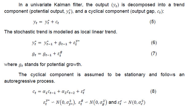
Multivariate Kalman Filter As against the above mentioned univariate filter which considers only GDP to extract potential output, multivariate framework takes into account other economic variables and estimate the potential output using a meaningful economic relationships among these variables. To apply the multivariate Kalman filter, one has to first construct a system of behavioural equations (also called observation equations) consisting, for example, IS curve, Phillips curve, Okun’s law and/or a wage equation. Then assumptions have to be made about the stochastic properties of potential output, which need to be represented in the form of state equations. In this study, the model includes an equation for Phillips curve in addition to eqs. (5) – (8) as given below: 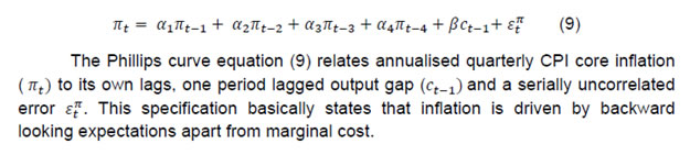
The above equations (5) to (9) can be conveniently translated into a state-space model and estimated using maximum likelihood to derive unobservable variables like potential output, potential growth and output gap. Production Function An alternative to the above statistical methods, the potential output could be estimated using structural approach on the basis of a production function. Let us consider a Cobb-Douglas production function: yt = αlt + (1 - α)kt + tfpt (10) where all the variables are in logarithms, yt is output, lt is effective labour employed, kt is capital stock at time t and tfpt is total factor productivity. While α measures the labour share, (1 - α) measures the capital share. The above Cobb-Douglas production function assumes constant returns to scale. The estimation of potential output involves a few steps: (i) estimation/ determination of labour share based on historical data; (ii) estimation of total factor productivity as Solow residual (i.e. output less the weighted sum of labour and capital inputs); (iii) derivation of trend of total factor productivity and potential labour and capital; and (iv) potential output is estimated based on the values of coefficient and variables obtained in the previous step. However, production function approach is subject to criticisms as it is based on a few assumptions about the functional form, potential labour and capital. The method also uses simple detrending procedures like the HP filter to obtain potential labour or trend productivity, which has a significant bearing on the gap estimate. Once potential output is estimated, the potential growth and output gap can be derived by taking percentage change of the potential output and taking percentage deviation of actual output from its potential level, respectively. Thus, the potential growth and output gap are worked out as: 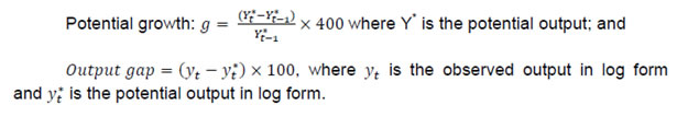
III. Literature Though potential output is very important for policy making, there seems to be no consensus amongst economists regarding the best method to estimate it. Different countries and organisations use different methods and no method has been able to provide consistently robust estimates. The debate is intense in both estimation and treatment of potential output. Keeping the debate aside, we have reviewed here the findings of various studies in Indian context. Generally, different statistical filters like the HP filter and BP filter are being used to estimate the potential output in Indian context (Donde and Saggar, 1999; Ranjan et al. 2007; Bordoloi et al. 2009; Mishra, 2013). Using monthly Index of Industrial Production (IIP) data and a set of statistical filters along with structural VAR method, Bordoloi et al. (2009) found that India’s a potential growth ranges from 8.2 to 10.2 per cent. Employing the same methods on quarterly GDP data, they found that India’s potential growth varies in the range of 8.1 - 9.5 per cent. The estimates seem to be on higher sides as these are biased towards the high growth rate observed during the period when the study was conducted. Similarly, Goyal and Arora (2012) employing SVAR approach and using WPI inflation and IIP growth, found a 9 per cent potential growth for the Indian economy. Using a set of both univariate and multivariate filtering techniques as well as production function approach, Mishra (2013) estimated India’s potential output growth to be in the range of 7.7 – 8.2 per cent for 2011. She found that potential growth increased sharply during 2002 -2007 to about 7.6 per cent from 5.6 per cent during 1997 – 2001. She also found a positive output gap of 0.7 per cent for 2011, which had declined by 0.2 percentage points from its 2010 level. Employing similar methodology like Mishra (2013), Anand et al. (2014) estimated a decline in India’s potential growth from about 8 per cent in pre-global financial crisis period to about 6-7 per cent in recent years. The analysis from their growth accounting exercise suggests that the growth slowdown was mainly driven by decline in trend TFP growth. They further noted that heightened regulatory and policy uncertainties, delayed project approvals and implementation, continued bottlenecks in the energy sector as well as reform setbacks were the main contributing factors for investment slowdown and sluggish TFP growth. Blagrave et al. (2015) provide estimates of potential growth and output gaps for 16 countries using the multivariate filter developed by Benes et al. (2010). Their estimates indicate that India’s potential growth has declined from its peak of above 8 per cent in 2007 to below 6 per cent by 2012 and output gap has turned negative since 2012. Ranjan et al. (2007) is the only study which has estimated the production function for India using data for 1980 to 2004 to provide potential output growth. They found that the potential output growth was 6.6 per cent. Oura (2007) who has estimated the potential growth at 8.0 per cent for the medium-term but pointed out that the medium-term potential growth estimates have risks on both sides, as productivity gains and investment could be volatile, but reforms could sustain the productivity growth. This particular estimate could be viewed as an overestimation because the trend around that time coincided with the high growth phase and the resulting assumptions about the inputs and total factor productivity (TFP) growth appear to be optimistic. Assuming relatively higher TFP growth at 2.5 per cent and capital share of 0.35, Rodrik and Subramanian (2004) projected a potential growth of over 7.0 per cent for India. Similarly, another study by Poddar and Yi (2007), taking TFP growth at 3.3 per cent, found that India’s potential growth could be about 8 per cent until 2020. Their estimate seemed to be biased upward as it was based on high productivity growth and assumed high human capital growth which was quite different from other studies. Long-term output growth estimates relating to different time periods in the past based on the production function approach suggests a range of 6.5 – 8.0 per cent (Table 1). If one applies the assumptions/estimates of elasticities from their studies to the updated data series, the potential growth would be in the range of 5.5 – 7.6 per cent. | Table 1: Estimates of Potential GDP growth for India | | | Bosworth & Collin (2007) | Rodrik & Subramanian (2004)$ | Ranjan et al. (2007) | Poddar
& Yi (2007) | Mishra (2012) | Our Estimate# | | Study/Assn. period | 1993-2004 | - | 1980-2004 | 2003-2005 | 1982-2011× | 1980-2014 | | TFP growth | 2.3 | 2.5 | 1.3* | 3.3 | 3.6 | 1.7 | | Capital Share | 0.40 | 0.35 | 0.76 | 0.33 | 0.30 | 0.69 | | Labour Share | 0.60 | 0.65 | 0.24 | 0.67 | 0.70 | 0.31 | | Human capital growth | 0.67 | | | 2.2 | | | | | | | | | | | | Estimated PO growth in the study | 6.5 | 7.0 | 6.6 | 8.0 | 7.5 | | | Estimating PO growth (1992-2014) based on updated data taking the assumptions given in studies. | 6.0 | 5.5 | 7.0 | 7.6 | 5.7 | 6.6 | $: The estimated potential growth for 1980-1999 was 5.7 per cent and they have provided the projection of potential growth of 7 per cent through 2025.
#: Based on annual data on new GDP, net capital stocks and organised sector employment.
×: Assessment period is for 2008-2011 for calculating potential growth as against the study period (1982-2011).
*: TFP growth is worked out based on their estimates on elasticities and using GDP growth, labour and capital stocks data. | IV. Empirical Estimation The main objectives of the paper are to estimate potential growth and output gap for India. According to de Brouwer (1998), there is no method that provides the estimate with certainty; rather, all estimates form an information set. Therefore, our objective in this paper is to obtain an information set that allows us to refine a ‘representative’ output gap which can be used with confidence for monetary policy making in India. To do so, potential output is estimated using a battery of statistical and structural methods and the estimates are combined using principal component analysis to produce a composite output gap estimate. Data Potential output estimation requires long time series data, which is a major constraint in the Indian context. In addition to that, large scale data revision adds complexity to the estimation of potential output. Statistical methods use past data as the only input, and unless structural factors driving data revisions are known and explicitly modelled, the path of potential output would invariably follow the actual data. Given the limitations of filtering methods, in particular loss of accuracy towards the end of the sample, sensitivity to choice of the appropriate length of smoothing parameter, lack of economic content in the filter approach, potential output estimates based on a production function approach provides a useful cross check. In the absence of a high frequency and updated data on capital stock and labour, it becomes difficult to generate an estimate that could be useful for real time policy making. However, an attempt is made in this paper to construct long time series quarterly data and provide output gap and potential growth estimates based on production function approach as a useful alternative compared to the same estimated by other methods. To estimate potential output, quarterly data for the period 1980Q2 (i.e. April-June of 1980) through 2015Q4 have been used. This paper uses gross value added (GVA) data to estimate India’s potential output. New GDP data (i.e. GVA, base year 2011-12) are available from 2011Q2 to 2015Q4 and GDP at factor cost data (base year 2004-05) are available for 1996Q2 – 2012Q3. Therefore, GVA data prior to 2011Q2 are estimated through splicing method3. Annual spliced GVA is converted into quarterly frequency for the period 1980Q2 to 1996Q1 employing Chow-Lin method and using quarterly index of industrial production as an indicator. Annual data on net capital stock is available since 1980 through 2011 for 2004-05 base and 2011 to 2014 for 2011-12 base. These two series are combined using splicing method and the series is extended from 2013-14 to 2014-15 using growth rate of the previous year. Annual change in capital stock is converted into quarterly series through Chow-Lin method by using quarterly real gross capital formation as an indicator. The quarterly change in net capital stock then transformed into quarterly net capital stock by simply adding them with the initial level of capital stock. In India, data on CPI-combined (sub-group wise) are available since January 2010 and CPI for Industrial Workers (sub-group wise) are available for longer period; the CPI-combined is estimated backward by establishing a relationship between these two series for the common sample period. The core CPI inflation is calculated considering the exclusion based CPI, i.e. overall CPI less food and fuel. Both quarterly GDP and CPI series are adjusted for seasonality using X-13 ARIMA-SEATS. The official employment data on quarterly frequency for India is not available and therefore, collected from Thomson Reuters Datastream. Results In this paper, we estimate the growth rate of potential output and the output gap using three different methods: (i) a production function approach, (ii) a Kalman filter approach (multivariate), and (iii) purely statistical methods (HP, BK, CF and BN). Also, quadratic trend method and one-sided HP filter4 are employed to assess potential growth and output gap. The simplest way to produce potential/trend level of output is the trend method, which estimates potential output solely from information contained in the actual output series. Figure 1 presents both actual output along with the potential output based on a quadratic trend. As per this approach, the potential growth for 2015Q4 is 8.3 per cent. Due to the revision in the GDP data and resulting large level changes in the last four years, a simple trend approach may be misleading. 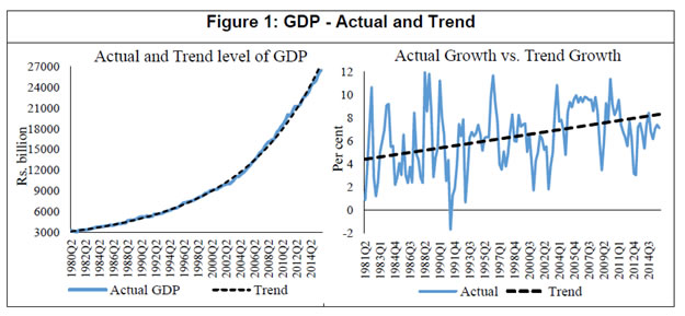 As mentioned before, filter based methods mislay their accuracy towards the end of sample. To address the problem of end-point uncertainty, an ARIMA (3, 4) model is used to generate out of sample forecast of GDP series up to 2019Q1 and this extended sample period is used in case of the techniques sensitive to end-of-sample problem, viz. two sided HP and BP (both CF and BK) filters. A multivariate Kalman filter is also employed to derive potential output, potential growth and output gap. The output gap (i.e., actual output minus potential output) estimates based on pure statistical filters, Kalman filter and quadratic trend are presented in Figure 2. As shown in this figure, the output gaps are highly correlated and broadly consistent across history. While the estimated cycles observe identical peaks and troughs it is notable that the one-sided HP- and trend – based output gaps have higher amplitudes. It is also important to note that estimates move very closely until early 2000s and the divergence has increased thereafter. However, all the estimates suggest that the output gap has been negative since Q3 of 2012, reflecting the domestic policy drift and global uncertainty resulting in a slowdown of the Indian economy. 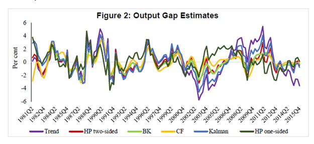 Output gap estimates based on univariate BN method5 is provided separately in Figure 3, as it is a different class of model altogether, usually produce a more volatile trend and low output gap. As expected, the estimated cycle varies in a very low range between (-)0.8 per cent to (+)0.9 per cent. Compared to estimates presented earlier, the BN estimate suggests that output gap has been closed now. Further, the estimates based on this method do not provide any distinct business cycle whereas other methods exhibit the cycles as can be seen in Figure 2. Because of volatile nature of the estimates and sensitive to chosen lags in ARMA model, BN estimate may mislead the policy maker. 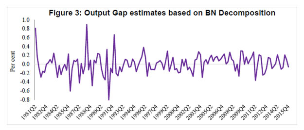 As estimates based on different statistical filters are subject to limitations, it is imperative to estimate potential output using a structural model. Therefore, a Cobb-Douglas production function is estimated using quarterly data on net capital stock and employment. The production function is estimated applying the Fully Modified OLS (FMOLS), proposed by Phillips and Hansen (1990) and Hansen (1992), to avoid bias arising from serially correlated residuals and endogeneity of the variables, particularly when the variables are cointegrated. Further, a test of stability of the parameter is conducted using Hansen’s test and the null of cointegration could not be rejected as the Lc statistic6 was insignificant. The elasticity of output with respect to capital is estimated at 0.61 is highly significant but somewhat higher as compared to other studies. However, the elasticity of capital is comparable to the findings of Ranjan et al. (2007) though almost double as compared to the coefficients assumed by Mishra (2013), Poddar and Yi (2007), and Rodrik and Subramanian (2004) in case of India. The output gap estimates based on production function along with earlier estimates are presented in Figure 4. Production function (PF) based estimates are quite comparable with other estimates but with higher amplitudes of the cycle. The estimate further corroborates the earlier findings on the negative output gap since 2012Q3. However, as compared to other estimates, PF-based estimates suggest a higher negative output gaps during early 1990s and large positive output gaps during 2005-2010. Given the challenge of comparing the relative advantage of one methodology over the other, a composite estimate7 based on principal component analysis that combines all estimates into a single measure is plotted in Figure 5. The figure shows that the output gap was positive during 2005Q2 through 2012Q2 except in 2009Q1, and turned negative since 2012Q3 in the ongoing downturn of the business cycle and was (-)0.6 per cent in 2015Q4. The robustness of different output gap estimates are tested with respect to core inflation. The correlation coefficients of core inflation and output gaps at different lags are estimated and presented in Table 2. The correlation coefficients using Kalman filter based output gap is positive and maximum as the estimation procedure also ensures its consistency with core inflation rate. However, the output gaps estimated using HP one-sided, BN decomposition and CF provide perverse result and may not be considered as suitable estimates. | Table 2: Correlation Coefficients of Core Inflation and Output Gap | | Lags | PF | Kalman | HP two-sided | BK | CF | HP one-sided | BN | Composite | | 0 | 0.13 | 0.31* | 0.10 | 0.10 | -0.21 | -0.31* | 0.01 | 0.16 | | 1 | 0.13 | 0.28* | 0.04 | 0.06 | -0.31 | -0.36* | -0.09 | 0.15 | | 2 | 0.17 | 0.30* | 0.07 | 0.05 | -0.34 | -0.34* | -0.14 | 0.18 | | 3 | 0.26* | 0.38* | 0.17 | 0.11 | -0.27 | -0.24* | -0.02 | 0.27* | | 4 | 0.28* | 0.37* | 0.16 | 0.23* | -0.12 | -0.22** | -0.11 | 0.29* | | 5 | 0.38* | 0.41* | 0.24* | 0.34* | 0.02 | -0.12 | -0.12 | 0.39* | | 6 | 0.45* | 0.47* | 0.33* | 0.41* | 0.10 | 0.01 | -0.07 | 0.47* | | *, **: Significant at 5% and 10% levels, respectively. | The role of capacity utilisation in cyclical fluctuations of output is well documented in real business cycle literature (see Greenwood, et al. 1988; Boileau and Normandin, 1999). Capacity utilisation is expected to have high correlation with cyclical component of output. Therefore, the robustness of output gap estimates are examined considering their correlation with the capacity utilisation8. The correlation between output gap and seasonally adjusted capacity utilisation at different lags and leads are reported in Table 3. As found earlier, output gap estimates based on CF, BN and one-sided HP filters are not representative of the cyclical component of the Indian economy as they have either negative or low correlation with the capacity utilisation. However, PF, Kalman, HP two-sided, BK and the composite measures of output gaps are highly correlated with capacity utilisation and the correlation coefficients are the highest with one lag. Thus, capacity utilisation is a lead indicator of Indian business cycle. | Table 3: Relationship between Capacity Utilisation and Output Gaps | | Lags/ Leads | HP two-sided | BK | CF | Kalman | PF | BN | HP one-sided | Composite | | Lag 0 | 0.71* | 0.74* | 0.45* | 0.77* | 0.76* | -0.47* | 0.31** | 0.78* | | Lag 1 | 0.77* | 0.84* | 0.60* | 0.81* | 0.74* | -0.23 | 0.23 | 0.78* | | Lag 2 | 0.58* | 0.83* | 0.63* | 0.63* | 0.56* | -0.08 | -0.06 | 0.61* | | Lead 1 | 0.59* | 0.57* | 0.20 | 0.68* | 0.75* | -0.31** | 0.35** | 0.75* | | Lead 2 | 0.24 | 0.32** | -0.09 | 0.39** | 0.58* | -0.13 | 0.09 | 0.54* | | *, **: Significant at 5% and 10% levels, respectively. | Another notable thing to be viewed from Figure 6 is that output gap is positive whenever capacity utilisation is around or above 75. Thus, it may be appropriate to say that India’s output attains its potential level when capacity utilisation reaches 75. 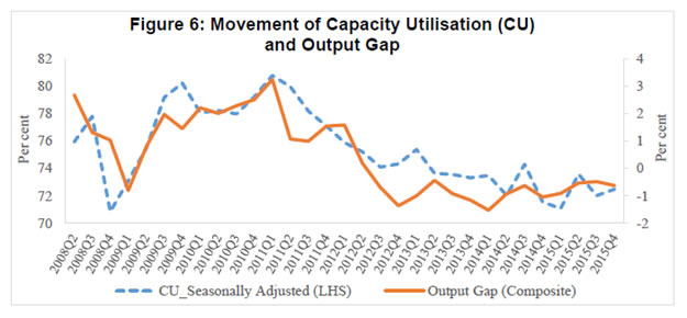 Potential growth is estimated using all those methods employed earlier for the estimation of the output gap. Annualised quarterly growth is calculated from underlying potential output or trend level of output; however, potential growth is directly estimated within the model in case of Kalman filter. In order to provide a representative measure of potential growth, an average of HP-two sided, PF, Kalman and BK based potential growth estimates are considered. Average potential growth is calculated for different periods which are classified looking at broad trend of PF based potential growth and presented in Table 4. The results show that potential growth was low at around 5 per cent during 1981-1991, which increased to around 6 per cent during 1992-2002. But the growth rate accelerated during 2003-2008 and was close to 8 per cent. However, the potential growth had fallen significantly in the post global crisis period and the growth was around 7 per cent during 2009-2015. Most of the estimates suggest that the potential growth is close to 7 per cent at present. | Table 4: Estimates of Potential Growth | | (Per cent) | | Period | Trend | HP two-sided | BK | CF | Kalman | PF | BN | HP one-sided | Represen-tative* | | 1981-1991 | 4.9 | 5.0 | 4.8 | 5.0 | 5.2 | 5.2 | 5.2 | 5.5 | 5.2 | | 1992-2002 | 6.1 | 5.8 | 5.9 | 5.8 | 5.9 | 6.1 | 5.7 | 5.6 | 6.1 | | 2003-2008 | 7.0 | 7.9 | 8.1 | 8.4 | 7.4 | 7.7 | 8.4 | 8.3 | 7.6 | | 2009-2015# | 7.7 | 6.9 | 6.8 | 6.6 | 7.0 | 7.3 | 6.9 | 6.7 | 7.2 | | 2014-15# | 7.9 | 6.6 | 6.8 | 6.8 | 6.8 | 6.7 | 7.1 | 6.3 | 6.7 | #: Covers data up to 2015Q4.
*: an average of the potential growth estimates from HP-two sided, PF, Kalman and BK. | The precise estimates of potential output are difficult to produce and considerable uncertainty is attached to these estimates, mainly related to the methodology, underlying data and judgements about different parameters. However, the uncertainty surrounding the estimates is difficult to measure. An attempt is made in this paper to estimate these uncertainties using Kalman filter. Figure 7 presents the potential growth estimates along with their 95 per cent confidence intervals. According to this estimate, potential growth at current juncture is around 6.8 per cent with a band of (+/-) 50 bps at 95 per cent confidence interval. This implies that the estimates could lie anywhere between 6.3 per cent and 7.3 per cent. The Kalman filter estimates show that India’s potential growth was almost stagnant at around 5.3 per cent till Q3 of 1991, which increased gradually during 1990s and reached 6.2 per cent by end of 2000. The growth amplified thereafter and reached to a peak of 7.6 per cent during 2006-2007 before falling to 6.8 per cent by 2015Q4. As noted earlier also, the potential growth has declined in the post- global crisis period. Factors contributing to this decline in potential growth is examined using production function approach in the following paragraph. 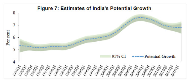 The production function approach adopted in this paper suggests that the medium-term potential output growth is about 7 per cent, and its movement over time is presented in Figure 8. It is important to note that the contribution of capital to output has increased steadily since mid-1990s until 2009, broadly reflecting large capital inflows and pick up in domestic savings contributing to the expansion in domestic capital formation during this period. The contribution of capital stock to growth, which was rising, had fallen since 2010, mainly due to the deceleration in its growth. Additionally, the contribution of total factor productivity (i.e. measured from Solow residual) to overall growth has declined modestly during the recent period9. Between TFP and capital stocks, the fall in the contribution of capital stock to potential growth has been more pronounced. The momentum of growth in the EMEs is mostly driven by investment and therefore, capital formation is a critical factor to sustain high level of growth in the developing countries although contribution of total factor productivity cannot be ignored altogether.  V. Conclusion India’s potential output has been estimated, in this study, using both structural and non-structural estimation techniques for the period 1980Q2 – 2015Q4. According to different estimates, potential growth had increased steadily from its low level of around 5 per cent in 1980s to about 6 per cent during 1992-2002 and accelerated to around 8 per cent during 2003-2008. However, the potential growth fell significantly in the post-global crisis period to around 7 per cent during 2009-2015. The production function analysis further confirms that the potential growth has fallen in the last few years, mainly due to decline in growth of capital stocks and total factor productivity. The semi-structural technique, viz. multivariate Kalman filter, suggests that India’s potential growth for the most recent period is about 6.8 per cent with a band of (+/-) 50 bps at 95 per cent confidence interval. Various estimates of output gap are found to be highly correlated and have identical turning points. All the estimates, except BN, indicate that output gap has been negative since Q3 of 2012, though the gap is closing slowly. Further, the estimated gaps are found to be positively and strongly correlated with core inflation at higher lags, which further confirms the robustness of these estimates. Positive correlation of output gap with the average capacity utilisation further corroborates that output gap could be a good indicator of aggregate demand in India for the policy purpose. Key to accelerate growth as well as potential output in India lies with higher level of capital formation as its contribution dominates vis-à-vis the contribution of labour and the total factor productivity.
References: Anand, R., K.C. Cheng, S. Rehman, and L. Zhang. 2014. Potential Growth in Emerging Asia, IMF Working Paper, No. WP/14/2, January. Baxter, M. and R.G. King. 1995. Measuring Business Cycles: Approximate Band-Pass Filters for Economic Series, NBER Working paper No.5022, Massachusetts. Benes, J., K. Clinton, R. Garcia-Saltos, M. Johnson, D. Laxton, P. Manchev and T. Matheson. 2010. Estimating Potential Output with a Multivariate Filter, IMF Working Paper, No. WP/10/285. Beveridge, S. and C. R. Nelson. 1981. A New Approach to the Decomposition of Economic Time Series into Permanent and Transitory Components with Particular Attention to Measurement of the Business Cycle, Journal of Monetary Economics 7: 151–174. Blagrave, P., R. Garcia-Saltos, D. Laxton and F. Zhang. 2015. A Simple Multivariate Filter for Estimating Potential Output, IMF Working Paper, No. WP/15/79, April. Boileau, M. and M. Normandin. 1999. Capacity Utilization and the Dynamics of Business Cycle Fluctuations, Working Paper No. 99-12, Center for Economic Analysis, University of Colorado, September, url: http://www.colorado.edu/econ/papers/papers99/wp99-12.pdf. Bordoloi, S. A. Das and R. Jangili. 2009. Estimation of Potential Output in India, Reserve Bank of India Occasional Papers, 30(2): 37 – 73. Bosworth, B. and S.M. Collins. 2007. Accounting for Growth: Comparing China and India, NBER Working Paper No. 12943, February. Congressional Budget Office. 2004. A Summary of Alternative Methods for Estimating Potential GDP, Background Paper, March. Cotis, J. P., Elmeskov, J., & Mourougane, A. (2004). Estimates of potential output: benefits and pitfalls from a policy perspective, The euro area business cycle: stylized facts and measurement issues, Centre for Economic Policy Research, 35-60. Christiano, L. J. and T. J. Fitzgerald. 2003. The Band Pass Filter, International Economic Review, 44: 435-465. de Brouwer, G. 1998. Estimating Output Gaps. Research Discussion Paper No. 9809, August, Reserve Bank of Australia. Donde, K. and M. Saggar. 1999. Potential Output and Output Gap: A Review. Reserve Bank of India Occasional Papers. 20(3): 439-467. Goyal, A. and S. Arora. 2012. Deriving India's Potential Growth from Theory and Structure, IGIDR Working Paper, No. WP-2012-018, September. Greenwood, J., Z. Hercowitz and G.W. Huffman. 1988. Investment, Capacity Utilization, and the Real Business Cycle, The American Economic Review,78(3): 402-417. Hansen, B.E. 1992. Efficient Estimation and Testing of Cointegrating Vectors in the Presence of Deterministic Trends, Journal of Econometrics, 53: 87-121. Hodrick, R. and Prescott, E. C. 1997. Postwar U.S. Business Cycles: An Empirical Investigation, Journal of Money, Credit, and Banking, 29(1): 1-16. International Monetary Fund. 2015. World Economic Outlook, April, Washington DC. Mishra, P. 2013. Has India’s Growth Story Withered? Economic and Political Weekly, 48(15): 51-59. Oura, H. 2007. Wild or Tamed?: India’s Potential Growth, IMF Working Paper, No. WP/07/224, September. Phillips, P.C.B. and B.E. Hansen. 1990. Statistical Inference in Instrumental Variable Regression with I(1) Processes, Review of Economic Studies, 57: 99-125. Poddar, T. and E. Yi. 2007. India’s Rising Growth Potential, Global Economics Paper No. 152. New York: Goldman Sachs Global Research Centres. Ranjan, R., R. Jain and S.C. Dhal. 2007. India's Potential Economic Growth: Measurement Issues and Policy Implications, Economic and Political Weekly, 42(17): 1563-72. Reserve Bank of India. 2002. Report on Currency and Finance 2001-02, Mumbai. Rodrik, D. and A. Subramanian. 2004. Why India Can Grow at 7 Percent a Year or More: Projections and Reflections, IMF Working Paper, No. WP/04/118, July. |