Press Release

RBI Working Paper Series No. 01
Estimating Sacrifice Ratio for Indian Economy – A Time Varying Perspective
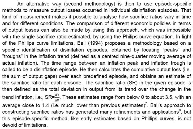
^@Pratik Mitra, Dipankar Biswas and Anirban Sanyal

Abstract

^*This paper estimates sacrifice ratios for the post liberalization period for India. ‘Sacrifice Ratio’ is defined as the loss of output sustained by the economy to achieve reduction in the long-run inflation by one percentage point. Deriving sacrifice ratio by estimating Aggregate Supply Curve has been mostly used across literature. However this framework has been criticized for assuming fixed sacrifice ratio over time. We have tried to address this criticism by using a time varying ARDL framework with transition in parameter and stochastic volatility component. Estimating the model using Gibbs sampling, the sacrifice ratio estimates have increased steadily during expansionary stage of monetary policy and then came down during contractionary period. This paper finds average sacrifice ratio of 2.8 in expansionary phase while 2.3 in contractionary phase.

JEL Classification: E10, E31, E52, E58, E65, C22, C51, C54, C61

Keywords: Sacrifice Ratio, Philips Curve, Okun’s Rule, Time Varying ARDL, Likelihood Estimation, Gibbs Sampling

1. Introduction

The sacrifice ratio is the cost of reducing inflation, the loss of output that must be sustained by the economy in order to achieve a reduction in trend inflation. It is defined as a ratio of the percentage loss of real output to one percent reduction in trend inflation¹. The trade-off between inflation and growth had assumed importance since the Great Depression. Initially during the mid-20th century, focus of the trade-off between inflation and growth was mostly on higher inflation as the cost of higher growth and reduction in unemployment. Friedman (1968) and Phelp (1969) argued that attempt to lower unemployment below its natural rate would only result in higher inflation in the long run. During later part of 1970s and early 1980s, Sacrifice Ratio as a concept, became relevant for developed economies like US where disinflation was considered to be a major cause of recession. US experienced falling inflation scenario resulting out of contractionary monetary policy. Japan also experienced similar phenomenon with slowing growth and falling price for substantial period. In order to discharge its primary responsibility of price stability, the monetary policy authority of a country follows contractionary monetary policy for controlling inflationary pressure. However, such policy achieves its goal of reduction in inflation with an associated cost in loss of output in the interim period. The low inflation regime is believed to have a favourable impact on the economy which might be able to offset the loss of output. In a standard expectation augmented Philips curve framework, for a given potential output level, the reduction in inflation can happen either from moderation in inflation expectation or from the loss of current period output. As expectation takes time to change, the reduction in inflation in the short run is mostly attributed to the moderation in the economic activity. As inflation starts falling over time and if sustained at a lower level, inflation expectation adjusts downwards and the output approaches its potential level. In the long-run, therefore, monetary policy can control and reduce inflation through the inflation expectation channel. As a consequence to this, Phillips curve is vertical in the long-run as the impact of monetary policy on output fades away with time.

Although indisputably the key indicator to understand the real costs of disinflation has been the sacrifice ratio, it has not received due attention in practice mainly due to the lack of reliability of the estimates. A host of empirical studies have estimated the sacrifice ratio and its determinants for various countries, using different econometric methods. Mainly two methodologies have been used in the literature for estimation of sacrifice ratio².

The first estimation method is based on the estimation of the Philips curve, introduced by Okun (1978) and subsequently refined by Gordon and King (1982) who introduced vector auto-regression framework under the assumption of linear Philips Curve. Filardo (1998) introduced non-linearity in the Philips curve by assuming different slope coefficients of the output gap in different phase of the economy.

The second method was introduced by Lawrence Ball (1994). He proposed to use episode-specific method to measure sacrifice ratio. According to the method proposed by Ball, disinflationary episodes are identified based on specific criteria proposed in the paper. Then the total output loss (deviation of actual output from its potential level) during the said episode is calculated by aggregating the output gaps for each time point within the episode. The ratio between the cumulative loss and the reduction in inflation provides the sacrifice ratio for that episode. Relatively detailed exposition of these two methods has been provided later.

In general, it has been observed that the sacrifice ratio estimates vary greatly across countries, episodes (or time periods) and estimation methods. For example, Okun found that the average estimate of the cost of a 1 per cent reduction in the basic inflation rate is 10 per cent of a year’s US GNP, with a range of 6 per cent to 18 per cent. Whereas Gordon and Banks who refined Okun’s approach came up with an estimate of sacrifice ratios that range from 0 to 8, with a mean of about 5. This is just an example of wide variation of the estimates of sacrifice ratio across the method, country and time period. As far as sacrifice ratio of India is concerned, the estimates also vary substantially across the methods. Currency and Finance report of RBI (2002) finds sacrifice ratio as (+2) whereas Kapur and Patra (2003) estimates vary from 0.5 to 4.7 and in some of the cases the estimates were not statistically significantly different from zero. Recently Dholakia (2014) estimated the same as 1.8 – 2.1 (For deliberate disinflationary period) and 2.8 for inflationary period. We have estimated sacrifice ratio for India using these two standard approaches³. Using Ball’s approach and Okun’s aggregate supply curve equation, we observed that the sacrifice ratio estimate varies widely in different disinflationary episodes (Appendix 1). As both these methods have their share of merits and demerits, choosing one over other objectively may not be possible. Ball’s method allows for estimating sacrifice ratio disinflationary episode wise but it does not control for any exogenous shock particularly supply shock⁴. So we can have one disinflationary episode with a strong supply shock impact and another episode without one. If we compare the sacrifice ratio estimated for these two episodes, we get a distorted picture as one of the estimate is highly noisy compared to the other one. Moreover, the dependency on the methodology of potential output estimation also has raised issues on the robustness of the estimate.

On the other hand, the main criticism of the aggregate supply curve estimation method is that it is time invariant. There is no reason to believe that sacrifice ratio for a country would remain the same across time. Also it is widely accepted among the researchers that the sacrifice ratio depends on different factors like speed of disinflation, initial inflation level, trade openness, Central Bank independence to name a few. As these factors change over time, one can safely argue that the sacrifice ratio would also vary over time. This essentially means that the parameters of the short run aggregate supply curve would be time varying. Also as financial crisis period is included in our data, it would be better if we drop the standard homoscedasticity assumption and provide for stochastic volatility. If the different exogenous shocks (mostly supply shocks) are accounted for, this framework would enable us to estimate time varying sacrifice ratio for the period of the study. Taking into account the lack of reliability of the point estimates, we decided to concentrate more on the movement of the estimate over time. Instead of the quantitative measure of the ratio, the qualitative movement of it would help us to carry out a comparative study over time. The movement of sacrifice ratio over the period of study would provide an insight as to how the trade-off between growth and inflation change over time. Dholakia (2014) has argued that one should consider the cases where the monetary policy is involved in a sacrifice of living with higher trend inflation to reduce unemployment and pull people above the poverty line through temporary cumulative income gains. Our method would estimate sacrifice ratio for these period also. So in this paper we try to find answer of the following questions:

1. What is the sacrifice ratio estimate for India in a time varying framework?
2. Qualitatively how the estimates have moved over time?
3. What is the sacrifice ratio estimates for the episodes where policy has induced increase in the long-run inflation rate to gain higher growth of output.

To this end, sacrifice ratio has been estimated using a Philips Curve relationship under time varying⁵ ARDL framework with transition in parameter and stochastic volatility component. This enables us to get time variant sacrifice ratio for the period of the study. Plotting the same over time would provide us a curve which may be termed as ‘Sacrifice Curve’. As Kapur and Patra have underlined the importance of the specification of the short-run aggregate supply function for estimating the sacrifice ratio, we have used the similar specification as used in the Kapur and Patra paper so that the time invariant and time varying estimates could be compared⁶.

Rest of the paper is organized in following manner – Section 2 covers relevant literature review while Section 3 details the data coverage. Sector 4 talks about methodology and empirical findings followed by empirical results and conclusion.

2. Literature Review:

Traditionally the inflation and growth trade-off debate has arguably focused mostly on achieving higher growth and reduction in unemployment at the cost of higher inflation. In this context, the Friedman (1968) and Phelps (1969) critique on the trade-off argued of having a vertical Philips curve in the long-run which signifies that one eventually ends up with only higher inflation and nothing else. The concept of sacrifice ratio in the traditional sense was first introduced by Okun (1978). He estimated a family of Philips curve models to estimate the sacrifice ratio.

This kind of estimation of Philips curve captures the output-inflation trade-off for the given time period. The basic equation is the following Philips curve with adaptive expectations: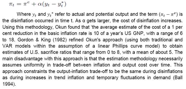

Cecchetti & Rich (2001) criticize Ball's approach for neglecting the impact of supply shocks and other demand shocks (such as money demand shocks or fiscal shocks) on the behaviour of inflation and output during these disinflation episodes. Also they challenged the aggregate supply curve method for not distinguishing the impulse resulting from endogenous impact and policy drift. Accordingly, the Cecchetti & Rich (2001) estimated a generalised Phillips curve relationship through structural vector autoregression models using 2, 3 and 4 variables to get estimates of the sacrifice ratio for the US economy. Although the simplest two variable system of Cecchetti indicates that the true value of the sacrifice ratio may lie somewhere between -0.5 and +3.8, the four-variable system suggests a possible range that extends from -43 to +68. They themselves accept that the degree of imprecision is too high and went on to explore the cause of imprecision.

Turner (1995) and Lactones, et al. (1995) found evidence of non-linearities while estimating Philips Curve for G-7 countries and many other countries including USA. The slope of Philips curve has been found to be steep in case output rises relative to trend. They observed that the non-linearity is sensitive to the nature of Philips Curve and the estimation of output gap. On the other hand, Eisner (1997b) and Stiglitz (1997) reportedly observed evidence favouring concave Philips Curve. Filardo (1998) argued that the sensitivity of output with inflationary changes is dependent on the regimes and hence the functional form depends on the regime.

In Indian context, the first effort to estimate sacrifice ratio traces back to Currency and Finance Report, 2002 (RBI) which stated the estimate of sacrifice ratio as 2. While Kapur and Patra (2003) showed that the sacrifice ratio estimate for India differs depending upon choice of price indicator, time period and specification of short run aggregate supply curve. Their estimate of sacrifice ratio ranged from 0.5 to 4.7 in different time period. This finding was even observed in case of advanced economies like US, Canada, Australia, New Zealand and OECD countries (Kapur and Patra, 2003). In recent times, Dholakia (2014) used direct approach and regression based approach to estimate sacrifice ratio during the time of inflation and forced deflation and his findings ranged from 1.8 to 2.1 for disinflationary period while 2.8 for inflationary period. Estimates of Sacrifice Ratio as indicated in different studies are provided for reference.

3. Our framework

The output – inflation trade-off can be easily illustrated using Expectation Augmented Philips Curve⁹ which can be written as follows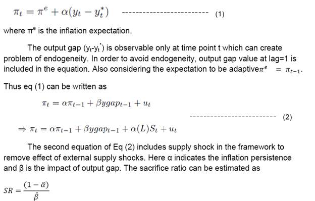

In view of substantial evidence on a possible unit root in inflation¹⁰, the equation can be modified to take inflation in first difference form, following Turner and Seghezza (1999)¹¹. Accordingly, the equation used for estimation is as follows:¹²

However sacrifice ratio defined from Eq (2) and Eq (2.1) necessarily inherits the assumption of constant inflation persistence and output gap impact resulting in constant sacrifice ratio which is questionable considering the economic events in recent times. Particularly, global crisis and subsequent economic downturns question such assumption of constant sacrifice ratio. Also, the sacrifice ratio which typically indicates magnitude of growth sacrifice in order to reduce 1 per cent inflation, is heavily dependent on the initial inflation level and many other factors like Central Bank independence, trade openness, speed of disinflation to name a few (Ball, 1994). So assumption of constant sacrifice ratio may not exhibit changes in the trade-off over different time point. Filardo (1998) indicated that a linear approximation of Philips Curve does not always hold and the shape of the Philips Curve depends upon the regime.

Using aggregate supply curve equation (2.1) in Indian context, we observe that the persistence parameter and output impact are varying widely in different estimation windows using rolling estimation with sliding time window (Chart 1).

In view of the above, we have tried to address the time varying features of parameter estimates using time varying Aggregate Supply curve framework which can be written as follows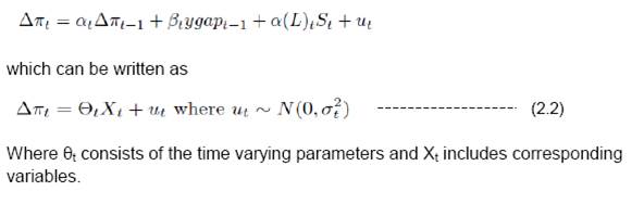

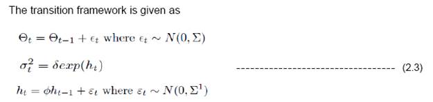
Here we have assumed heteroscedasticity¹³ of residual variance which takes care of the impact of economic turbulences using time varying dynamics.

The framework Eq (2.2) and (2.3) represent state-space representation. The parameter estimation can be performed using maximum likelihood estimation. However the dimensionality of parameter space being large enough, we have used likelihood estimation using multistage Gibbs Sampling technique (proposed by Carter and Kohn 1994). We have used diffused conjugate priors to increase data dependency (in terms of likelihood) rather than prior dependency. We have adopted the methodology suggested by Nakajima (2011) for estimating the model. The convergence diagnostics and auto-correlation checks have been carried out to check the statistical relevance of the estimates.

4. Data Coverage

The aggregate supply curve framework used in this paper uses Philips Curve with adaptive expectation which can be written as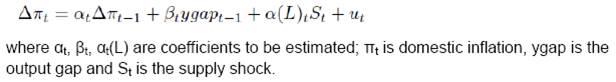

In this paper, WPI Headline inflation has been considered as domestic price indicator while the supply shock components include international price variables and other domestic factors which impacts domestic price. In this line, the supply shock components are listed below –

• International commodity price

• World Food Price provided by IMF
• Metal price indicator (by IMF)
• Indian Basket Crude Oil price

• Domestic variables having impact on domestic inflation

• Exchange Rate movement
• Rainfall

While the pass through of Crude Oil price in international market is well documented in different research papers, we have also considered international food price and metal price to eliminate the pass through of international price into domestic inflation. The exchange rate movement has a positive pass through on inflation (Inflation increases as domestic currency depreciates). Also WPI headline inflation consists of food prices which are influenced by rainfall. Surplus rainfall (IMD Rainfall > 100) corresponds to better agricultural production which tames the food price inflation. Thus the rainfall data has been considered as part of supply shock in our model. Following table lists the transformation and the time period considered

Exchange rate movements have been tracked as Q-o-Q Annualized growth rate as the exchange rate movement does not involve any seasonality. The rainfall indicator has been taken as the deficit rainfall (which is IMD Rainfall Index – 100). Since June-Sept rainfall primarily impacts agricultural production, the average rainfall deficit of June-Sept period has been considered in this context. The rainfall indicator has been used in contemporaneous terms and does not involve any lag.

The output gap has been estimated as

where potential output has been estimated using HP Filter (λ=1600 for quarterly data) after removing the seasonal effects.

5. Empirical findings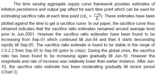

As already mentioned, apart from the disinflationary episodes, this method also covers the period when the policy maker makes deliberate effort to reduce unemployment through temporary cumulative income gains. In such a scenario, sacrifice ratio can be defined as temporary output gain by tolerating 1 per cent increase in inflation¹⁴. In this line, we analyze the sacrifice curve obtained above for expansionary and contractionary episodes. Following graph illustrates the relative level of sacrifice ratio during each of these episodes.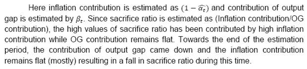

The monetary policy action taken by Reserve Bank can be classified into following episodes –

The grey zones indicate expansionary mode while the yellow zone indicates contractionary mode. The sacrifice ratio is found to be increasing during expansionary mode while it moderates in contractionary mode. Dholakia (2014) also observed that the sacrifice ratio is 2.8 in inflationary period higher than 1.8-2.1 in deliberate disinflationary periods. Our analysis indicate the average sacrifice ratio in each of these episodes as follows.

Since sacrifice ratio is defined as ratio of inflation effect and output impact, we have tried to look at the sacrifice ratio movement in terms of these two effects. The first expansionary period experiences declining output impact along with gradual decline in inflation impact. Since inflation impact is defined as (1-Inflation persistence), the inflation persistence is found to be gradually increasing during this period. Since the output impact (or trade off) came down in a much faster pace sharp increase in sacrifice ratio estimate has been observed. On the same line, the inflation impact was coming down in the contractionary period and output impact remained more or less stable. This phenomenon can be explained in terms of increasing persistence of inflation expectation which kept on dampening the inflation impact.The inflation persistence is found to be declining during the next expansionary phase which resulted in increasing inflation impact. This coupled with stable output gap impact has caused sacrifice ratio to increase in this period. This observation raises question related to persistence of change in inflation during these episodes. In general, the inflation persistence can have direct influence on sacrifice ratio in the sense that higher persistence is followed by small changes in inflation resulting in higher sacrifice ratio. Here we would like to highlight that during this contractionary phase, the persistence coefficient is found to be in the range 0.28 to 0.59 and hence even though the persistence coefficient is gradually going up, the magnitude change of inflation persistence is small in this context.

In this paper, we have also tried to look at the relationship between sacrifice ratio and average level of inflationand average output gap. The average inflation level has been found to be lower when the sacrifice ratio attained peak while the average inflation level was relatively on higher side when the sacrifice ratio was low. This is primarily because the sacrifice ratio is found to be higher in the expansionary phase compared to contractionary phase.

Similar kind of exercise was performed on average output gap which revealed that sacrifice ratio started peaking up when average output gap was at lower level.Butitwas on the lower side when output gap was at higher positive level.

From Chart 5, we observe that the sacrifice ratio estimate is relatively on higher side when the output gap is negative and average inflation level is low and vice versa. As average inflation level is high, the output cost of reducing inflation (which is sacrifice ratio) is low. On the other hand, the output cost of inflation is higher in case the inflation is lower and output gap is negative. Combining these observations, such findings can align to convexity of Phlips Curve (Chart 6)

The convexity of Philips curve ensures that the cost of disinflation is marginal when the total output of the economy is above the trend while the cost of disinflation is expected to rise significantly in case the economy is in recession (i.e. output below the trend output).

6. Conclusion

The output cost arising out of disinflationary steps taken by Central Bank, are mostly confined to interim loses only (Patra and Kapoor (2003)). Every central bank experience such short term loss of output with certain level of inflation expectation and credibility factors. As indicated by wide range of literatures, the estimation of sacrifice ratio is an important assessment for any central bank.

However, it is widely accepted that sacrifice ratio estimate has been found to be varying with choice of estimation methods and potential output estimation method. Even in Indian context, the estimate of sacrifice ratio has been found to be widely varying (Patra and Kapoor (2003)). This paper tries to adopt a time varying approach providing for transition in parameters and stochastic volatility in residual in a way such that the time dynamics can be adequately captured and movement of growth-inflation trade-off can be tracked over time. Using this framework, we observe that the sacrifice ratio estimate is higher during expansionary phase of monetary policy while it comes down in contractionary phase. The highest level of sacrifice ratio was observed in Q3: 2003-04 to Q1: 2004-05 period while it again attained peak during Q1: 2010-11 through a relatively lower level than previous peak value. The movement in sacrifice curve in different episodes depicts the relative contribution of inflation and output.

This paper has focused on the estimation of sacrifice ratio in a time varying framework and tried to address its main criticism¹⁵. One needs to further explore the causality of the movement in the sacrifice ratio.

^@ The authors Pratik Mitra (Email), Dipankar Biswas (Email), and Anirban Sanyal (Email) are Director, Assistant Adviser and Research Officer in the Monetary Policy Department, Financial Markets Operation Department and Department of Statistics and Information Management, Reserve Bank of India, Mumbai respectively.

* The authors are thankful to Mr. Andrew Filardo (BIS) and Dr. Ravindra H. Dholakia (IIM Ahmedabad) and anonymous referee for sharing their comments for enhancement of this paper. Data used in the paper are available in public domain. Views expressed in the paper are those of the authors and not of the organization to which they belong.

¹ In addition to the traditional sacrifice ratio definition, Dholakia (2014) has also considered the period where there is a deliberate effort by the policy maker to reduce unemployment below its natural rate. He has argued that this would involve a similar sacrifice of living with higher inflation permanently to reduce unemployment and pull people above the poverty line through temporary cumulative income gains.

² Apart from the two main methods mentioned above, Cecchetti & Rich (2001) estimated a generalised Phillips curve relationship through structural vector auto-regression (SVAR) models to get estimates of the sacrifice ratio for the US economy. He used three different models of SVAR. But this methodology lost its appeal as it was found out to be grossly imprecise.

³ In Ball’s method, we have tried different variations. Apart from the method prescribed by Ball to estimate potential output, we applied HP filter and the method prescribed by Zhang (2001). As it is widely believed that monetary policy mostly affect the Non-Food manufactured product (NFMP) part of WPI based inflation, we have also tried with NFMP inflation in place of headline. Similarly, on the output side, apart from GDP, we have checked with Non-Agricultural GDP (NAGDP), NAGDP excluding community and social services and GDP-industry. These estimates (provided in Appendix 1) also show similar variations instilling lack of confidence

⁴ Ball (1994) assumes in his paper that shift in demand is the only source of change in inflation. So there is no supply shock. In his sample, he has argued that demand contraction is the main cause of disinflation. However, he has acknowledged that supply shock impact may create this estimate a noisy measure.

⁵ One potential criticism of time varying technique is that the parameter values of Philips Curve relationship may not change in every time point (in this case quarter). Hence instead of looking at parameter value at each time point, we have focused on the average estimates of sacrifice ratio in different episodes and the qualitative movement of the ratio over time period.

⁶ This time varying framework can be extended to other specifications like the one of Dynamic Aggregate Supply and Demand specifications as suggested in Dholakia(2014)

⁷ Ball (1994) applies his episode-specific methodology to 19 OECD member countries using annual data over the period 1960-1991, and then to a sub-group of 9 of these countries using quarterly data over the same period.

⁸ See, for example, Gordan (1997), Neely & Waller (1997) or Zhang (2005).

⁹ The aggregate supply curve framework provides short term trade-off between inflation and output. The medium term aspects are not covered in this framework.

¹⁰ ADF Test reveal presence of unit root in WPI Headline inflation

¹¹ “This specification implies no long run trade-off between the level of output and the level of inflation: a temporary increase in the output gap will lead to a permanent increase in inflation.'; (Turner and Seghezza (1999))

¹² This is the equation used by Patra & Kapur (2003) for estimating sacrifice ratio. Using the same specification would enable us to compare the time varying and time invariant estimates.

¹³ Residual diagnostics of aggregate supply curve framework indicate presence of inter dependency among residual estimates at higher lag which can be considered to be indication of heteroscedasticity.

¹⁴ Unlike the traditional interpretation of sacrifice ratio, higher the sacrifice ratio indicate better trade-off scenario in these episodes.

¹⁵ “The most common approach is to derive the ratio from an estimated Phillips curve-from the relation between output and inflation in a long time-series (Okun 1978; Gordon and King 1982). A limitation of this approach is that it constrains the output-inflation trade-off to be the same during disinflations as during increases in trend inflation or temporary fluctuations in demand” – Ball (1994)

¹⁶ Quarterly estimates prior to 1996 obtained from CSO (from Q1:1990-91 to Q4: 1995-96) and prior to 1990, estimated by Barman et. al. (1994)

References

Akerlof, George, Andrew Rose and Janet Yellen (1988), Comments and Discussion, Brookings Papers on Economic Activity, Vol. 1.

Akerlof, George, William Dickens and George Perry (1996), “The Macroeconomics of Low Inflation”, Brookings Papers on Economic Activity, Vol. 1.

Anderson, Palle and William L Wascher (1999),”Sacrifice Ratio and the Conduct of Monetary Policy in Conditions of Low Inflation”, BIS Working Paper, No. 82.

Bakshi, Hasan, Angrew G. Haldane, Neal Hatch (1997), “Some Costs and Benefits of Price Stability in the United Kingdom”, Bank of England Working Paper, No. 78.

Ball, L., N. Gregory Mankiw and David Romer (1988), “The New Keynesian Economics and the Output-Inflation Trade-off”, Brookings Papers on Economic Activity, Vol. 1.

Ball, L., (1994), “What Determines the Sacrifice Ratio?” in Monetary Policy, edited N. Gregory Mankiw. Chicago: University of Chicago Press, 155-182.

Barro, Robert (1995), “Inflation and Economic Growth”, Bank of England Quarterly Review.

Bomfim, Antulio and Glenn D. Rudebusch (1997), “Opportunistic and Deliberate Disinflation Under Imperfect Credibility”, Board of Governors, Federal Reserve System.

Brumm, Harold J. (2000), “Inflation and Central Bank Independence: Conventional Wisdom Redux”, Journal of Money, Credit and Banking, Vol. 32.

Buiter, Wilem H. and Clemens Grafe (2001), “No Pain, No Gain? The Simple Analytics of Efficient Disinflation in Open Economies”, European Bank for Reconstruction and Development.

Carter, C. K. and R. Kohn, “On Gibbs Sampling for State Space Models”, Biometrika, Vol. 81, No. 3 (Aug., 1994), pp. 541-553

Cecchetti, S. G., and R. W. Rich, (2001), “Structural Estimates of the U.S. Sacrifice Ratio”, Journal of Business & Economic Statistics, Vol. 19, No. 4 (Oct., 2001), pp. 416-42.

Chand, Sheetal K. (1997), “Nominal Income and the Inflation-growth Divide”, IMF Working Paper.

Chortareas, Georgios, David Stasavage and Gabriel Sterne (2002), “Monetary Policy Transperancy, Inflation and the Sacrifice Ratio”, International Journal of Finance and Economics, Vol – 7.

Debelle, Guy and James Vickery, “Is the Philips Curve a Curve? Some Evidence and Implication from Australia”, Reaesrch Discussion Paper, Reserve Bank of Australia, 1997.

Dholakia, H. Ravindra. (2014), “Sacrifice Ratio and Cost of Inflation for the Indian Economy”, Working Paper No. 2014-02-04, Indian Institute of Management, Ahmedabad, February 2014.

Dholakia, H. Ravindra. (2014), “Cost and Benefit of Disinflation Policy in India”, Economic & Political Weekly, Vol xlix no 28, July 12, 2014.

Eisner, Robert,” New View of NAIRU”, in Paul Davidson and Jan A. Kregal, eds, Improving Global Economy: Keynesian and the growth in output and employment. Edward Elgar Publishing Cheltenham: UK and Lyme, U.S., 1997b

Filardo, Andrew J. (1998), “New Evidence on the Output Cost of Fighting Inflation”, Economic Review, Third Quarter, Federal Reserve Bank of Kansas City

Friedman, M. (1968), “The Role of Monetary Policy”, American Economic Review, 58.

Gordon, R. J., (1997), “The Time-Varying NAIRU and its Implications for Economic Policy”, Journal of Economic Perspectives, Winter.

Kapur, M., and M. D., Patra, (2003), “The Price of Low Inflation”, RBI Occasional Papers, Vol. 21, Nos. 2 and 3, Monsoon and Winter, 2000, pp. 191-233.

Mankiw, N. Gregory (2001), “The Inexorable and Mysterious Trade-off Between Inflation and Employment”, The Economic Journal.

Miskin, Fredric S. And Klaus Schmedit-Hebbel (2001), “One Decade of Inflation Targeting in the World: What Do We Know and What Do We Need to Know”, NBER Working Paper no 8397.

Mohanty, D., “Indian Inflation Puzzle”, speech delivered in the function of Late Dr. Ramchandra Parnerkar Outstanding Economics Award 2013 at Mumbai on January 31, 2013.

Nakajima, Jouchi And Toshiaki Watanabe, ”Bayesian Analysis of Time-Varying Parameter Vector Autoregressive Model with the Ordering of Variables for the Japanese Economy and Monetary Policy”, Global COE Hi-Stat Discussion Paper Series gd11-196, Institute of Economic Research, Hitotsubashi University, 2011

Neely, C.J. And C. J. Walter, “A benefit cost analysis of disinflation”, Contemporary Economics Policy, 5, pp. 50-64

Okun, A. M., (1978), “Efficient Disinflationary Policies”, American Economic Review, 68, May.

Phelps, E. (1967), “Phillips Curves, Expectations of Inflation and Optimal Unemployment Over Time”, Economica, 34.

Reserve Bank of India, (2002a), Report on Currency and Finance, 2000-01.

Stiglitz, Joseph E, “Reflections on the Natural Rate”, Journal of Economic Perspectives, Winter, 1997

Turner, D., and E. Seghezza, (1999), “Testing for a Common OECD Phillips Curve”, Economics Department Working Papers, No. 219, OECD.

Zhang, L. H., (2005), “Sacrifice Ratios with Long-Lived Effects”, International Finance, 8(2), pp. 231-262.

Appendix

Appendix 1: Estimation of Sacrifice Ratio in Indian Context
(Using Ball’s Method, Zhang’s method)

Actual developments in output and inflation: In this approach, Ball (1994), Zhang (2005), and H-P filter techniques were applied on quarterly data (Period: Q1:1980-81¹⁶ to Q4:2012-13), for estimating sacrifice ratio. The quarterly GDP data for 1980-81:Q1 to 1995-96:Q4 (at factor cost at 1993-94 prices) was derived from GDP Annual data from corresponding period and segregating the quarterly share using Seasonal factors observed in 1996-97 to 2000-01. During this period, four disinflationary episodes were identified (Table A1). The latest identified disinflationary period is Q2:2000-01 to Q2:2002-03.

The sacrifice ratio estimated using Ball’s method indicate a negative sacrifice ratio for first episode (starting from Q2: 1980) while it is found to be positive but varying widely in the subsequent episodes. On the same line, the estimate of sacrifice ratio is found to be varying widely across episodes using HP Filter and Zhang’s Method. This sort of results raises the question of robustness of assumptions used in Ball’s method and also questions the reliability of estimate. Thus even though Ball’s method incorporates the concept of episode specific estimation of sacrifice ratio, the reliability of estimate can be questionable due to such wide variation.

Further using GDP-Industry, Non-Agriculture GDP (NAGDP), Non-Agriculture GDP excluding ‘Community and social services etc.’ (NAGDP-ex-coss), were used separately as output series, apart from overall GDP. Moreover, apart from Headline inflation, the WPI of Non-food Manufactured Products (NFMP) inflation was also considered for estimating sacrifice ratio (Tables 2 to 5). For NFMP inflation, five disinflationary episodes were identified.