ACKNOWLEDGEMENTS
We thank Development Research Group (DRG), RBI for the
invitation to work on this project, and valuable inputs to progressing it
at various stages. Participants at RBI seminars gave useful comments
where a condensed version was presented. Interactions with RBI officers,
during the course of the project, were a source of rich insights and
contextual knowledge. We are particularly grateful to Dr. Rakesh Mohan,
then Deputy Governor and Dr. Narendra Jadhav, then Principal Adviser
and Chief Economist, Department of Economic Analysis and Policy
(DEAP) for initiating this study, to Dr. Nishita Raje and Dr. Charan Singh,
then Directors, DRG, DEAP for shepherding it through the long process
of completion, to Shri Sanjay Hansda and Shri Ajay Prakash, then
Assistant Advisers, DEAP for initial help and discussions with respect to
the literature review and all DEAP Regional Offices for data support. We
also acknowledge the useful comments of Dr. Laveesh Bhandari of Indicus
Analytics on the first draft, as well as his significant help with the data.
The opinions expressed here are those of the authors and not of the RBI,
or any of the RBI officials acknowledged here. Jake Kendall’s work on
this report was done while he was at University of California, Santa Cruz
and does not reflect the views of the World Bank or any of its affiliated
organizations. The authors are solely responsible for errors and
omissions.
Nirvikar Singh
EXECUTIVE SUMMARY
This study examines regional inequality in India with a particular
focus on data below the state level. There are concerns that regional
inequality in India has been increasing after the economic reforms that
began in 1991. These concerns are supported by several statistical analyses,
conducted mostly with state level data, which, however, does not reveal
anything about what might be taking place within states. More disaggregated
studies are typically qualitative or use only descriptive statistics.
We tackle this gap in analysis by performing a systematic empirical
analysis that admits of some causal interpretation. The main methodology
is the use of cross-section growth regressions, which seek to explain
longer run growth rates in terms of initial conditions of output and
development. In turn, these regressions are derived from, and interpreted
in the light of neoclassical growth theory, which in its basic form, suggests
that diminishing returns to capital accumulation will drive convergence
in income levels across geographic units. We use specific proxy measures
for physical infrastructure, financial development and human capital,
and the regressions identify the connections between these measures
and growth. Hence, the study illuminates the role of aspects of physical
infrastructure, financial development and human capital in influencing
regional patterns of growth below the state level. In turn, this may have
implications for government policies at the national and state levels.
Using region and district level data, we find no evidence for
divergence, but evidence for conditional convergence in some cases. At
the region level, while partial measures of economic activity do not
indicate any strong evidence for conditional convergence or divergence,
there is clear evidence of conditional convergence in per capita
consumption levels. Three points are noteworthy in these results. First,
the convergence result is strongest for urban households. Second, the
main significant conditioning variable is petrol consumption, which could
be an indicator of the quality and quantity of road infrastructure (and
which could also be related to access to urban areas). Third, dummy
variables for the poorer states do not indicate that they were doing worse
than the benchmark average state (Andhra Pradesh), though some of the
regions with the largest negative residuals were in the poorer states.
The district level results also indicate conditional convergence,
but not absolute convergence. The conditioning variables used are
measures of roads, literacy and credit, so the results are supportive of
the importance of infrastructure and human development, as well as
access to finance. These results are quite robust across a wide variety of
specifications, and are consistent with a well-understood model of
development, that emphasizes human capabilities and appropriate access
to markets as determinants of growth. This study can be used to identify
districts which require additional policy intervention along the three
dimensions used, as well as districts where the performance is worse
than the average, even after conditioning on development measures. In
the latter case, social backwardness or policy implementation
shortcomings may be the problem. The results for conditional
convergence hold across states, as well as within most of the states in
the sample, indicating that attention to improving these variables in
districts where they are at relatively low levels can have a growth payoff,
and improve the inclusiveness of growth, as measured by convergence of
income levels across geographic regions.
REGIONAL INEQUALITY IN INDIA IN THE
1990S: TRENDS AND POLICY
IMPLICATIONS
Nirvikar Singh, Jake Kendall, R.K. Jain and Jai Chander*
1. Introduction: Issues and Policy Relevance
There are concerns that regional inequality in India has been
increasing after the economic reforms that began in 1991. These concerns
are supported by several statistical analyses, conducted mostly with state
level data, which show that per capita state domestic products – already
highly unequal – are moving further apart. However, state-level analysis
does not reveal anything about what might be taking place in different
regions within states. On the one hand, the state, as the main subnational
political unit in India, is an appealing level of analysis. Intergovernmental
transfers are decided in terms of allocations to the states, they have
strong cultural identities, and they are strong political units, with
considerable powers assigned to them by the Constitution of India.
On the other hand, states are in some ways too large to allow a full
understanding of regional patterns of economic activity and development.
India’s larger states would rank high among the world’s countries, ranked
by population. Even the medium-sized states have populations larger than
many European nations. Many of India’s states are also quite heterogeneous,
despite strong degrees of linguistic and cultural homogeneity. Within-state
heterogeneity arises in characteristics such as geographic features, degree
of urbanization, infrastructure, and human development. Solely focusing
on differences in economic development across states misses these aspects
of initial conditions and development potential and patterns.
Of course, national government policy has recognized the need to
operate at more decentralized levels. Administrative structures have long
emphasized the district and taluk (block) as significant units of governance.
In the last decade, major constitutional amendments have sought to develop
more autonomous and effective local governments, both rural and urban.
Nevertheless, systematic empirical examinations of regional inequality based
on data below the state level have been extremely limited. This study seeks
to correct this gap in existing empirical analysis, to provide a more finegrained,
quantifiable understanding of trends in regional inequality in India.
In some ways, this analysis fills a key gap between academic analyses
and policy understanding. Policy makers and implementers often have a
deep understanding of conditions at the ground level. Politicians and
bureaucrats operate within their geographic regions of responsibility,
and accumulate considerable local knowledge. Academics have examined
data at the district level in India, but often focusing on description or
summary statistics, rather than formal, empirically-based causal
analysis. Causal analysis has been chiefly aimed at state level data, which
is more easily obtainable. This study therefore uses disaggregated data
to provide an empirical causal analysis that can be instructive for
policymakers at the national and state levels.
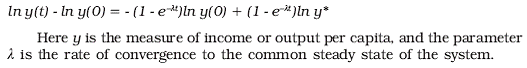
2. Theoretical Framework and Empirical Methodology
Our basic framework comes from the neoclassical economic theory of
growth, which explains growth in terms of factor accumulation. If growth
is expressed in per capita terms, and absent continual technical progress,
diminishing returns to factor accumulation ensure that there is a long
run steady state with constant per capita output, i.e., asymptotically, there
is no growth in per capita output. Thus, economies starting with different
factor endowments will converge to the same steady state, as long as there
are no differences in technologies or other productive opportunities. If,
instead, there is exogenous technological progress, then economies will
grow at the rate dictated by this technological change. Typical neoclassical
growth models (Barro and Sala-i-Martin, 1992, 1995) yield a loglinearization
around the steady state of the form:
 |
If there are persistent differences in technologies, then long run
convergence to a steady state still takes place, but these steady states can
differ, their characteristics being conditional on the differences in productive
potentials. Where faster growth is also affected by other variables besides
initial income levels, the convergence is said to be conditional: in other words,
a poorer country (or region) may converge to a steady state that is different from that of the richer country (or region). Thus, one can identify three
possible scenarios: absolute convergence, where different entities are moving
toward the same steady state, conditional convergence, where they are
converging to (possibly very) different steady states, and divergence, where
there is no evidence of convergence. The last case is inconsistent with
neoclassical growth models, but conceivably fits some endogenous growth
models.1 Note that conditional convergence is quite consistent with increasing
disparities across entities. Variables such as literacy, health and physical
infrastructure may be the conditioning variables, as well as the economic
policies followed. Clearly, the conditioning variables themselves may be
endogenous. However, if one uses these variables at their initial values, they
are predetermined over the growth period being studied, and one can posit
a causal relationship. The empirical implementation of a convergence
regression, allowing for the impact of different initial conditions, then takes
the following form:
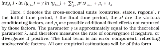 |
Studies of convergence across countries have focused on catching up
by poorer nations through faster growth. While the evidence for any type of
convergence across disparate countries is quite weak, one might expect
greater possibilities for convergence across similar regions or constituent
units of a federation such as India. One problem with this conjecture,
however, is that India itself is extremely large and heterogeneous, and statelevel
convergence regressions, even when restricted to the 14 ‘major’ states,
are subject to some of the same potential shortcomings as cross-country regressions. As will be seen from a review of state-level studies in the next
section, divergence across states may be a serious issue for India. At the
same time, we have relatively little empirical knowledge of how patterns of
growth have been shaping up at the level of geographic regions smaller
than the states.
3. State-Level Convergence Studies
In one of the first studies of convergence within India, Cashin and
Sahay (1996), examined data for the period 1961-91, thus excluding the
reform period of the last decade and a half, but including the Rajiv Gandhi
reform period of the 1980s. The analysis is performed on 20 states, thus
including some of the special category states, which receive central
transfers according to different, and typically much more generous,
formulae than the major states. This is important to note because the
authors use state disposable income per capita, adding in all central
transfers, except for shared taxes, to SDP. They find some evidence for
unconditional convergence in the period of analysis, with the strongest
effect being identified in the 1961-71 decade. These results are not changed
in essence by controlling for other variables. Furthermore, the results
indicate much slower convergence than that found across regions of
developed countries such as the US and Japan. This meant that crosssectional
dispersion of per capita incomes across states actually increased
over the three decades studied, despite the inclusion of center-state
transfers (though dispersion was greater when these were excluded).
Cashin and Sahay also examine the role of internal migration in
convergence, and find it to be weak.
Several analyses followed Cashin and Sahay. Rao and Sen (1997) argue
that the inclusion of four special category states in the Cashin-Sahay sample
muddies their analysis. Furthermore, they argue that adding of transfers to
SDP involves some double counting. Finally, Rao and Sen also take issue
with the analysis of the equalizing effect of transfers, arguing that excluding
shared taxes gives misleading results. Cashin and Sahay’s response, however,
disputes these criticisms on empirical and conceptual grounds. Marjit and
Mitra (1996) independently analyze a data set similar to Cashin and Sahay’s, but with different empirical methods: they argue that the evidence for
convergence is weak. Ghosh, Marjit and Neogi (1998) also find evidence for
divergence across states, over the period 1961-62 to 1995-96.
Nagaraj, Varoudakis and Véganzonès (NVV, 1998) examine data on 17
states for 1970-94 (including three special category states). They find no
evidence for absolute convergence. Using panel data (rather than a crosssection
as in Cashin-Sahay) and per capita SDP (excluding transfers), NVV
find that there is evidence for conditional convergence, with the conditioning
being done on the share of agriculture and the relative price of agricultural
and manufactured goods. Adding infrastructure indicators substantially
strengthens the estimated rate of conditional convergence. While NVV do
not explicitly consider transfers, they emphasize the importance of
infrastructure2 and non-measured political and institutional factors (captured
in state fixed effects) in explaining differences in steady state growth rates
across states. To the extent that center-state transfers have a potential role
in affecting these determinants of growth, they are important in this analysis.
Rao, Shand and Kalirajan (RSK, 1999) examine data for the 14 major
states, for the period 1965-95, using SDP as the output measure. RSK find
evidence for absolute as well as conditional divergence, a result that is
quite robust across sub periods as well. They suggest that the speed of
divergence increased in the last half-decade of their sample. However, this
does not seem to be the decisive factor in explaining the difference from
Cashin-Sahay: instead, the exclusion of special category states, and of centerstate
transfers are of greater importance. The differences in conditioning
variables and estimation methodology from NVV (who use a fixed-effects
panel model) may explain the difference in conditional convergence results
between RSK and NVV. RSK emphasize the role of private investment in
explaining growth differences across states. They find that private
investment goes disproportionately to higher-income states, as well as to
states that have higher per capita public expenditures.3 RSK also argue that explicit center-state transfers have had moderate impacts on interstate
inequalities, and that these effects have been outweighed by implicit
transfers through subsidized (public and private) lending and through
interstate tax exportation.
Two other similar studies of possible convergence among India’s states
are those of Bajpai and Sachs (1999) and Aiyar (2001). The former study
examines data for a sample of 19 states for 1961-93. For the sub-period
1961-71, they find some evidence of convergence, but not for later subperiods
or for the period as a whole. Allowing for conditional convergence
does not qualitatively alter these results. Aiyar also uses the 19-state
sample, for 1971-96. He finds weak evidence of absolute convergence for
the 1970s, but divergence for later sub-periods (especially the 1990s), as
well as for the overall period. He estimates a panel with fixed effects, as
do NVV, in which he does find evidence of conditional convergence. His
conclusions are similar to those of NVV and RSK, emphasizing the
importance of infrastructure, private investment, and non-measured
institutional factors.
Singh and Srinivasan (2005) examined the effects of foreign direct
investment (FDI), as well as credit availability, in state-level convergence
regressions (Table 1). They obtain several interesting results. First, the
evidence for convergence or divergence is inconclusive, since the coefficient
of base-year SDP is never significantly different from one.4 Second, any
one of the financial variables taken individually is estimated to have a
significant impact on growth of SDP. When two or more financial variables
are included, there is evidence of multicollinearity, but otherwise the results
are robust. They are consistent with a story where domestic and foreign
capital are complements, and with data on credit-deposit ratios and of FDI
approvals (both suggesting greater regional concentration of credit and
investment),5 the evidence is suggestive of mobile domestic and foreign
capital driving growth.
Table 1: State Level Growth Regressions |
Dependent variable is log of 1998-99 per capita SDP
(t-statistics in parentheses) |
Variable |
(1) |
(2) |
(3) |
(4) |
(5) |
(6) |
(7) |
Constant |
-0.86 |
-0.02 |
-0.70 |
-1.16 |
0.13 |
0.84 |
1.18 |
|
(-0.94) |
(-0.02) |
(-0.76) |
(-1.65) |
(0.11) |
(0.79) |
(1.12) |
1990-91 ln SDP |
1.14 |
1.02 |
1.08 |
1.14 |
0.96 |
0.90 |
0.85 |
per capita |
(9.75) |
(9.79) |
(9.71) |
(12.71) |
(6.41) |
(6.21) |
(5.95) |
FDI approvals |
|
5.4E-05 |
2.4E-05 |
|
6.3E-06 |
3.3E0-5 |
|
p. c. 1991-2001 |
|
(2.76) |
(0.81) |
|
(0.19) |
(1.25) |
|
Credit-deposit |
|
|
0.35 |
0.52 |
0.33 |
|
|
ratio 1990 |
|
|
(1.34) |
(3.10) |
(1.26) |
|
|
Credit per |
|
|
|
|
8.9E-05 |
9.7E0-5 |
16.6E-05 |
capita 1990 |
|
|
|
|
(1.12) |
(1.19) |
(2.71) |
Adabar (2005) uses data for the 14 major states of India from 1976-77
to 2000-01 and employs a dynamic fixed effects panel growth regression.
Once per capita investment, population growth and human capital, along
with state-specific effects are controlled for, he finds evidence of conditional
convergence at the rate of about 12% per five-year span. Purfield (2006) also
uses dynamic panel estimates with data for the 15 largest states for 1973/
74–2002/03 (averaged over six non-overlapping five-year periods). She finds
slow absolute convergence, somewhat faster conditional convergence, and,
somewhat surprisingly, negative impacts on growth of the size of state
government.6 Some of the other results are also puzzling, illustrating the
difficulty of reaching definitive conclusions with state-level data.
4. Inter-State Inequality in India: Additional Perspectives
Ahluwalia (2000) examines the most recent data on the performance
of India’s states. He uses the Gini coefficient for the 14 major states, and
finds that interstate inequality, after being stable for most of the 1980s,
increased, starting from the late 1980s, and even more in the 1990s. Many
of the factors that he identifies as affecting growth performance are those
emphasized earlier by NVV and RSK, suggesting that the fundamental situation that India faced earlier in the reform period has persisted through
the decade of the 1990s.7 Ahluwalia (2001) adds some simple regressions
to his earlier analysis, but these do not change the overall analysis or
conclusions.8
Dasgupta et al (2000), covering a period from 1960-61 to 1995-96,
find a clearly diverging pattern amongst the states in terms of the coefficient
of variation of per capita SDP as also the growth in per capita SDP. In
terms of the rank correlation matrix (in respect of per capita SDP) as also
the index of rank concordance, the position of states turned out remarkably
stable for any chosen pair of years. The sectoral contribution, viz., from
primary, secondary and tertiary sectors, to the overall divergence indicates
that the divergence between states is least in terms of infrastructural
development and largest with respect to agriculture. Considering the
structural features defined in terms of sectoral shares, this study has,
however, brought out a case against divergence.
Based on a careful review of a multitude of factors relating to
demographic indicators, female literacy, SDP, poverty, development and
non-development expenditure by state government, shares in plan outlay,
investments, banking activities and infrastructure development, Kurian
(2000) argues that the accelerated economic growth since the early 1980s
with increased participation by the private sector has aggravated regional
disparities. The ongoing economic reforms since 1991, with stabilization
and deregulation policies as their prime instruments and a very significant
role for the private sector, seem to have further accentuated the disparities.
By using a non-parametric kernel density for poverty estimation,
Dhongde (2004) decomposes the changes in poverty across regions for the
year 1999-00 and observes that differences in state and national poverty
levels were largely explained by differences in the state and national mean
income levels rather than differences in the state and national distributions of income. An important policy implication of the study is that states with
extremely high levels of poverty would have reduced poverty significantly
by raising their mean income levels to the national mean income, instead
of changing their distribution of income to match the national income
distribution. In other words, growth toward the average income level is
more important for poverty reduction than redistribution toward the average
distribution.
Lall and Chakravorty (2004) suggest that spatial inequality of industry
location is the primary cause of spatial income inequality in developing
nations. In this context, the contribution of economic geography factors to
the cost structure of firms in eight industry sectors in India was examined
and the local industrial diversity was found to have significant and
substantial cost reducing effects. Since new private sector industrial
investments in India are biased toward existing industrial and coastal
districts while state industrial investments (in deep decline after structural
reforms) are far less biased toward such districts, the study concludes
that structural reforms lead to increased spatial inequality in
industrialization, and therefore, in income.
Dholakia (2003) has examined the trends in regional disparity in
economic and human development in India over the last two decades. His
study points out that while per capita income does not show any significant
trend in regional disparity over the last two decades, seven out of nine
human development indicators display a declining trend in regional
disparity. Similarly, 12 of the other 16 related social and human
development indicators show a marked decline in regional disparity during
1981-91. The concept and measurement problems involved in Indian data
on state domestic product are briefly discussed in Dholakia (2003) to point
out the limitations of past studies on the subject. In a cross-sectional setting,
Granger causality or precedence is tested by considering lags in the
independent variable and interchanging the variables. Using this method,
Dholakia (2003) finds a two-way causality between human and economic
development. The structure of the relationship was found to be varying
over time when human development indicators (HDIs) are the cause and
per capita SDP is the effect, but in the reverse causality case, the structure of the equations is stable over time. Moreover, HDIs have been found to
positively influence per capita SDP with a lag of about eight years, whereas
per capita SDP affects the HDIs within two years. Therefore, according to
this analysis, emphasis on economic growth is likely to address the issue
of twin disparities in income and human development in the shortest time.
This analysis also suggests that emphasis on human development in states
may lead to the postponement of rapid economic growth and also to some
inefficiencies cropping up in the delivery of output, resulting in a further
shifting of the structure of relationship between per capita SDP (effect) and
HDIs (cause).9
Jha (2000) examines the empirical relationship between economic
inequality, poverty and economic growth in the Indian states. Gini coefficient,
real mean consumption and the head count ratio for rural and urban sectors
and average for 14 major Indian states has been computed using NSS data
on consumption for the 13th to the 53rd Rounds. The study finds that
there is (conditional) convergence (in terms of levels) in inequality and
poverty measures across states. The coefficients of variation do not show
any tendency to fall over time. Based on the observation of a rising coefficient
of variation of the rural head count ratio, the study points towards greater
dispersion in rural poverty across states over time. Inequality was found
to be acting as a constraint on growth in the states with high Gini coefficients
as well with poor growth performance. Therefore, the author recommends
that economic growth should be used for reduction of inequality and poverty.
For equitable distribution of consumption, he suggests widespread tax
reform to increase tax revenues and economic growth and make the tax
structure more redistributive; improvement of efficiency of public
expenditure and of the social safety net; and design of a good social sector
policy framework promoting agricultural growth as opposed to nonagricultural
growth, protecting the poor from the effects of macroeconomic
shocks and building up of pressure groups of the poor.
5. Regional Inequality: Disaggregated Studies
Kurian (2000) has examined intra-state disparities and drawn attention
to the fact that the newly created states develop faster than the pre-partition
states. The study highlights a few successful cases where intra-state regional
disparities were reduced considerably through public policies such as in
Malabar region (Kerala), drought-prone districts of Haryana and the remotest
villages of Himachal Pradesh. Tamil Nadu was identified as the most
successful state in reducing intra-state disparities even with substantial
variation in natural endowments across different parts of the state.
In an attempt to estimate the district health accounts in Karnataka
for the year 1997-98, Annigeri (2003) observes that in terms of sources
of funds, private funds account for about 52 per cent of the resources
flowing into the district. Interestingly, both state and union governments
are found to have spent less on medicines than on salary.
Gulmoto and Rajan (2002) have provided district level indirect
estimates of birth and fertility rates for all districts of India using population
aged 0-6 years as observed in 2001. While the fertility is lower than 3
children per woman for the southern and coastal states along with Punjab,
Himachal Pradesh, Tripura and Manipur, high fertility districts (i.e., with
more than 5 children per woman) are still widespread in north India.
Nonetheless, there is evidence to believe that India is passing through the
last phase of fertility transition, moving towards moderate to low fertility.
Debroy and Bhandari (2003) identify 69 backward districts based on six
indicators, viz., poverty ratios, hunger, infant mortality rate, immunization,
literacy rate and enrollment ratios. Sources of data include both primary and
secondary sources. Each indicator throws up a set of districts. Based on poverty
ratios, they find that backward districts are present, apart from the BIMARU
states (Bihar, Madhya Pradesh, Rajasthan and Uttar Pradesh),10 in Gujarat, Maharashtra, Karnataka, Tamil Nadu, Andhra Pradesh, Orissa, West Bengal
and the North-East. Hunger has a similar spatial distribution with less
universality and more concentration in the East and the North-East. Backward
districts based on infant mortality rates are concentrated in the BIMARU
states and Orissa with some presence in Karnataka and Andhra Pradesh.
Lack of immunization was found to be prevalent in the BIMARU states.
Districts with low literacy rates and enrollment ratios are found to be spread
all over the country. Given that each indicator selected a different set of
districts, a backward district has been defined by them as one which is
backward as per four out of the above six indicators. The 69 districts so
identified are distributed as follows: 26 in Bihar, 13 in UP, 10 each in
Jharkhand11 and Orissa, 6 in Madhya Pradesh, 3 in Arunachal Pradesh,
and 1 in Karnataka.
Debroy and Bhandari (2003) observed that connections between 69
backward districts and the rest of the economy are grossly inadequate,
with poor national highways, state highways and railway networks. Poor
infrastructure deters the private sector, making development dependent
on public funds. Flood problems in Bihar, UP and Orissa are also considered
as the cause for their backwardness. Thus, addressing these two issues
among others is crucial for uplift of these backward districts. As we shall
see in subsequent sections, our district-level analysis provides a quantitative
analysis of the the linkages informally explored by Debroy and Bhandari.
Using the estimation procedure of the NSS 55th round on variables
for monthly household consumer expenditure and household size, Sastry
(2003) has made district level poverty estimates, and shows that it is feasible
to derive valid distributions for a majority of districts on the basis of Relative
Standard Errors criteria. Finally, Singh et al. (2003) use NSS region level
data to examine issues of convergence, though performance has to be
measured by alternatives to income, which is not available at this level of
disaggregation. This kind of data forms the basis for part of our analysis,
and is discussed further in the next section.
6. Data Description and Summary Indicators
We use two sets of data for the analysis conducted in this report. First,
we use data from the National Sample Survey (NSS), which is at the level
of agro-climatic regions. There are 78 such regions in India, but we have
complete data for 59 regions, which forms the basis for the analysis here.
This analysis extends the work of Singh et al (2003). The data used here
include six variables: consumption expenditure, petrol sales, diesel sales,
bank credit, bank deposits and cereal production. Consumption
expenditure provides the broadest measure of economic activity among
these. There are issues with respect to differences in data collection
methodology across rounds, but we believe the analysis is still valid. In
particular, since we are examining cross-sectional variation in growth rates,
rather than time trends, data collection methodology changes are less
important, and less likely to be a source of bias.
The most novel aspect of the analysis performed here is the use of
district level data to conduct a convergence analysis of growth. We use
data on district level domestic product (DDP), along with data on
population, road kilometers, literacy rates, and credit and deposit levels.
DDP data was obtained from individual state governments, credit and
deposit levels from RBI regional offices, and the other variables from the
Indian Census. The main data constraint was in availability of DDP data,
and this restricted us to nine states. The relevant states are highlighted
in Table 2, with some summary statistics. The nine states covered account
for over 60 percent of the country’s population and domestic product.12
The sample states are on average slightly above the national average per
capita NSDP. There is also some regional variation in the sample, although
with relatively greater coverage of the southern states (4), followed by
northern states (3) and one each from the west and east. Maps of the
states with districts named as in 1991 are shown in Appendix 1. The
data used are for 1991 and 2001, allowing a ten-year snapshot of growth
across the districts in our sample.
Table 2: Basic Characteristics of States (2001) |
|
Area
(Sq. Km) |
Population
(in ‘000) |
Density
of Popn. |
NSDP
1999-00
Rs.
Million |
Per capita
NSDP
(1999-00) |
Percentage
of Total
Area |
Percentage
of Total
population |
Percentage
of Total
NSDP |
Andhra Pradesh |
275000 |
75728 |
275.4 |
1117530 |
14878 |
8.36 |
7.37 |
7.9 |
Bihar |
94000 |
82879 |
881.7 |
383260 |
4813 |
2.86 |
8.07 |
2.71 |
Chhattisgarh |
135100 |
20796 |
153.9 |
213310 |
10405 |
4.11 |
2.02 |
1.51 |
Goa |
3800 |
1344 |
353.7 |
58620 |
44613 |
0.12 |
0.13 |
0.41 |
Gujarat |
196000 |
50597 |
258.1 |
896060 |
18685 |
5.96 |
4.93 |
6.33 |
Haryana |
44000 |
21083 |
479.2 |
424880 |
21551 |
1.34 |
2.05 |
3 |
Jharkhand |
79700 |
26909 |
337.6 |
232270 |
9223 |
2.42 |
2.62 |
1.64 |
Karnataka |
192000 |
52734 |
274.7 |
862980 |
16654 |
5.84 |
5.13 |
6.1 |
Kerala |
39000 |
31839 |
816.4 |
569260 |
17709 |
1.19 |
3.1 |
4.02 |
Madhya Pradesh |
308000 |
60385 |
196.1 |
677780 |
11626 |
9.37 |
5.88 |
4.79 |
Maharashtra |
308000 |
96752 |
314.1 |
2131510 |
22604 |
9.37 |
9.42 |
15.07 |
Orissa |
156000 |
36707 |
235.3 |
311950 |
8733 |
4.75 |
3.57 |
2.21 |
Punjab |
50000 |
24289 |
485.8 |
554700 |
23254 |
1.52 |
2.37 |
3.92 |
Rajasthan |
342000 |
56473 |
165.1 |
710200 |
13046 |
10.4 |
5.5 |
5.02 |
Tamil Nadu |
130000 |
62111 |
477.8 |
1143090 |
18623 |
3.95 |
6.05 |
8.08 |
Uttar Pradesh |
241000 |
166053 |
689 |
1493520 |
9323 |
7.33 |
16.17 |
10.56 |
Uttarakhand* |
53500 |
8480 |
158.5 |
na |
na |
1.63 |
0.83 |
0 |
West Bengal |
89000 |
80221 |
901.4 |
1175070 |
14874 |
2.71 |
7.81 |
8.31 |
Special |
|
|
|
|
|
|
|
|
Category States |
540500 |
55182 |
102.1 |
639300 |
12339 |
16.44 |
5.37 |
4.52 |
All States |
3276600 |
1010562 |
308.4 |
13595290 |
14359 |
99.67 |
98.4 |
96.11 |
UTs |
10974 |
16453 |
1499.3 |
549870 |
31211 |
0.33 |
1.6 |
3.89 |
States in Sample |
1719500 |
654680 |
380.7 |
9757860 |
14905 |
52.3 |
63.75 |
68.98 |
Total |
3287574 |
1027015 |
312.4 |
14145160 |
13778 |
100 |
100 |
100 |
Source : Rao and Singh, 2005,
Table 4.1
* Uttarakhand is technically included in Uttar Pradesh for the decade analyzed, but the districts comprising
it are not in our sample. |
There are issues of comparability across states in DDP data, but this
is addressed to some extent by analyzing the data state by state (in addition
to pooling across states). Indira et al. (2002) looks at the ‘far from settled’
conceptual and availability issues of data on income and poverty estimates
at the district level. It is based on discussions at a UNDP sponsored
workshop in July 2001 to develop a common methodology for calculation
of district level income and poverty estimates. Some issues that were
debated and discussed are as follows. While some states limit district income to commodity producing sectors (‘district product’) others include
non-commodity producing sectors as well (‘district income’). Animal
husbandry needs to be clubbed with agriculture. District level prices need
to be developed. Estimation of services is very difficult due to no estimates
of income accrued in a district. Remittances from another state need to be
distinguished from remittances from abroad. Thus, for various conceptual
differences, DDP across states may not be strictly comparable. Issues
relating to the definition, database and methodology to be used for
estimation of poverty at the district level are also far from settled.
Despite the data comparability and other measurement issues, we
would argue that district-level analysis still has validity. Certainly, individualstate
regressions avoid issues of comparability across states. To some extent,
comparability can also be handled by including state dummies in pooled
regressions. Overall, we would argue that even imperfect measurement is
better than none at all, and to the extent that biases in data can be identified,
one can also point out potential biases in the results. Methodologically, it
is also worth noting that measurement error in the dependent variable
(here, DDP, which is most subject to data problems) does not lead to biased
coefficients, only to greater imprecision. The omission of relevant
explanatory variables in the regressions may therefore be a greater practical
source of bias.
7. Analysis of NSS Regional Data
The NSSO divides the Indian states into 78 homogenous agro-economic
regions that are groups of contiguous districts, demarcated on the basis of
agro-climatic homogeneity. Each region is contained within a state or union
territory. Together these regions cover all of India. For each region, Bhandari
and Khare (2002) constructed an economic performance index based on
five variables: petrol sales, diesel sales, bank credit, bank deposits and cereal
production. They compared the years 1991-92 and 1998-99, and reported
how each region did over this period, in terms of share of the overall economy.
The Bhandari-Khare calculations revealed several interesting patterns.
First, a clear West-East divide emerges in their analysis, with the West increasing its economic share. Second, there is no obvious North-South or
coastal-inland divide. Third, most of the regions that do the best are centered
on urban areas, which appear to be acting as growth poles. Fourth, many
of the areas that lag are rain-fed agricultural regions, consistent with the
general consensus that agriculture has been bypassed by the reform
program to date.13 Fifth, Punjab, Haryana and Kerala do relatively well in
this analysis (better than when per capita SDP is used as a measure of
performance), consistent with a possible impact of international remittances
for these states. Finally, while some states are doing consistently well, in
terms of all regions within the state increasing their relative share (e.g.,
Karnataka, Kerala, Punjab and Haryana), there are other states with marked
internal disparities in regional performance (e.g., Andhra Pradesh, Madhya
Pradesh and Maharashtra). Thus, going down to the NSS region level
provides a considerably more nuanced picture of the geographic patterns
of economic change in the post-reform period.
Singh et al (2003) performed convergence analysis using the five
individual components (diesel consumption, petrol consumption, credit,
deposits, and cereal production) of the Bhandari-Khare index. Due to data
gaps, 59 of the NSS regions were used for the regressions, covering all the
14 major states, plus Assam and Himachal Pradesh. Thus, the coverage at
the region level exceeds what we are able to achieve in subsequent sections
at the district level, which, on the other hand, provides greater disaggregation.
Therefore, this tradeoff further justifies analysis at both levels. In the absence
of dummies, growth of credit and diesel consumption show evidence of
absolute divergence, while only the latter result persists when conditioning
variables are included. Including zonal dummies for north, west and south
completely removes any absolute or conditional divergence effects, but the
three zonal dummies are all statistically significant (except in the case of
cereal production), indicating otherwise unexplained differences in the growth
processes across these zones of the country.
Here we present a more detailed examination of interstate variation by
including state level rather than zonal dummies. Andhra Pradesh is used as
the base state, and its dummy variable is therefore omitted. The results are
summarized in Table 3, with standard errors reported in parentheses below
coefficient estimates. Statistically significant positive and negative coefficients
(excluding the constant terms) are marked in blue and yellow respectively
with asterisks. Of the five variables used to measure economic activity, two,
namely petrol consumption and cereal production (each in per capita terms),
indicate statistically significant evidence of conditional convergence. In each
of the regressions, none of the economic variables used for conditioning are
statistically significant, indicating that the initial conditions that influence
growth performance are not being captured in this data set.
The chief variables of interest, however, are the state level dummies.
In a cross-section regression with state-level data, there is limited scope to
include such dummies. Here, we are able to examine the entire pattern of
base-level growth differences across the states with dummies. We use
Andhra Pradesh as the control state, as it is a state with an intermediate
growth performance in the period under examination. Hence, each state
dummy represents growth performance compared to Andhra Pradesh,
controlling for all measurable effects with the data available. According to
this criterion, we see that Assam, Orissa and Bihar are by far the worst
performers among the states in the sample. All these states are in Eastern
India. Orissa has statistically significant (at least at the 5% level) negative
coefficients for all five of the variables, while the other two states have
statistically significant coefficients for four of the variables – excluding
deposits for Assam and cereal production for Bihar – though in each case
the coefficients are still negative.
For each of Madhya Pradesh, Rajasthan and Uttar Pradesh, petrol
consumption and credit are both negative and significant. Diesel and petrol
consumption are both negative and significant for West Bengal. Gujarat,
Haryana and Maharashtra each have a single negative and significant dummy
coefficient among the five regressions, without any positive and significant
coefficients. In the case of Kerala, the dummy in the cereal production
regression is negative and significant, while the coefficient for the petrol consumption regression is positive and significant. The only other positive
and significant coefficients are for Punjab in the cereal production
regression, and for Himachal Pradesh in the diesel and petrol consumption
regressions and the deposits regression. Overall, therefore, the picture that
emerges from these regressions is consistent with the view of the Eastern
states and the BIMARU states as the worst performers in terms of economic
growth. The caveat to this observation is that each individual performance
measure only provides a very partial indicator of economic activity.
Table 3: Regional convergence of development indicators
convergence of development indicators
with state dummies |
Dependent Variable Independent Variable |
Diesel Consumption |
Petrol Consumption |
Deposits |
Credit |
Cereal Production |
Constant |
0.2776 |
0.2093 |
0.5190 |
0.6987 |
-0.2060 |
|
(0.1593) |
(0.1075) |
(0.1537) |
(0.1848) |
(0.4525) |
Diesel Cons. 1991 |
-0.1086 |
0.1374 |
-0.0853 |
-0.1672 |
-0.1248 |
|
(0.1160) |
(0.1038) |
(0.0720) |
(0.1084) |
(0.2100) |
Petrol Cons. 1991 |
0.0589 |
-0.1619*** |
-0.0068 |
0.1281 |
-0.1474 |
|
(0.0521) |
(0.0446) |
(0.0478) |
(0.0770) |
(0.1515) |
Deposits 1991 |
-0.0345 |
-0.0273 |
0.0288 |
0.0492 |
0.0426 |
|
(0.1132) |
(0.0460) |
(0.0791) |
(0.1111) |
(0.3845) |
Credit 1991 |
-0.0235 |
0.0210 |
-0.0704 |
-0.0778 |
0.0347 |
|
(0.1184) |
(0.0526) |
(0.0818) |
(0.1173) |
(0.3953) |
Cereal 1991 |
-0.0183 |
0.0458 |
-0.0437 |
-0.0619 |
-0.2847** |
|
(0.0459) |
(0.0471) |
(0.0410) |
(0.0536) |
(0.1373) |
Assam |
-0.6696*** |
-0.5985*** |
-0.1406 |
-0.4087*** |
-0.6953* |
|
(0.1223) |
(0.0767) |
(0.1029) |
(0.1310) |
(0.3473) |
Bihar |
-0.3547*** |
-0.5282*** |
-0.3489*** |
-0.5541*** |
-0.5945 |
|
(0.1149) |
(0.0686) |
(0.0954) |
(0.1520) |
(0.3907) |
Gujarat |
0.1698 |
-0.0200 |
0.0578 |
-0.2135** |
-0.5650 |
|
(0.1185) |
(0.0501) |
(0.0900) |
(0.0919) |
(0.4086) |
Haryana |
0.1276 |
-0.3456** |
0.0706 |
-0.1790 |
0.4168 |
|
(0.1337) |
(0.1507) |
(0.1202) |
(0.1675) |
(0.2858) |
Himachal Pradesh |
0.6252*** |
0.3600*** |
0.5864*** |
0.0254 |
-0.0520 |
|
(0.1342) |
(0.0736) |
(0.1126) |
(0.1361) |
(0.4212) |
Karnataka |
0.0493 |
-0.0489 |
0.1638 |
-0.0284 |
0.0651 |
|
(0.0823) |
(0.0683) |
(0.0911) |
(0.1109) |
(0.2400) |
Kerala |
0.0231 |
0.1915** |
0.1963 |
-0.0790 |
-0.8768*** |
|
(0.0865) |
(0.0799) |
(0.1028) |
(0.1086) |
(0.2991) |
Madhya Pradesh |
-0.1876 |
-0.3006*** |
-0.1035 |
-0.2463** |
-0.0747 |
|
(0.0999) |
(0.0519) |
(0.0840) |
(0.0968) |
(0.2139) |
Maharashtra |
-0.1098 |
-0.1612*** |
0.0207 |
-0.1112 |
-0.4939 |
|
(0.0585) |
(0.0451) |
(0.0882) |
(0.1043) |
(0.2681) |
Orissa |
-0.2371** |
-0.2124** |
-0.5022** |
-0.8034*** |
-0.4095** |
|
(0.1173) |
(0.0869) |
(0.1980) |
(0.1988) |
(0.2049) |
Punjab |
0.0815 |
0.0054 |
-0.0547 |
-0.2224 |
0.8912** |
|
(0.1691) |
(0.1523) |
(0.2010) |
(0.2565) |
(0.4081) |
Rajasthan |
0.0441 |
-0.1580** |
-0.0864 |
-0.2180* |
-0.2098 |
|
(0.1061) |
(0.0732) |
(0.0783) |
(0.1087) |
(0.2334) |
Tamil Nadu |
0.0524 |
0.1431 |
0.1373 |
0.1390 |
0.1361 |
|
(0.0597) |
(0.1126) |
(0.0708) |
(0.0821) |
(0.2140) |
Uttar Pradesh |
-0.1948 |
-0.3985*** |
-0.1516 |
-0.4706*** |
-0.2176 |
|
(0.1032) |
(0.0567) |
(0.0988) |
(0.1156) |
(0.3798) |
West Bengal |
-0.2256** |
-0.5017** |
-0.1497 |
-0.1796 |
-0.1208 |
|
(0.0908) |
(0.0573) |
(0.0901) |
(0.1061) |
(0.3121) |
Note: Standard errors are in parentheses. ***p<0.01, **P<0.05, *p<0.1 |
Further understanding of the growth performance of regions comes
from examining the residuals for the different regressions. Table 4
summarizes the five best and worst performing regions in terms of
magnitudes of negative residuals. A large negative residual indicates that a
region does worse than would be predicted by the explanatory variables in
the regressions. There is some degree of pairing among regions within
states, for best and worst regions. This is a consequence of the inclusion of
state level dummies in the regressions. However, the presence of certain
states and not others within these extreme residuals is perhaps indicative
of greater disparities within these states relative to other states. Other
possible factors are the size of the state (larger states being more
heterogeneous, with more regions) and greater heterogeneity independent
of size (e.g., Maharashtra may be especially heterogeneous in terms of
urbanization and climatic variety). Perhaps the most important observation
is to note that some regions are among the worst performers, even
controlling for the states they are in. In particular, Orissa is the worst
performer in terms of credit and deposits, with the largest negative dummy
coefficients, and Coastal Orissa is the worst performer, even beyond the
state average. Other cases of extreme outliers appear to be Southern Orissa
for diesel consumption, and Western Haryana for petrol consumption.
We also have data on personal consumption expenditure from the
50th and 55th rounds of the NSS, for rural, urban and all households.14 While
these data are for 1993-94 and 1999-2000, they can be used to perform
convergence regressions with the same conditioning variables that were used
above. We present a sequence of results with this data. We also explore one additional alternative in this case, calculating credit and deposits as ratios
of consumption expenditure in addition to using them in per capita terms.
This is more in line with typical measures of financial development as used
in the literature on cross-country growth convergence. Estimation is carried
out with linear regression allowing for heteroskedasticity-robust errors.
Table 4: Five largest positive and negative residuals |
Dependent
Variable |
Diesel
Consumption |
Petrol
Consumption |
Deposits |
Credit |
Cereal
Production |
Best Regions |
|
Northern Madhya Pradesh |
Southern Tamil Nadu |
Northern Orissa |
Northern Orissa |
Inland Eastern Karnataka |
|
Plains Southern Gujarat |
Inland Eastern Karnataka |
Northern Punjab |
Jharkhand |
Saurashtra Gujarat |
|
Southern Rajasthan |
Coastal Orissa |
Coastal Maharashtra |
Northern Punjab |
South Western Andhra Pradesh |
|
Malwa Madhya Pradesh |
Central Madhya Pradesh |
Inland Northern Andhra Pradesh |
Coastal Maharashtra |
Inland Western Maharashtra |
|
Northern Orissa |
Eastern Haryana |
Plains Southern Gujarat |
South Madhya Pradesh |
Inland Northern Maharashtra |
Worst Regions |
|
South Madhya Pradesh |
Chhattisgarh |
Coastal Orissa |
Coastal Orissa |
Inland Eastern Maharashtra |
|
Plains Northern Gujarat |
Coastal Northern Tamil Nadu |
Southern Punjab |
Uttarakhand |
Plains Southern Gujarat |
|
Chhattisgarh |
Inland Northern Karnataka |
Inland Northern Karnataka |
Coastal and Ghata Karnataka |
Southern Uttar Pradesh |
|
North Eastern Rajasthan |
Western Rajasthan |
Central Madhya Pradesh |
Southern Punjab |
Inland Southern Andhra Pradesh |
|
Southern Orissa |
Western Haryana |
Plains Northern Gujarat |
Chhattisgarh |
Inland Northern Karnataka |
Table 5 presents results using the base specification, with credit and
deposit estimated as per capita figures. For all households, the conditional
convergence coefficient is negative and statistically significant, but small in
magnitude, indicating slow convergence. The financial variables are
insignificant, while the measures of economic activity captured in petrol
and diesel consumption are the correct sign, and, in the case, of petrol,
significant. The coefficient of cereal production has the wrong sign, and is
marginally significant. For rural households alone, the evidence of
conditional convergence is weaker. The financial variables have the wrong
signs from what would have been expected (though this may be consistent
with overall credit in a region being more reflective of urban credit). The
other variables have coefficient signs, magnitudes and significance similar
to the regression for all households. For urban households, the evidence
for conditional convergence of consumption expenditure is somewhat
stronger, and the financial variables have signs more in keeping with
expectations (the negative sign for deposits is similar to that for district
level data, and is discussed in the next section in that context).
Table 6 presents alternative results where the financial variables are
calculated as ratios of consumption expenditure: some approximation is
involved there because we use 1991 population data available to us rather
than 1993 or 1994 data, to convert per capita consumption figures to totals.
The scaling allows one to capture the idea that financial variables may
simply track standards of living as measured by consumption, and provides
a robustness check since some of the financial variables in Table 5 have
signs opposite to what would have been expected. The results in Table 6
are qualitatively similar, however, suggesting that they are not sensitive to
the particular specifications of the financial variables.
Tables 7 and 8 present corresponding results for the two different
specifications in Tables 5 and 6, but now include state-level dummies as
well. The conditioning variables have effects roughly similar to the previous
regressions. As one would expect, now the conditional convergence speeds
are somewhat higher, as a result of controlling for different base growth
rates through the state dummies. The omitted dummy is for Andhra
Pradesh. Only one of the state dummies is significant for urban households, but several are significant for rural households, and that holds true even
more for the combined data. This is suggestive that differences across states
in growth of per capita consumption expenditure – controlling for initial
conditions – are greater for rural households.
Table 5: Convergence Regressions: Per capita credit and deposits |
|
All Households |
Rural Households |
Urban Households |
|
2001 consumption
expenditure (all) |
2001 consumption
expenditure (rural) |
2001 consumption
expenditure (urban) |
1993 Consn. Exp. (all) |
-0.00078 * |
|
|
|
(0.0004) |
|
|
1993 Consn. Exp. (rural) |
|
-0.00063 |
|
|
|
(0.0005) |
|
1993 Consn. Exp. (urban) |
|
|
-0.0011 ** |
|
|
|
(0.0004) |
1991 Deposit |
-0.000038 |
0.00032 ** |
-0.00025 |
|
(0.0002) |
(0.0002) |
(0.0002) |
1991 Credit |
-0.00014 |
-0.00095 *** |
0.00028 |
|
(0.0003) |
(0.0003) |
(0.0003) |
1991 Cereal |
-0.24 * |
-0.28 * |
-0.15 |
|
(0.1) |
(0.2) |
(0.1) |
1991 Petrol |
0.30 *** |
0.32 ** |
0.28 *** |
|
(0.1) |
(0.1) |
(0.10) |
1991 Diesel |
0.023 |
0.026 |
0.0087 |
|
(0.02) |
(0.02) |
(0.03) |
Constant |
0.24 ** |
0.17 * |
0.52*** |
|
(0.1) |
(0.10) |
(0.2) |
Observations |
59 |
59 |
59 |
R-squared |
0.28 |
0.29 |
0.38 |
F (6, 52) |
4.75 |
8.19 |
3.77 |
Notes: All variables are per capita. Robust standard errors in parentheses. *** p<0.01, ** p<0.05, * p<0.1 |
We once again examine the outliers in terms of residuals, to see if there is
any discernable pattern among the regions, after controlling for the measured
factors we have used. These results are presented in Table 9. Comparing this
with Table 4, we see that the pattern of best and worst districts is quite
similar for consumption expenditure as for the other variables measuring economic activity. In this case, one has the additional finding that the overall
results are driven in most cases by the performance of the rural economy –
this is exactly what one would expect at this level of geographic aggregation,
and is a result that is difficult or impossible to obtain with state-level data.
Table 6: Convergence Regressions: Credit and deposits
scaled by consumption |
|
All Households |
Rural Households |
Urban Households |
|
2001 consumption
expenditure (all) |
2001 consumption
expenditure (rural) |
2001 consumption
expenditure (urban) |
1993 Consn. Exp. (all) |
-0.00091 ** |
|
|
|
(0.0004) |
|
|
1993 Consn. Exp. (rural) |
|
-0.00074 |
|
|
|
(0.0005) |
|
1993 Consn. Exp. (urban) |
|
|
-0.0012 ** |
|
|
|
(0.0005) |
1991 Deposits |
-0.0035 |
0.14 ** |
-0.083 |
|
(0.06) |
(0.06) |
(0.07) |
1991 Credit |
-0.043 |
-0.39 *** |
0.15 |
|
(0.1) |
(0.1) |
(0.1) |
1991 Cereal |
-0.23 * |
-0.25 |
-0.13 |
|
(0.1) |
(0.2) |
(0.1) |
1991 Petrol |
0.26 ** |
0.26 ** |
0.21 ** |
|
(0.10) |
(0.1) |
(0.10) |
1991 Diesel |
0.028 |
0.031 |
0.013 |
|
(0.02) |
(0.02) |
(0.03) |
Constant |
0.27 *** |
0.21 ** |
0.53 *** |
|
(0.10) |
(0.1) |
(0.2) |
Observations |
59 |
59 |
59 |
R-squared |
0.27 |
0.25 |
0.38 |
F (6, 52) |
7.12 |
5.82 |
4.14 |
Notes: All variables are per capita. Deposit and credit are ratios of consumption. Robust
standard errors in parentheses. *** p<0.01, ** p<0.05, * p<0.1 |
We can summarize the results for the region-level data as follows. We
estimated convergence regressions using various measures of economic
activity such as petrol and diesel consumption, bank deposits and credit,
and cereal production. These partial measures indicate no strong evidence of conditional convergence or divergence across the 59 agro-climatic regions
covered in the sample. However, several states have significantly negative
dummy coefficients, indicating that their performance is markedly below
that of the benchmark state (Andhra Pradesh), and these states are chiefly
the poorer ones of Bihar, Orissa and Uttar Pradesh. In these regressions,
the financial variables are not significant explanators of performance. We
are also able to identify regions which are the worst performers in the
sense of being furthest below the regression line (and therefore doing worse
than would be predicted based on initial conditions as measured): these are chiefly, though not exclusively, in poorer states, or likely to be poorer
regions of states.
Table 7: Convergence Regressions with State Dummies:
Per capita credit and deposits |
|
All Households |
Rural Households |
Urban Households |
|
2001 consumption
expenditure (all) |
2001 consumption
expenditure (rural) |
2001 consumption
expenditure (urban) |
1993 Consn. Exp. (all) |
-0.0018 *** |
|
|
|
(0.0004) |
|
|
1993 Consn. Exp. (rural) |
|
-0.0020 *** |
|
|
|
(0.0004) |
|
1993 Consn. Exp. (urban) |
|
|
-0.0021 *** |
|
|
|
(0.0003) |
1991 Deposit |
-0.000091 |
0.00029 ** |
-0.00021 |
|
(0.0001) |
(0.0001) |
(0.0002) |
1991 Credit |
0.00016 |
-0.00078 *** |
0.00024 |
|
(0.0003) |
(0.0003) |
(0.0003) |
1991 Cereal |
-0.46 |
-0.28 |
-0.22 |
|
(0.3) |
(0.3) |
(0.3) |
1991 Petrol |
0.29 ** |
0.26 ** |
0.44 *** |
|
(0.1) |
(0.1) |
(0.1) |
1991 Diesel |
0.033 |
0.048 *** |
0.010 |
|
(0.02) |
(0.02) |
(0.02) |
Assam |
0.048 |
0.13 |
0.12 * |
|
(0.08) |
(0.09) |
(0.07) |
Bihar |
0.041 |
0.11 |
-0.090 |
|
(0.08) |
(0.1) |
(0.06) |
Gujarat |
0.065 |
0.13 |
0.011 |
|
(0.09) |
(0.09) |
(0.08) |
Haryana |
0.36 * |
0.36 |
0.074 |
|
(0.2) |
(0.2) |
(0.2) |
Himachal Pradesh |
0.40 *** |
0.48 *** |
0.64 *** |
|
(0.07) |
(0.09) |
(0.1) |
Karnataka |
0.11 |
0.21 ** |
-0.028 |
|
(0.08) |
(0.1) |
(0.07) |
Kerala |
0.27 ** |
0.44 *** |
0.025 |
|
(0.1) |
(0.1) |
(0.1) |
Madhya Pradesh |
0.042 |
0.056 |
0.0077 |
|
(0.08) |
(0.10) |
(0.06) |
Maharashtra |
0.070 |
0.11 |
-0.0088 |
|
(0.07) |
(0.09) |
(0.08) |
Orissa |
-0.045 |
0.0026 |
-0.077 |
|
(0.1) |
(0.1) |
(0.08) |
Punjab |
0.29 |
0.20 |
0.0055 |
|
(0.3) |
(0.3) |
(0.2) |
Rajasthan |
0.14 * |
0.18 ** |
0.057 |
|
(0.07) |
(0.09) |
(0.07) |
Tamil Nadu |
0.17 ** |
0.19 ** |
0.14 |
|
(0.08) |
(0.08) |
(0.09) |
Uttar Pradesh |
0.16 * |
0.20 * |
-0.010 |
|
(0.09) |
(0.1) |
(0.06) |
West Bengal |
0.13 * |
0.19 ** |
0.13 |
|
(0.08) |
(0.09) |
(0.08) |
Constant |
0.47 *** |
0.34 ** |
0.84 *** |
|
(0.1) |
(0.1) |
(0.1) |
Observations |
59 |
59 |
59 |
R-squared |
0.62 |
0.67 |
0.70 |
F (20, 37) |
4.75 |
8.19 |
3.77 |
Notes: All variables are per capita. Robust standard errors in parentheses. *** p<0.01, ** p<0.05, * p<0.1 |
Table 8: Convergence Regressions with State Dummies:
Credit and deposits scaled by consumption |
|
All Households |
Rural Households |
Urban Households |
|
2001 consumption
expenditure (all) |
2001 consumption
expenditure (rural) |
2001 consumption
expenditure (urban) |
|
1993 Consn. Exp. (all) |
-0.0019 *** |
|
|
|
(0.0004) |
|
|
1993 Consn. Exp. (rural) |
|
-0.0021 *** |
|
|
|
(0.0004) |
|
1993 Consn. Exp. (urban) |
|
|
-0.0021 *** |
|
|
|
(0.0003) |
1991 Deposit |
-0.054 |
0.12 * |
-0.079 |
|
(0.06) |
(0.06) |
(0.08) |
1991 Credit |
0.11 |
-0.31 ** |
0.12 |
|
(0.1) |
(0.1) |
(0.2) |
1991 Cereal |
-0.47 |
-0.25 |
-0.22 |
|
(0.3) |
(0.3) |
(0.3) |
1991 Petrol |
0.26 * |
0.23 * |
0.40 *** |
|
(0.1) |
(0.1) |
(0.1) |
1991 Diesel |
0.036 * |
0.045 ** |
0.014 |
|
(0.02) |
(0.02) |
(0.02) |
Assam |
0.056 |
0.12 |
0.13 * |
|
(0.08) |
(0.09) |
(0.07) |
Bihar |
0.052 |
0.073 |
-0.080 |
|
(0.08) |
(0.1) |
(0.06) |
Gujarat |
0.074 |
0.14 |
0.026 |
|
(0.09) |
(0.09) |
(0.08) |
Haryana |
0.37 * |
0.37 * |
0.086 |
|
(0.2) |
(0.2) |
(0.2) |
Himachal Pradesh |
0.42 *** |
0.47 *** |
0.67 *** |
|
(0.07) |
(0.09) |
(0.1) |
Karnataka |
0.11 |
0.21 ** |
-0.022 |
|
(0.08) |
(0.1) |
(0.07) |
Kerala |
0.28 *** |
0.46 *** |
0.037 |
|
(0.1) |
(0.1) |
(0.1) |
Madhya Pradesh |
0.047 |
0.043 |
0.015 |
|
(0.08) |
(0.10) |
(0.06) |
Maharashtra |
0.077 |
0.085 |
-0.00060 |
|
(0.07) |
(0.09) |
(0.08) |
Orissa |
-0.041 |
-0.021 |
-0.071 |
|
(0.1) |
(0.1) |
(0.08) |
Punjab |
0.31 |
0.24 |
0.021 |
|
(0.3) |
(0.3) |
(0.2) |
Rajasthan |
0.14 * |
0.18 * |
0.065 |
|
(0.08) |
(0.09) |
(0.08) |
Tamil Nadu |
0.16 * |
0.20 ** |
0.14 |
|
(0.08) |
(0.08) |
(0.09) |
Uttar Pradesh |
0.17 * |
0.19 * |
0.00045 |
|
(0.09) |
(0.1) |
(0.06) |
West Bengal |
0.14 * |
0.17 * |
0.13 * |
|
(0.07) |
(0.09) |
(0.08) |
Constant |
0.46 *** |
0.42 *** |
0.85 *** |
|
(0.1) |
(0.1) |
(0.1) |
Observations |
59 |
59 |
59 |
R-squared |
0.62 |
0.65 |
0.70 |
F (20, 37) |
4.75 |
8.19 |
3.77 |
Notes : All variables are per capita. Deposit and credit are ratios of consumption. Robust standard errors in
parentheses. *** p<0.01, ** p<0.05, * p<0.1 |
Table 9: Five largest positive and negative residuals
(consumption regressions) |
Dependent Variable |
Consumption expenditure All households |
Consumption expenditure Rural households |
Consumption expenditure Urban households |
Best Regions |
|
Coastal Andhra Pradesh |
Coastal Andhra Pradesh |
Southern Tamil Nadu |
|
Coastal Orissa |
Coastal Orissa |
Eastern Maharashtra |
|
Central Madhya Pradesh |
Inland Eastern Karnataka |
Southern Rajasthan |
|
Southern Tamil Nadu |
Southern Uttar Pradesh |
Plains Southern Gujarat |
|
Plains Southern Gujarat |
South Western Madhya Pradesh |
Southern Kerala |
Worst Regions |
|
Eastern Gujarat |
Southern Orissa |
Inland Central Maharashtra |
|
South Madhya Pradesh |
South Madhya Pradesh |
South Eastern Rajasthan |
|
Southern Orissa |
Eastern Gujarat |
Inland Tamil Nadu |
|
South Western Andhra Pradesh |
Chhattisgarh Madhya Pradesh |
Northern Kerala |
|
Chhattisgarh Madhya Pradesh |
Inland Southern Andhra Pradesh |
Himalayan West Bengal |
Similar regressions are performed for region-level data, using per capita
consumption expenditure as the dependent variable. Consumption
expenditure is an appealing measure of well-being, though it is not the
outcome variable that fits with the standard growth model – that would be
income, which includes saving as well. Interestingly, in contrast to simple
inequality measures, which suggest that urban inequality has been increasing,
here we find that the strongest conditional convergence effect occurs for
urban households. There is weaker conditional convergence for rural
households, but for all households the convergence result is still quite strong.
Of the conditioning variables, the only strong and clear effect comes
from initial petrol consumption, which may plausibly be an indicator of the
quality and quantity of road infrastructure in the regions. This result can
therefore be considered in conjunction with the impact of road kilometers
per capita, to be considered in the district-level regressions. The financial
variables are either insignificant, or sometimes have the wrong signs
(compared to what would be expected) for rural households – this might be
an indication of problems with channeling credit to rural areas for improving
standards of living, or it may simply be an indicator that bank credit is not
meant to improve rural consumption outcomes. Nevertheless, the negative
and significant coefficient bears further investigation. In terms of state-level
performance relative to the benchmark, the signs of the dummy coefficients
are now actually less of a cause for concern: there are no negative and
significant coefficients, and some of the poorer states have positive dummy
coefficients. The worst regions in terms of residuals, however, do seem to be
similar to the regressions with partial measures of economic activity.
8. District Level Analysis : Pooled Results
We first performed a convergence analysis for the entire data set, which
consists of 210 districts spread across nine states.15 In addition to the benefits of disaggregated analysis, there is a significant econometric
advantage to working with district level data. Districts are much more
homogeneous in size than are the states themselves. Hence, a cross-sectional
analysis with district level data avoids the problem of unevenness in the
underlying size of the units represented by different observations.16
While the pooled regressions constrain the coefficients to be equal across
states, we can test for differences in error variances, and estimate the
convergence regression with some form of generalized least squares (GLS).
To mitigate various forms of heteroskedasticity, we employ Huber-White (robust)
estimates of variance in some specifications. A likelihood ratio test rejects the
null hypothesis that all the states in the sample have the same error variances.
Hence we also employ the clustered, robust error estimator where the error
variances have been clustered at state level. The basic absolute convergence
regression is presented in columns 1 and 2 of Table 10. Column 1 features
estimates using robust standard errors, while column 2 features clustered,
robust errors. In particular, the estimates in the second method are robust to
any type of correlation within the observations of each cluster (i.e., state).
We present both sets of estimates to check the robustness of our results.
The results suggest no statistically significant indication of absolute
convergence or divergence at the usual significance level. In general, we
find that the coefficients across the two estimation methods (robust and
robust cluster) are not qualitatively different in sign and statistical
significance. It should be noted that the explanatory power of the absolute
convergence regressions is extremely low: clearly, initial conditions beyond
initial income levels matter for predicting future growth.
Later, we also perform regressions with state-level dummies included,
to allow for differences across states in the base growth rates (as captured
in the constant terms of the regression), while still restricting the impacts
of initial conditions to be the same across states.
Table 10 (column 3) also presents results for absolute convergence,
allowing for differences across the states. This is accomplished by including state level dummies to capture differences in base growth rates. The dummy
for Andhra Pradesh is omitted, so it serves as the benchmark state. The
results indicate significantly higher base growth for Karnataka and Tamil
Nadu, and lower base growth for Rajasthan and Uttar Pradesh, relative to
the benchmark state. Allowing for state dummies, even though it imposes
the restriction that all states have the same convergence rate, increases the
estimated convergence rate substantially, as well as dramatically increasing
the explanatory power of the regression. The results in Table 10 illustrate
the value of the disaggregated approach pursued in this analysis, since
state-level regressions impose the restriction that the base growth rate is the same for all the states.17 It should be noted that allowing for state-level
dummies also addresses to some extent data definition differences across
the states. Hence, the low base growth rate for Uttar Pradesh may be partly
due to data issues. However, without further data collection and analysis,
it is impossible to isolate this effect.
Table 10: Pooled District Level Absolute Convergence Regressions |
LHS = Growth |
Robust Errors |
Clustered Errors |
State Dummies |
|
(1) |
(2) |
(3) |
ln(DDP/Pop.)91 |
-0.11 |
-0.11 |
-0.36 ** |
|
(0.1) |
(0.2) |
(0.2) |
Kerala |
|
|
0.054 |
|
|
|
(0.04) |
Karnataka |
|
|
0.15 *** |
|
|
|
(0.05) |
Maharashtra |
|
|
-0.051 |
|
|
|
(0.04) |
Punjab |
|
|
0.072 |
|
|
|
(0.10) |
Rajasthan |
|
|
-0.21 *** |
|
|
|
(0.03) |
Tamil Nadu |
|
|
0.15 *** |
|
|
|
(0.04) |
Uttar Pradesh |
|
|
-0.41 *** |
|
|
|
(0.06) |
West Bengal |
|
|
0.054 |
|
|
|
(0.05) |
Constant |
1.24 |
1.24 |
3.52 ** |
|
(1.2) |
(1.7) |
(1.4) |
Observations |
210 |
210 |
210 |
R-squared |
0.02 |
0.02 |
0.52 |
Note: Standard errors are in parentheses.*** p<0.01, ** p<0.05, * p<0.1 |
Table 11: Pooled District Level Absolute Convergence Regressions
with State Dummies and Interaction Terms |
State |
N |
Convergence
parameter |
Constant |
Andhra Pradesh |
22 |
-0.11 |
1.38 * |
|
|
(0.09) |
(0.8) |
Kerala |
14 |
0.067 |
-0.55 |
|
|
(0.3) |
(2.5) |
Karnataka |
20 |
-0.20 |
1.91 |
|
|
(0.2) |
(1.5) |
Maharashtra |
29 |
-0.59 * |
5.25 * |
|
|
(0.3) |
(3.0) |
Punjab |
12 |
-0.51 ** |
4.66 ** |
|
|
(0.2) |
(1.8) |
Rajasthan |
27 |
-0.28 ** |
2.22 * |
|
|
(0.1) |
(1.2) |
Tamil Nadu |
20 |
0.17 * |
-1.41 |
|
|
(0.1) |
(0.9) |
Uttar Pradesh |
50 |
-0.033 |
-0.052 |
|
|
(0.1) |
(1.2) |
West Bengal |
16 |
0.26 |
-2.13 |
|
|
(0.3) |
(2.2) |
|
N = 210 |
|
R-squared = 0.61 |
Note : Standard errors are in parentheses.*** p<0.01, ** p<0.05, * p<0.1 |
It is also possible to extend the assumed differentiation across states
further, by including interaction terms as well as state dummies. Table 11
presents results for absolute convergence, with state level dummies, and
interacting these dummies with initial year DDP per capita (in logarithms), to capture differences in convergence speeds. In this case, rather than
omitting Andhra Pradesh, we omit the overall constant term for symmetry,
so that each state has dummy coefficients. Allowing for differing convergence
rates across states changes the earlier results quite a bit. The results in
Table 11 indicate higher base growth for Punjab, and to some extent Andhra
Pradesh, Maharashtra and Rajasthan. The interaction terms indicate faster
convergence for Punjab and Rajasthan, and to some extent Maharashtra,
but also suggest weak evidence for divergence of districts within Tamil
Nadu. Note that this regression is similar in effect to running separate
regressions for the individual states, which we also present later in the
report, but it imposes additional restrictions on the error structure, vis-àvis
single-state regressions. The results in Table 11 further illustrate the
value of the disaggregated approach pursued in this analysis, since statelevel
regressions impose the restriction that the convergence rate is the
same for all the states.
Next, we turn to conditional convergence regressions. These regressions,
by using conditioning variables other than initial year DDP per capita,
provide information on what aspects of initial conditions are supportive of
growth, and what their impact may be. We use three categories of
conditioning variables. First, we include district road kilometers as a
measure of physical infrastructure. To allow for differences in area across
districts, we normalize the total road kilometers by the district area. Second,
we include literacy rates as a measure of human capital. Third, we include
either credit per capita and deposits per capita, or a single credit-deposit
ratio, in either case measuring district-level availability of financial capital
or financial development. Another way to think about our conditioning
variables is in terms of access to key aspects of economic activity. The road
variable potentially measures access to markets, the literacy rate can be
thought of as measuring access to jobs, and the financial variables capture
access to credit. We would expect all the conditioning variables to have
positive impacts on the level of economic growth.
Table 12 presents GLS (with the standard heteroskedasticity
adjustment) results, as well as the results of cluster regressions: the
alternative methods allow us to check robustness of the results across different assumptions on the error terms. The table also presents results
from two different specifications of the financial variables.
Table 12 : Pooled District Level Conditional
Convergence Regressions |
|
GLS method |
Cluster method |
(1) |
(2) |
(3) |
(4) |
(5) |
ln(DDP/Pop.) '91 |
-0.27 * |
-0.30 ** |
-0.27 |
-0.30 |
|
(0.2) |
(0.1) |
(0.2) |
(0.2) |
Roads/Area |
-0.0034 |
0.0068 |
-0.0034 |
0.0068 |
|
(0.004) |
(0.009) |
(0.008) |
(0.01) |
Literacy '91 |
0.0059 *** |
0.0061 *** |
0.0059 * |
0.0061 * |
|
(0.002) |
(0.002) |
(0.003) |
(0.003) |
Credit/Pop. '91 |
4.95 *** |
|
4.95 ** |
|
|
(1.7) |
|
(2.1) |
|
Deposits/Pop. '91 |
-2.24 ** |
|
-2.24 |
|
|
(1.1) |
|
(1.6) |
|
Cred./Dep. '91 |
|
0.35 *** |
|
0.35 * |
|
|
(0.09) |
|
(0.2) |
Constant |
2.39 * |
2.37 ** |
2.39 |
2.37 |
|
(1.3) |
(1.2) |
(1.9) |
(1.5) |
Observations |
210 |
210 |
210 |
210 |
R-squared |
0.20 |
0.27 |
0.20 |
0.27 |
Robust standard errors in parentheses
*** p<0.01, ** p<0.05, * p<0.1 |
The two methods give the same coefficient estimates, but different sizes
of standard errors. Estimates from both methods indicate conditional
convergence, with the rates of convergence being very high: 35.5 percent
and 20.7 percent respectively. This finding is in stark contrast to most
state level studies, which find little or no evidence for conditional
convergence, and never such rapid convergence. Note, however, that the
sample excludes the states of Madhya Pradesh, Orissa and Bihar,18 where
some of the most persistent pockets of poverty and underdevelopment are
located. Thus the positive result with respect to convergence is not
contradictory to other studies; rather, it suggests that problems of growing
regional inequality may be geographically quite concentrated.
The conditioning variables in Table 12 mostly have the expected signs.
The density of road kilometers is not significant, but the literacy rate and
the credit per capita are positive and significant at the 5 percent level or
better. Thus, districts with greater human capital, and access to credit
grew faster, according to these regressions. The methodology does not allow
one to distinguish which of these factors might be most important – however,
it is a plausible position that all of them go hand-in-hand in affecting growth.
The negative coefficient on the deposits per capita is not consistent with
the hypothesis that it measures one aspect of overall financial development.
However, the variable may be proxying for an effect where a district is
unable to absorb funds locally, as a result of other constraints. When the
specification is modified to using the credit-deposit ratio as a sole measure
of credit access and/or financial development, it is positive and significant.
In fact, the significance of the deposits per capita variable, and the
minor puzzle of its negative sign, disappears when state level dummies are
allowed for. Those results are presented in Table 13. Now the conditional
convergence rate across districts is even higher, while the measures of
financial access and human development all remain positive and significant.
The measure of market access is marginally significant and of the wrong
sign in the first specification, but this result is not robust to the alternative
specification for the measure of financial access. The omitted state dummy
is for Andhra Pradesh, which had an intermediate rate of growth in this
period, among all the major states. Several of the state dummies are
significant: Karnataka has a significant positive dummy coefficient (i.e., a
base growth rate above that of the benchmark state, Andhra Pradesh),
while Kerala, Maharashtra, Rajasthan and Uttar Pradesh have significant
negative coefficients. There is still a minor puzzle in the Table 13 results,
in that the variable measuring access to roads (road km. divided by district
area) is negative and now also statistically significant in the first
specification, with two separate financial development variables.
To examine the sensitivity of our results to the specification of the
roads variable, we also estimated the equations in Tables 12 and 13 using
total road kilometers instead (in logarithms). These results are presented
in Tables 14 and 15. It may be seen in Table 14 that the alternative roads/ access variable is always of the expected sign and statistically significant,
supporting the conjecture that access to roads matters for economic
development. It is also the case that none of the other coefficients are
qualitatively affected by the new specification of the roads variable, since
the magnitudes and statistical significances are essentially the same as in
Table 12. Some coefficients are higher (e.g., literacy), and some are lower
(e.g., credit in the first specification), but these differences are not
economically or statistically significant.
Table 13: Pooled District Level Conditional Convergence
Regressions with State Dummies |
|
GLS method |
Cluster method |
|
(1) |
(2) |
(3) |
(4) |
ln(DDP/Pop.) ‘91 |
-0.51 *** |
-0.49 *** |
-0.51 ** |
-0.49 ** |
|
(0.2) |
(0.2) |
(0.2) |
(0.2) |
Roads/Area |
-0.0086 * |
0.0023 |
-0.0086 * |
0.0023 |
|
(0.004) |
(0.007) |
(0.004) |
(0.008) |
Literacy ‘91 |
0.0074 ** |
0.0097 *** |
0.0074 * |
0.0097 ** |
|
(0.003) |
(0.003) |
(0.004) |
(0.004) |
Credit/Pop. ‘91 |
3.05 * |
|
3.05 * |
|
|
(1.6) |
|
(1.6) |
|
Deposits/Pop. ‘91 |
-0.58 |
|
-0.58 |
|
|
(1.0) |
|
(1.1) |
|
Cred./Dep. ‘91 |
|
0.20 ** |
|
0.20 ** |
|
|
(0.09) |
|
(0.09) |
Kerala |
-0.30 ** |
-0.39 ** |
-0.30 |
-0.39 * |
|
(0.1) |
(0.2) |
(0.2) |
(0.2) |
Karnataka |
0.14 *** |
0.15 *** |
0.14 *** |
0.15 *** |
|
(0.05) |
(0.05) |
(0.008) |
(0.01) |
Maharashtra |
-0.17 *** |
-0.18 *** |
-0.17 *** |
-0.18 *** |
|
(0.06) |
(0.06) |
(0.05) |
(0.05) |
Punjab |
0.028 |
0.039 |
0.028 |
0.039 |
|
(0.07) |
(0.07) |
(0.08) |
(0.05) |
Rajasthan |
-0.17 *** |
-0.13 *** |
-0.17 *** |
-0.13 *** |
|
(0.03) |
(0.04) |
(0.01) |
(0.03) |
Tamil Nadu |
-0.019 |
-0.070 |
-0.019 |
-0.070 |
|
(0.06) |
(0.07) |
(0.06) |
(0.08) |
Uttar Pradesh |
-0.44 *** |
-0.38 *** |
-0.44 *** |
-0.38 *** |
|
(0.06) |
(0.04) |
(0.06) |
(0.04) |
West Bengal |
-0.066 - |
0.013 |
-0.066 |
-0.013 |
|
(0.06) |
(0.05) |
(0.06) |
(0.05) |
Constant |
4.59 *** |
4.17 *** |
4.59 ** |
4.17 ** |
|
(1.4) |
(1.3) |
(1.6) |
(1.2) |
Observations |
210 |
210 |
210 |
210 |
R-squared |
0.63 |
0.63 |
0.63 |
0.63 |
Robust standard errors in parentheses
*** p<0.01, ** p<0.05, * p<0.1 |
In Table 15, compared to Table 13, the puzzle of the sign of the roads
variable disappears entirely, since in the alternative specification the
logarithm of total road kilometers is always positive and statistically
significant. Again, the coefficients of the other conditioning variables and
the rates of convergence are essentially unchanged in this new specification.
Table 14: Pooled District Level Conditional Convergence Regressions
(Total Road Kilometers) |
|
GLS method |
Cluster method |
|
(1) |
(2) |
(3) |
(4) |
Ln(DDP/Pop.) ‘91 |
-0.37 ** |
-0.36 ** |
-0.37 |
-0.36 ** |
|
(0.2) |
(0.2) |
(0.2) |
(0.2) |
Ln(Road Km.) |
0.11 *** |
0.086 *** |
0.11 ** |
0.086 * |
|
(0.03) |
(0.03) |
(0.04) |
(0.04) |
Literacy ‘91 |
0.0061 *** |
0.0065 *** |
0.0061 ** |
0.0065 ** |
|
(0.002) |
(0.002) |
(0.002) |
(0.003) |
Credit/Pop. ‘91 |
4.68 *** |
|
4.68 ** |
|
|
(1.5) |
|
(1.6) |
|
Deposits/Pop. ‘91 |
-1.72 |
|
-1.72 |
|
|
(1.1) |
|
(1.2) |
|
Cred./Dep. ‘91 |
|
0.33 *** |
|
0.33 ** |
|
|
(0.08) |
|
(0.1) |
Constant |
2.41 ** |
2.26 ** |
2.41 |
2.26 |
|
(1.2) |
(1.1) |
(1.8) |
(1.4) |
Observations |
210 |
210 |
210 |
210 |
R-squared |
0.27 |
0.31 |
0.27 |
0.31 |
Robust standard errors in parentheses
*** p<0.01, ** p<0.05, * p<0.1 |
Table 15 : Pooled District Level Conditional Convergence Regressions
with State Dummies (Total Road Kilometers) |
|
GLS method |
Cluster method |
|
(1) |
(2) |
(3) |
(4) |
Ln(DDP/Pop.) ‘91 |
-0.51 *** |
-0.49 *** |
-0.51 ** |
-0.49 ** |
|
(0.2) |
(0.2) |
(0.2) |
(0.2) |
Ln(Road Km.) |
0.068 ** |
0.069 ** |
0.068 ** |
0.069 *** |
|
(0.03) |
(0.03) |
(0.03) |
(0.02) |
Literacy ‘91 |
0.0073 ** |
0.0099 *** |
0.0073 * |
0.0099 ** |
|
(0.003) |
(0.003) |
(0.003) |
(0.004) |
Credit/Pop. ‘91 |
2.59 * |
|
2.59 |
|
|
(1.6) |
|
(1.5) |
|
Deposits/Pop. ‘91 |
-0.40 |
|
-0.40 |
|
|
(1.0) |
|
(1.0) |
|
Cred./Dep. ‘91 |
|
0.22 *** |
|
0.22 ** |
|
|
(0.08) |
|
(0.08) |
Kerala |
-0.19 * |
-0.31 ** |
-0.19 |
-0.31 |
|
(0.1) |
(0.1) |
(0.1) |
(0.2) |
Karnataka |
0.25 *** |
0.24 *** |
0.25 *** |
0.24 *** |
|
(0.06) |
(0.06) |
(0.04) |
(0.03) |
Maharashtra |
-0.13 ** |
-0.16 *** |
-0.13 ** |
-0.16 *** |
|
(0.06) |
(0.06) |
(0.04) |
(0.04) |
Punjab |
0.056 |
0.067 |
0.056 |
0.067 |
|
(0.07) |
(0.07) |
(0.08) |
(0.05) |
Rajasthan |
-0.086 * |
-0.050 |
-0.086 * |
-0.050 |
|
(0.05) |
(0.06) |
(0.04) |
(0.04) |
Tamil Nadu |
0.061 |
-0.0070 |
0.061 |
-0.0070 |
|
(0.05) |
(0.06) |
(0.05) |
(0.07) |
Uttar Pradesh |
-0.31 *** |
-0.25 *** |
-0.31 *** |
-0.25 *** |
|
(0.06) |
(0.05) |
(0.04) |
(0.04) |
West Bengal |
0.058 |
0.10 * |
0.058 |
0.10 ** |
|
(0.06) |
(0.06) |
(0.04) |
(0.05) |
Constant |
3.91 *** |
3.50 *** |
3.91 ** |
3.50 ** |
|
(1.2) |
(1.1) |
(1.4) |
(1.1) |
Observations |
210 |
210 |
210 |
210 |
R-squared |
0.64 |
0.64 |
0.64 |
0.64 |
Robust standard errors in parentheses
*** p<0.01, ** p<0.05, * p<0.1 |
The coefficients of the state dummies, too, are mostly unaffected by the
change. Three states do stand out, however. The coefficient for Rajasthan,
by far the most sparsely populated state, is considerably reduced in
magnitude, and is no longer consistently statistically significant. The
coefficient for Kerala, the most densely populated state, also reduces in
magnitude and in statistical significance. For West Bengal (also with a high
population density), the coefficient actually switches in sign, and in the
specification with a single financial development variable, it is now
marginally statistically significant. These observations suggest that the
relationship between road density and population density bears further
investigation. It should also be borne in mind that some of the districts in
the sample are heavily urban, which can also have implications for the
measured relationship between road kilometers and economic activity and
growth. This is also a subject for further investigation.
One aspect of the impact of financial depth or financial access on growth
is the presence of large outliers in the data, namely cities which are financial
centers. Table 16 presents the mean and the ten highest values for the
credit-DDP ratio. These outliers may also be biased measures, because credit is obtained through corporate headquarters based in major cities,
and counted there in the data, while investments are made in wider
geographic areas. In that case, the impact of the credit-DDP variable
might be understated in the previous estimates. On the other hand, if
these outliers represent a true, strong effect of credit on local growth,
then the strong positive coefficient of credit may be driven by these few
observations, and therefore higher than if the outliers are omitted. We
examine the robustness of the previous results by omitting the seven most
extreme outliers as measured by the credit-DDP ratio.
Table 16 : Districts with Highest Credit-DDP Ratios |
State |
District |
Credit-DDP Ratio |
KNT |
Dakshin Kannada |
0.3441 |
PUN |
Ludhiana |
0.3988 |
UPR |
Lucknow |
0.4410 |
UPR |
Kanpur Nagar |
0.5591 |
KER |
Ernakulam |
0.5732 |
APR |
Hyderabad |
0.6149 |
KNT |
Bangalore Urban |
0.7495 |
MAH |
Greater Bombay |
1.0987 |
TND |
Chennai |
1.2926 |
WBN |
Kolkata |
1.9789 |
All Sample |
|
0.1405 |
The results for regressions omitting the credit outliers are presented in
Table 17, for the standard GLS estimation method.19 We estimate the
conditional convergence regression using the two alternative specifications
of the credit and deposit variables. Comparing Table 17 with Table 12, we note that the credit and deposit coefficients, or the ratio in the alternative
specification, are all somewhat higher in magnitude when the outliers are
omitted. However, the statistical significance of the coefficients tends to go
down. The latter effect suggests that the outliers indeed were driving some
of the earlier results. However, the signs and magnitudes of the coefficients
in Table 15 suggest that the credit effect is present, even when the outliers
are omitted. Importantly, all the other coefficients are extremely stable, in
the sense that they are little changed by omitting the outliers. This supports
the robustness of the earlier results with respect to convergence and the
impact of human capital in particular on growth.
Table 17 : Pooled District Level Convergence Regressions
(Outliers Omitted) |
|
(1) |
(2) |
ln(DDP/Pop.) ‘91 |
-0.35 |
-0.33 |
|
(0.2) |
(0.2) |
Roads/Area |
0.061 |
0.099 |
|
(0.07) |
(0.07) |
Literacy ‘91 |
0.0054 * |
0.0056 * |
|
(0.003) |
(0.003) |
Credit/Pop. ‘91 |
17.1 * |
|
|
(8.4) |
|
Deposits/Pop. ‘91 |
-4.99 |
|
|
(2.8) |
|
Cred./Dep. ‘91 |
|
0.37 ** |
|
|
(0.2) |
Constant |
3.03 |
2.64 |
|
(2.1) |
(1.6) |
Observations |
203 |
203 |
R-squared |
0.24 |
0.28 |
Robust standard errors in parentheses
*** p<0.01, ** p<0.05, * p<0.1 |
We also examine the robustness of the results to restricting the sample
to the four southern states: Andhra Pradesh, Kerala, Karnataka and Tamil
Nadu. These results are presented in Table 18. The convergence coefficients
are smaller for this subsample, but are significantly different from zero. In
the first specification, the roads variable is negative and significant, but
that result is not robust to changing the specification of the financial
variables. For the southern states, the literacy rate no longer matters in
affecting convergence: this result is consistent with the higher and more
even literacy rates in the southern states. Most importantly, the financial
variables have the right signs in general, and are significant, indicating
that financial access matters for growth. This conclusion is tempered slightly
by the results in the last column of Table 18, where state dummies are
added to the specification of column (1). Andhra Pradesh is the state with
an excluded dummy, and therefore the benchmark. The financial variables
have the correct signs, but are no longer significant. The dummy coefficients
for Karnataka and Tamil Nadu are significant, indicating faster average
growth in those states’ districts.
Next, we explore the possibility that there are interactions among the
conditioning variables. For example, there might be complementarities
between access to credit and human capital, in positively affecting growth.
In addition, there may be interactions between the conditioning variables
and initial per capita DDP, in which case the speed of convergence will depend
on the combination of initial conditions. These results are presented in Table
19, again for cluster estimates as well as an iterated GLS method which is similar to maximum likelihood estimation.20 We restrict attention to the
specification that uses the credit-deposit ratio, as a measure of financial
resource access. The results for the two estimation methods are qualitatively
similar, though there are differences in magnitudes, and marginal differences
in significance levels. Only the roads variable is robust to this change in
specification, remaining positive and significant. The literacy and financial
variables now both have negative signs.
Table 18: Pooled District Level Convergence
Regressions: Southern States Only |
|
(1) |
(2) |
(3) |
ln(DDP/Pop.) ‘91 |
-0.20 ** |
-0.14 * |
-0.18 * |
|
(0.09) |
(0.08) |
(0.1) |
Roads/Area |
-0.010 *** |
-0.0020 |
0.024 |
|
(0.004) |
(0.003) |
(0.04) |
Literacy ‘91 |
-0.00063 |
-0.00033 |
-0.00069 |
|
(0.0008) |
(0.0007) |
(0.002) |
Credit/Pop. ‘91 |
2.61 * |
|
1.30 |
|
(1.4) |
|
(1.4) |
Deposits/Pop. ‘91 |
-0.24 |
|
0.087 |
|
(1.5) |
|
(1.8) |
Cred./Dep. ‘91 |
|
0.13 *** |
|
|
|
(0.05) |
|
Kerala |
|
|
0.11 |
|
|
|
(0.1) |
Karnataka |
|
|
0.18 ** |
|
|
|
(0.07) |
Tamil Nadu |
|
|
0.15 ** |
|
|
|
(0.06) |
Constant |
2.28 *** |
1.59 ** |
1.80 * |
|
(0.8) |
(0.7) |
(1.0) |
Observations |
76 |
76 |
76 |
R-squared |
0.12 |
0.11 |
0.28 |
Robust standard errors in parentheses
*** p<0.01, ** p<0.05, * p<0.1 |
Furthermore, the interaction terms between the credit-deposit ratio
and the roads and literacy measures are negative, though only significant
in the iterated GLS estimation. The interpretation of these effects would be
as follows. For example, given a particular level of road kilometers, an
increase in the credit-deposit ratio has no significant direct effect, but
reduces the positive impact of the roads measure on the growth rate.
However, interpretation is complicated by the other interaction terms. Thus,
the interaction between the credit-deposit ratio and initial per capita DDP
is positive (though not statistically significant), implying an increase in the growth rate (and lower speed of convergence). In fact, the interaction of the
roads variable with initial per capita DDP is negative and significant. Thus,
the results seems to suggest that roads play an important role in increasing
growth, and more so for initially poorer districts. Thus, the results in Table
19 tend to favor the importance of roads in equitable development.
Table 19 : Pooled District Level Convergence Regressions,
with Interaction Terms |
|
Iterated GLS |
Cluster |
|
(1) |
(2) |
ln(DDP/Pop.) ‘91 |
0.50 |
0.88 |
|
(0.4) |
(0.6) |
ln(Roads) ‘91 |
1.32 *** |
2.23 ** |
|
(0.4) |
(0.9) |
Literacy ‘91 |
-0.020 |
-0.053 |
|
(0.02) |
(0.05) |
Cred./Dep. ‘91 |
-0.43 |
0.55 |
|
(1.1) |
(2.4) |
DDP91_road |
-0.13 ** |
-0.23 ** |
|
(0.05) |
(0.10) |
DDP91_lit |
0.0031 |
0.0086 * |
|
(0.002) |
(0.004) |
DDP91_fd |
0.20 |
0.12 |
|
(0.1) |
(0.3) |
lit_road |
-0.000079 |
-0.0013 |
|
(0.001) |
(0.002) |
lit_fd |
-0.0043 * |
-0.011 |
|
(0.002) |
(0.007) |
road_fd |
-0.12 * |
-0.093 |
|
(0.06) |
(0.2) |
Constant |
-6.10 * |
-9.85 * |
|
(3.6) |
(5.2) |
Observations |
210 |
210 |
R-squared |
n.a. |
0.40 |
Note: Standard errors are in parentheses. ***p<0.01, **P<0.05, *p<0.1 |
One potential problem with the specification in Table 19 is that the
interaction terms may make it difficult to isolate the impacts of the
conditioning variables. An alternative specification allows for interactions,
but of the state dummies with initial DDP per capita. Thus, rather than
allowing base growth rates (the constant terms) to differ across states, as in
Table 15, this specification admits the possibility that convergence rates
differ across the states, beyond what is captured by differences in the
infrastructure or access variables. The specification is therefore similar to
that of Table 11, but with the inclusion of the conditioning variables. These
results are presented in Table 20. Again, Andhra Pradesh serves as the
benchmark state. Now all three conditioning variables are significant, with
the expected positive signs. The interaction terms indicated that convergence
was significantly slower than the benchmark state for Karnataka and for
West Bengal, and faster for Maharashtra and Uttar Pradesh. These
comparative rates of conditional convergence are thus somewhat different
than the comparative rates of absolute convergence reported in Table 11.
The district level results presented so far use different data than the
region-level analysis of the previous section. Hence, we also provide some
analysis using data on the variables from region-level analysis, disaggregated
to the district level.21 This results in some reduction in sample size, due to
missing observations. Table 21 presents results for DDP per capita growth
convergence regressions, with the addition of initial year petrol consumption
and cereal production per capita as conditioning variables. The results are
somewhat hard to interpret, in that the new variables have negative signs,
suggesting that districts that were doing well in the base year, as measured
by these two economic indicators, have grown more slowly over the
subsequent decade. However, the results for the financial variables and for literacy rates are quite robust to the new specification. The results are also
not very inconsistent with those in Table 5 of the previous section, with the
exception of the sign of the coefficient of base-year petrol consumption.
Table 20: Pooled District Level Convergence Regressions,
with State Dummy Interaction Terms |
|
Iterated GLS |
Cluster |
|
(1) |
(2) |
ln(DDP/Pop.) ‘91 |
-0.28 *** |
-0.47 ** |
|
(0.04) |
(0.2) |
KER*DDP 91_ln |
-0.016 ** |
-0.033 |
|
(0.007) |
(0.02) |
KNT*DDP 91_ln |
0.025 *** |
0.029 *** |
|
(0.006) |
(0.003) |
MAH*DDP 91_ln |
-0.018 ** |
-0.019 *** |
|
(0.007) |
(0.005) |
PNJ*DDP 91_ln |
-0.00070 |
0.0065 |
|
(0.004) |
(0.006) |
RAJ*DDP 91_ln |
-0.012 ** |
-0.0050 |
|
(0.005) |
(0.005) |
TND*DDP 91_ln |
0.0056 |
0.00022 |
|
(0.004) |
(0.008) |
UPR*DDP 91_ln |
-0.030 *** |
-0.028 *** |
|
(0.006) |
(0.006) |
WBG*DDP 91_ln |
0.014 ** |
0.014 ** |
|
(0.006) |
(0.005) |
ln(Roads) ‘91 |
0.050 ** |
0.076 *** |
|
(0.02) |
(0.02) |
Literacy ‘91 |
0.0056 *** |
0.0098 ** |
|
(0.001) |
(0.004) |
Cred./Dep. ‘91 |
0.14 *** |
0.22 ** |
|
(0.03) |
(0.08) |
Constant |
2.13 *** |
3.27 ** |
|
(0.4) |
(1.1) |
Observations |
210 |
210 |
R-squared |
n.a. |
0.64 |
Note: Standard errors are in parentheses. ***p<0.01, **P<0.05 |
Table 22 provides district level regressions for petrol growth and cereal
growth, paralleling the region-level regressions of the previous section. At the district level, we are able to include the measures of human and physical
capital that were not available at the region level. The results suggest
conditional convergence, and the estimated impacts of literacy and road
density are roughly in keeping with the regressions for DDP per capita
growth that have formed the main focus of this section. In particular, the
financial variables’ estimated impacts seem to be quite robust compared
to the DDP growth regressions, especially with the specification using the
credit-deposit ratio.
Table 21 : Pooled District Level Convergence Regressions, with
Additional Conditioning Variables |
|
(1) |
(2) |
(3) |
(4) |
ln(DDP/Pop.) ‘91 |
-0.14 ** |
-0.22 *** |
-0.31 *** |
-0.28 *** |
|
(0.06) |
(0.06) |
(0.05) |
(0.05) |
Roads/Area |
-0.024 *** |
-0.012 *** |
-0.0076 |
-0.0039 |
|
(0.007) |
(0.003) |
(0.005) |
(0.003) |
Literacy ‘91 |
0.0040 *** |
0.0043 *** |
0.0025 * |
0.0040 *** |
|
(0.001) |
(0.001) |
(0.001) |
(0.001) |
Credit/Pop. ‘91 |
19.2 *** |
|
1.00 |
|
|
(4.6) |
|
(3.0) |
|
Deposits/Pop. ‘91 |
-14.6 *** |
|
2.36 |
|
|
(3.7) |
|
(2.5) |
|
Cred./Dep. ‘91 |
|
0.39 *** |
|
0.098 |
|
|
(0.07) |
|
(0.07) |
Petrol/Pop. ‘91 |
-0.0032 *** |
-0.0029 *** |
-0.0040 *** |
-0.0038 *** |
|
(0.0006) |
(0.0006) |
(0.0005) |
(0.0005) |
Cereal/Pop. ‘91 |
-1069 *** |
-981 *** |
-200 |
-347 ** |
|
(218) |
(204) |
(170) |
(160) |
Karnataka |
|
|
0.13 ** |
0.14 *** |
|
|
|
(0.05) |
(0.05) |
Maharashtra |
|
|
-0.067 |
-0.100 *** |
|
|
|
(0.04) |
(0.04) |
Rajasthan |
|
|
-0.18 *** |
-0.16 *** |
|
|
|
(0.03) |
(0.03) |
Tamil Nadu |
|
|
0.081 ** |
0.033 |
|
|
|
(0.04) |
(0.04) |
Uttar Pradesh |
|
|
-0.38 *** |
-0.34 *** |
|
|
|
(0.03) |
(0.03) |
West Bengal |
|
|
0.014 |
0.024 |
|
|
|
(0.03) |
(0.03) |
Constant |
1.56 *** |
1.94 *** |
3.02 *** |
2.73 *** |
|
(0.5) |
(0.5) |
(0.4) |
(0.4) |
Observations |
177 |
177 |
177 |
177 |
R-squared |
0.52 |
0.55 |
0.77 |
0.77 |
Robust standard errors in parentheses
*** p<0.01, ** p<0.05, * p<0.1
Note : Kerala and Punjab are absent from this regression, since data on the added variables
(cereal and petrol consumption) were not available for these states at the district level. |
Table 23 repeats the specifications of Table 22, but with state dummies
included. The effect of this inclusion is somewhat similar to that in Table 21, in which adding the state dummies reduced the significance of the
conditioning variables. The result of adding state dummies in Tables 21-
23 is thus somewhat different than was obtained in the base specifications
of Tables 13 and 15, where the state dummies did not affect the significance
of the conditioning variables. Since the effect of state dummies is greatest
in the case of Table 23, this tampering of conclusions with respect to the
conditioning variables applies chiefly to the growth of petrol and cereal
consumption, rather than to overall growth as measured by DDP per capita.
Table 22 : Pooled District Level Convergence Regressions:
Petrol and Cereal Growth |
Dependent Variable |
Petrol Growth |
Cereal Growth |
Petrol Growth |
Cereal Growth |
|
(1) |
(2) |
(3) |
(4) |
ln(Petrol) ‘91 |
-0.1 *** |
|
-0.11 *** |
|
|
(0.02) |
|
(0.02) |
|
ln(Cereal) ‘91 |
|
-0.13 *** |
|
-0.14 *** |
|
|
(0.04) |
|
(0.04) |
Roads/Area |
-0.0068 |
-0.090 *** |
-0.000085 |
-0.082 *** |
|
(0.007) |
(0.02) |
(0.006) |
(0.02) |
Literacy ‘91 |
0.0014 * |
-0.0019 |
0.0015 ** |
-0.0013 |
|
(0.0008) |
(0.003) |
(0.0007) |
(0.003) |
Credit/Pop. ‘91 |
2.65 ** |
7.37 |
|
|
|
(1.2) |
(7.9) |
|
|
Deposits/Pop. ‘91 |
-1.28 |
-1.83 |
|
|
|
(1.3) |
(6.3) |
|
|
Cred./Dep. ‘91 |
|
|
0.11 ** |
0.22 * |
|
|
|
(0.05) |
(0.1) |
Constant |
-2.49 *** |
0.96 *** |
-2.54 *** |
0.87 ** |
|
(0.3) |
(0.3) |
(0.3) |
(0.3) |
Observations |
207 |
177 |
207 |
177 |
R-squared |
0.20 |
0.10 |
0.20 |
0.11 |
Robust standard errors in parentheses
*** p<0.01, ** p<0.05, * p<0.1 |
Table 23 : Pooled District Level Convergence Regressions:
Petrol and Cereal Growth with State Dummies |
Dependent Variable |
Petrol Growth |
Cereal Growth |
Petrol Growth |
Cereal Growth |
|
(1) |
(2) |
(3) |
(4) |
ln(Petrol) ‘91 |
-0.11 *** |
|
-0.11 *** |
|
|
(0.02) |
|
(0.02) |
|
ln(Cereal) ‘91 |
|
-0.051 |
|
-0.010 |
|
|
(0.05) |
|
(0.07) |
Roads/Area |
0.019 |
-0.22 ** |
0.016 |
-0.23 ** |
|
(0.03) |
(0.1) |
(0.03) |
(0.1) |
Literacy ‘91 |
0.0024 |
0.0036 |
0.0031 * |
0.0023 |
|
(0.002) |
(0.004) |
(0.002) |
(0.004) |
Credit/Pop. ‘91 |
0.66 |
-12.9 |
|
|
|
(1.9) |
(9.0) |
|
|
Deposits/Pop. ‘91 |
0.051 |
4.71 |
|
|
|
(1.8) |
(7.0) |
|
|
Cred./Dep. ‘91 |
|
|
-0.0044 |
0.081 |
|
|
|
(0.06) |
(0.2) |
KER |
-0.071 |
|
-0.11 |
|
|
(0.10) |
|
(0.10) |
|
KNT |
-0.0073 |
0.10 |
-0.0086 |
0.064 |
|
(0.06) |
(0.2) |
(0.06) |
(0.2) |
MAH |
-0.037 |
-0.35 *** |
-0.051 |
-0.28 ** |
|
(0.05) |
(0.1) |
(0.05) |
(0.1) |
PNJ |
-0.093 |
|
-0.100 |
|
|
(0.2) |
|
(0.1) |
|
RAJ |
0.14 ** |
-0.48 *** |
0.13 ** |
-0.43 *** |
|
(0.06) |
(0.2) |
(0.06) |
(0.2) |
TND |
-0.034 |
-0.36 ** |
-0.045 |
-0.36 * |
|
(0.07) |
(0.2) |
(0.07) |
(0.2) |
UPR |
-0.11 * |
-0.50 ** |
-0.12 * |
-0.46 ** |
|
(0.07) |
(0.2) |
(0.07) |
(0.2) |
WBG |
-0.20 ** |
-0.42 * |
-0.22 *** |
-0.34 |
|
(0.08) |
(0.2) |
(0.08) |
(0.2) |
Constant |
-2.60 *** |
2.24 *** |
-2.57 *** |
2.04 *** |
|
(0.4) |
(0.8) |
(0.4) |
(0.8) |
Observations |
207 |
177 |
207 |
177 |
R-squared |
0.34 |
0.23 |
0.34 |
0.22 |
Robust standard errors in parentheses
*** p<0.01, ** p<0.05, * p<0.1 |
Finally, in Table 24 we present the ten worst districts across the entire
data set, based on the most negative residuals. Thus, these represent the
districts that are furthest below the regression line, and are therefore
districts which performed worse than would have been predicted based on
the initial conditions incorporated in the regression. We present results
from several alternative specifications in order to provide a sense of the
robustness of the results. Variations in the lists indicate that different
combinations of initial conditions may be more important in different
districts. The results do not necessarily dictate policy responses, but are
suggestive of where particular policy attention might be focused, if the
objective is to make growth inclusive. Note that the first and fourth set of
results for worst districts include state dummies in the specifications.
Hence, poor performance relative to the regression line in these cases is
relative to the average for that state. In the other two sets of results, poor
performance is relative to the overall sample, but still controlling for initial
conditions.
With the exception of some of the extreme cases, the ranking of the
districts appears to be quite sensitive to the particular specification chosen.
However, the signs of the residuals are mostly unaffected by the choice of
specification. The poor performance of Uttar Pradesh shows up in Table 24,
since many of the districts in each set of results are from that state. Of
course, the state provides a significant fraction of the sample, but it is
noteworthy that districts from Punjab, Tamil Nadu, and West Bengal are not
featured in any of the four lists. The results for UP partly reflect the districtlevel
data, which seem to indicate overall poor performance of the state, but
note that the predominance of the state is robust to the inclusion of state dummies. Examining the geographic distribution of the districts in the four
lists (see Appendix 1: District Maps), there is no clear pattern, with the
exception of UP. The districts identified as worst performers in this manner
are concentrated in the eastern part of the state, which is known to be
significantly poorer than the west. Unfortunately, we do not have data for
Bihar in our sample, otherwise one might be able to clearly identify a region
of worst performance, even after controlling for economic initial conditions.22
Table 24 : Ten Worst Districts Relative to Regression Line |
Table 13, col. (3)
specification |
Table 14, col. (3)
specification |
Table 21, col. (1)
specification |
Table 21, col. (3)
specification |
State |
District |
State |
District |
State |
District |
State |
District |
MAH |
Gadchiroli |
MAH |
Gadchiroli |
APR |
Hyderabad |
KNT |
Bidar |
KNT |
Bidar |
UPR |
Pratapgarh |
RAJ |
Kota |
UPR |
Jalor |
UPR |
Pratapgarh |
UPR |
Deoria |
MAH |
Nasik |
APR |
Adilabad |
KER |
Malappuram |
UPR |
Basti |
UPR |
Fatehpur |
UPR |
Pratapgarh |
UPR |
Basti |
UPR |
Ghazipur |
UPR |
Bijnor |
MAH |
Nasik |
UPR |
Ghazipur |
UPR |
Rae Bareilly |
RAJ |
Jalor |
UPR |
Basti |
UPR |
Deoria |
UPR |
Fatehpur |
UPR |
Pratapgarh |
KNT |
Chikmagalur |
KNT |
Uttar Kannad |
UPR |
Azamgarh |
UPR |
Agra |
RAJ |
Jaipur |
UPR |
Azamgarh |
UPR |
Faizabad |
UPR |
Rae Bareilly |
KNT |
UttarKannad |
RAJ |
Jalor |
UPR |
Bahraich |
UPR |
Jalaun |
UPR |
Bahraich |
To summarize, the implication of the residuals analysis is that the
districts thus identified are doing worse or better than the average,
conditional on observable variables included in the regressions. The reasons
for deviation from the regression line may be random factors, or unobserved
characteristics of those districts, including endogenous policy decisions.
Hence, the residual analysis creates guidelines for further investigation of
the causes of economic performance, on a case-by-case basis, or possibly
for a focused regional strategy (for example, for the eastern Gangetic plain).
This section has presented a wide variety of specifications, all involving
pooling of district level data. In closing it is useful to summarize what
seem to be the main lessons. First, the district-level data for the states in
our sample indicates evidence of conditional convergence. This is true across
a variety of specifications, including ones without state-level dummies.
Hence, the conditional convergence is across the states in the sample, and
not just within states. At the same time, there is no evidence for absolute
convergence. This result is important, because it suggests that there are
identifiable initial conditions that can be affected by policy, and which
influence the rate of growth. Hence, targeting these initial conditions
provides a basis for policy that leads to more inclusive growth.
The most important and robust conditioning variable appears to be the
credit-deposit ratio, as a measure of financial access and/or development.
Good access to finance appears to be favorable to growth. Second, the literacy
rate as a measure of basic human capital, also appears to have an
important positive impact on subsequent growth, though this result is
somewhat less robust to alternative specifications. Finally, road density
as a measure of market access or physical infrastructure in general appears
not to have a positive impact on subsequent growth. However, specifications
with total road kilometers indicate that access as measured by that variable
is a significant positive determinant of future growth. None of these results
is surprising, but the empirical analysis presented here allows for an
estimation of quantitative impacts, as well as identification of districts where
the growth performance lags beyond what is explainable by the conditioning
variables used. As noted, our choice was limited by data availability, but the
analysis suggests a two-pronged approach, based on first addressing
straightforwardly observable growth determinants such as access to credit,
education and markets, and, secondly, looking for special factors in particular
districts or regions. These factors may include social structures, governance
or agro climatic conditions.
9. District Level Analysis: Individual States
In this section, we present results for the individual states. In some
cases, the number of observations is quite small (as few as 12 for Punjab,
for example). Furthermore, intra-state variation in the dependent and independent variables is much less in some cases than inter-state
variation. Hence, the results for individual states are less strong, and
the regressions are estimated less precisely. However, the differences
across states are revealing, in that we impose no restrictions on equality
of coefficients across the states. We first present results for each
individual state, and then summarize some cross-state comparisons. Since
the cluster and GLS techniques used for the pooled regressions are no
longer relevant, we present only linear regression results, and we focus
on the more parsimonious specification for the credit and deposit
variables, using their ratio. However, standard errors are calculated to
be robust to intra-state heteroskedasticity in the error terms. Note that,
from a national perspective, even each state’s absolute convergence
regression can be interpreted as examining convergence conditional on
the district being in that state, thereby reflecting state-specific factors
that may not be directly measurable.
Andhra Pradesh
Absolute and conditional convergence regressions for Andhra Pradesh
are presented in Table 25. The explanatory power of the overall regressions is fairly low, and individual coefficients are never statistically significant.
Hence, there is not too much one can say, except that Andhra Pradesh’s
intra-state growth pattern is not well-explained by the regression method
used here. One can also assert that there is no obvious evidence for
convergence or divergence within the state: although the estimated
convergence coefficient is negative and quite large in magnitude, it is not
estimated very precisely, and the confidence interval is quite wide. This is
somewhat less true of the absolute convergence regression, and since the
conditioning variables are insignificant, one may take the absolute
convergence estimates as the best explanatory relationship given the data
we have.
Table 25: Convergence Regressions for Andhra Pradesh |
|
(1) |
(2) |
ln(DDP/Pop.) ‘91 |
-0.11 |
-0.24 |
|
(0.09) |
(0.2) |
Roads/Area |
|
-0.0039 |
|
|
(0.004) |
Literacy ‘91 |
|
0.0014 |
|
|
(0.004) |
Cred./Dep. ‘91 |
|
0.29 |
|
|
(0.2) |
Constant |
1.38 |
2.23
* |
|
(0.8) |
(1.2) |
Observations |
22 |
22 |
R-squared |
0.05 |
0.24 |
Robust standard errors in parentheses
*** p<0.01, ** p<0.05, * p<0.1 |
Karnataka
Absolute and conditional convergence regressions for Karnataka are
presented in Table 26. The results have some interesting features not
present at all in those for Andhra Pradesh, or the pooled regressions. In
particular, the roads variable has the expected sign, and is significant
at the 5 percent level. The conditional convergence coefficient is negative
and very large in magnitude, and it is significant at the 10 percent level.
Table 26: Convergence Regressions for Karnataka |
|
(1) |
(2) |
ln(DDP/Pop.) ‘91 |
-0.31 ** |
-0.50 * |
|
(0.1) |
(0.3) |
Roads/Area |
|
1.31 ** |
|
|
(0.4) |
Literacy ‘91 |
|
0.0048 |
|
|
(0.006) |
Cred./Dep. ‘91 |
|
0.13 |
|
|
(0.3) |
Constant |
3.30 ** |
4.32 * |
|
(1.3) |
(2.1) |
Observations |
20 |
20 |
R-squared |
0.17 |
0.38 |
Robust standard errors in parentheses
*** p<0.01, ** p<0.05, * p<0.1 |
The absolute convergence coefficient is significant at the 5 percent level,
but somewhat smaller in magnitude. This ranking of magnitudes of the
two convergence coefficients is typical, though one might expect the
standard error in the conditional convergence regression to be somewhat
smaller. It is possible that eliminating the two insignificant conditioning
variables, might yield the most effective specification of the intra-state
growth comparisons.
Kerala
The results for Kerala are presented in Table 27. The sample size is
now quite small, since Kerala has relatively few districts. The absolute
convergence regression is a particularly poor fit. In the conditional
convergence regression, the variables capturing infrastructure, human
development or initial income are insignificant, but the credit variable is
highly statistically significant in both specifications. In this case, there is
no evidence for intra-state convergence or divergence, as opposed to the
weak result in support of convergence for Andhra Pradesh, and stronger
result for Karnataka.
Table 27: Convergence Regressions for Kerala |
|
(1) |
(2) |
ln(DDP/Pop.) ‘91 |
-0.046 |
0.086 |
|
(0.3) |
(0.2) |
Roads/Area |
|
-0.043 |
|
|
(0.2) |
Literacy ‘91 |
|
0.00063 |
|
|
(0.008) |
Cred./Dep. ‘91 |
|
0.14
*** |
|
|
(0.04) |
Constant |
0.84 |
-0.47 |
|
(2.5) |
(1.8) |
Observations |
14 |
14 |
R-squared |
0.00 |
0.49 |
Robust standard errors in parentheses
*** p<0.01, ** p<0.05, * p<0.1 |
Maharashtra
The results for Maharashtra are presented in Table 28. There are two
striking features of the regressions. First, the convergence coefficient is
extremely high in magnitude, and negative, indicating rapid convergence
within the state. Second, the literacy variable is positive and highly significant
in the conditional convergence regressions. The roads variable has the right
sign, though it is statistically insignificant, while the financial variable is
significant at the 10 percent level, with the correct sign. Inclusion of the
conditioning variables improves the significance of the convergence coefficient,
in contrast to the previous three states. The overall explanatory power of the
regression is quite high. Given the presence in Maharashtra of rich urban
areas as well as very poor districts in the eastern part of the state, the
convergence results are quite striking and bear further investigation.
Punjab
Results for Punjab are presented in Table 29. Like Maharashtra, Punjab
displays high levels of convergence. This is less surprising in the case of
Punjab, because it is a smaller state, more homogeneous to begin with. Much
of the state is rural, but with a relatively even distribution of mid-sized towns and economic activity. Even though the number of observations is small, the
explanatory power of the regressions is quite high. The conditioning variables
all have the right signs, though only literacy is significant, and only at the 10
percent level. Since the conditional convergence coefficient is quite similar
in magnitude to the absolute convergence coefficient, one could argue that
the absolute convergence regression may be the best descriptor of the growth
pattern within Punjab given the data we have.
Table 28: Convergence Regressions for Maharashtra |
|
(1) |
(2) |
ln(DDP/Pop.) ‘91 |
-0.70 ** |
-0.78 *** |
|
(0.3) |
(0.1) |
Roads/Area |
|
0.072 |
|
|
(0.05) |
Literacy ‘91 |
|
0.025 *** |
|
|
(0.005) |
Cred./Dep. ‘91 |
|
0.34 * |
|
|
(0.2) |
Constant |
6.63 ** |
5.53 *** |
|
(2.9) |
(1.1) |
Observations |
29 |
29 |
R-squared |
0.53 |
0.85 |
Robust standard errors in parentheses
*** p<0.01, ** p<0.05, * p<0.1 |
Table 29: Convergence Regressions for Punjab |
|
(1) |
(2) |
ln(DDP/Pop.) ‘91 |
-0.62 *** |
-0.65 ** |
|
(0.2) |
(0.2) |
Roads/Area |
|
0.037 |
|
|
(0.02) |
Literacy ‘91 |
|
0.0031 * |
|
|
(0.002) |
Cred./Dep. ‘91 |
|
0.14 |
|
|
(0.1) |
Constant |
6.04 *** |
6.02 ** |
|
(1.7) |
(1.9) |
Observations |
12 |
12 |
R-squared |
0.69 |
0.76 |
Robust standard errors in parentheses
*** p<0.01, ** p<0.05, * p<0.1 |
Rajasthan
The results for Rajasthan are presented in Table 30. They indicate
strong evidence for rapid absolute and conditional convergence within the
state, though the coefficients are not as large in magnitude as for
Maharashtra and Punjab. Given Rajasthan’s size and sparse population in
its desert areas, and its relative poverty, the convergence results are quite
striking. In the conditional convergence regression, all the conditioning
variables have the correct signs. The physical infrastructure is somewhat
close to being significant, while the human development indicator is
significant at the 10 percent level. This latter result may be quite relevant
for this state, given its tourism-based economy.
Table 30: Convergence Regressions for Rajasthan |
|
(1) |
(2) |
ln(DDP/Pop.) ‘91 |
-0.39 *** |
-0.49 *** |
|
(0.09) |
(0.1) |
Roads/Area |
|
0.058 |
|
|
(0.4) |
Literacy ‘91 |
|
0.0062 * |
|
|
(0.003) |
Cred./Dep. ‘91 |
|
0.0074 |
|
|
(0.1) |
Constant |
3.60 *** |
4.25 *** |
|
(0.8) |
(1.1) |
Observations |
27 |
27 |
R-squared |
0.33 |
0.44 |
Robust standard errors in parentheses
*** p<0.01, ** p<0.05, * p<0.1 |
Tamil Nadu
Results for Tamil Nadu are presented in Table 31. Both the absolute
and conditional convergence regressions suggest that there may be some
marginal divergence across districts in the state, though the coefficients
are not statistically significant. Clearly, though, the growth pattern across
districts is very different from the preceding three states’ results
summarized above. In fact, none of the coefficients in the conditional
convergence regressions are significant, and the overall explanatory power
is low.
It is worth noting that the four southern states, when examined
individually, display quite different patterns of convergence. This
observation may be contrasted with the pooled regression for these states,
presented in Table 16 in the previous section. One could argue that the
pooled regression is misspecified, since it imposes uniformity that is not
justified. At the same time, one can argue that there is a regional economy,
particularly for Kerala, Tamil Nadu and the southern part of Karnataka,
which is better captured with a pooled regression. Clearly there is scope
for further investigation of regional patterns of growth.
Table 31: Convergence Regressions for Tamil Nadu |
|
(1) |
(2) |
ln(DDP/Pop.) ‘91 |
0.057 |
0.073 |
|
(0.04) |
(0.06) |
Roads/Area |
|
0.0049 |
|
|
(0.006) |
Literacy ‘91 |
|
-0.00021 |
|
|
(0.002) |
Cred./Dep. ‘91 |
|
-0.085 |
|
|
(0.08) |
Constant |
-0.023 |
-0.086 |
|
(0.3) |
(0.5) |
Observations |
20 |
20 |
R-squared |
0.06 |
0.17 |
Robust standard errors in parentheses
*** p<0.01, ** p<0.05, * p<0.1 |
Uttar Pradesh
The results for Uttar Pradesh are presented in Table 32. Perhaps
surprisingly, given the size, heterogeneity and relatively poor performance of the state, there is some evidence for intra-state absolute as well as
conditional convergence. The coefficients are not large in magnitude, but
the conditional convergence coefficient is significant at the 10 percent
level. There is also strong evidence that literacy is an important
conditioning variable, while credit access has the expected sign, though it
is not signficant. One can conjecture that the literacy variable is more
significant in states such as Uttar Pradesh, precisely because there is
considerable intra-state variation in literacy, as opposed to the southern
states.
Table 32: Convergence Regressions for Uttar Pradesh |
|
(1) |
(2) |
ln(DDP/Pop.) ‘91 |
-0.15 |
-0.25
* |
|
(0.09) |
(0.1) |
Roads/Area |
|
-0.014 |
|
|
(0.06) |
Literacy ‘91 |
|
0.0094
*** |
|
|
(0.002) |
Cred./Dep. ‘91 |
|
0.21 |
|
|
(0.2) |
Constant |
1.33 |
1.76
* |
|
(0.8) |
(1.0) |
Observations |
50 |
50 |
R-squared |
0.07 |
0.25 |
Robust standard errors in parentheses
*** p<0.01, ** p<0.05, * p<0.1 |
West Bengal
Results for West Bengal are presented in Table 33. The absolute
convergence regression is an extremely poor fit, but the conditional
convergence regression dramatically improves the explanatory power. All
of this improvement is due to the inclusion of the roads variable, which is
significant at the 1 percent level in the conditional convergence specification.
The conditional convergence coefficient is also significant at the 1 percent
level, and is reasonable in magnitude. The other two conditioning variables
have no explanatory power at all.
Table 33: Convergence Regressions for West Bengal |
|
(1) |
(2) |
ln(DDP/Pop.) ‘91 |
0.14 |
-0.34 *** |
|
(0.2) |
(0.09) |
Roads/Area |
|
0.071 *** |
|
|
(0.007) |
Literacy ‘91 |
|
0.00091 |
|
|
(0.002) |
Cred./Dep. ‘91 |
|
-0.20 |
|
|
(0.1) |
Constant |
-0.75 |
3.43 *** |
|
(2.1) |
(0.7) |
Observations |
16 |
16 |
R-squared |
0.08 |
0.85 |
Robust standard errors in parentheses
*** p<0.01, ** p<0.05, * p<0.1 |
Cross-state comparisons
A summary of the results for the nine states in the sample is provided
in Tables 34 and 35. Table 34 also compares the individual state absolute
convergence regressions with the pooled regression from Table 11. Note
that the pooled regression uses dummies and interaction terms to allow
the base growth rates and convergence coefficients to differ across states.
Therefore the difference in the two sets of results can be attributed to
differences in assumptions about error terms. The results are qualitatively
quite similar, indicating that the pooled regression, imposing some
homogeneity of error structure, but allowing the coefficients to be different
across states, may be reasonable for the absolute convergence case.
Table 34: Pooled vs. individual regressions |
State |
Separate Regressions |
N |
R2 |
Combined Regression* |
ln(DDP/ Pop.) ‘91 |
Const. |
ln(DDP/ Pop.) ‘91 |
Const. |
Andhra Pradesh |
-0.11 |
1.38 |
22 |
0.05 |
-0.11 |
1.38 * |
|
(0.09) |
(0.8) |
|
|
(0.09) |
(0.8) |
Kerala |
-0.046 |
0.84 |
14 |
0.00 |
0.067 |
-0.55 |
|
(0.3) |
(2.5) |
|
|
(0.3) |
(2.5) |
Karnataka |
-0.31 ** |
3.30 ** |
20 |
0.17 |
-0.20 |
1.91 |
|
(0.1) |
(1.3) |
|
|
(0.2) |
(1.5) |
Maharastra |
-0.70 ** |
6.63 ** |
29 |
0.53 |
-0.59 * |
5.25 * |
|
(0.3) |
(2.9) |
|
|
(0.3) |
(3.0) |
Punjab |
-0.62 *** |
6.04 *** |
12 |
0.69 |
-0.51 ** |
4.66 ** |
|
(0.2) |
(1.7) |
|
|
(0.2) |
(1.8) |
Rajastan |
-0.39 *** |
3.60 *** |
27 |
0.33 |
-0.28 ** |
2.22 * |
|
(0.09) |
(0.8) |
|
|
(0.1) |
(1.2) |
Tamil Nadu |
0.057 |
-0.023 |
20 |
0.06 |
0.17 * |
-1.41 |
|
(0.04) |
(0.3) |
|
|
(0.1) |
(0.9) |
Uttar Pradesh |
-0.15 |
1.33 |
50 |
0.07 |
-0.033 |
-0.052 |
|
(0.09) |
(0.8) |
|
|
(0.1) |
(1.2) |
West Bengal |
0.14 |
-0.75 |
16 |
0.08 |
0.26 |
-2.13 |
|
(0.2) |
(2.1) |
|
|
(0.3) |
(2.2) |
|
|
|
|
|
N = 210 |
R2 = 0.61 |
* In the combined regression, initial income is interacted with state dummies. Robust
standard errors in parentheses.
*** p<0.01, ** p<0.05, * p<0.1 |
Table 35: Summary of Individual State Conditional
Convergence Regressions |
State |
Conditional
Convergence |
Road
Kms./Area |
Literacy Rate |
Credit-Deposit
Ratio |
Andhra Pradesh |
|
|
|
|
Karnataka |
yes |
yes |
|
|
Kerala |
yes |
|
|
yes |
Maharashtra |
yes |
|
yes |
yes |
Punjab |
yes |
|
yes |
|
Rajasthan |
yes |
|
yes |
|
Tamil Nadu |
|
|
|
|
Uttar Pradesh |
yes |
|
yes |
|
West Bengal |
yes |
yes |
|
|
In Table 35, based on the conditional convergence regressions, a ‘yes’
indicates significance at the 10 percent level or better. Blanks indicate no
significant relationship for either specification. Two southern states in the
sample, Andhra Pradesh and Tamil Nadu, are similar in that there are no
statistically significant effects in the convergence regressions, and no
significant evidence of convergence or divergence. Kerala is similar in the
latter result, but the credit measure is significant for Kerala. In the case of
Karnataka, there is evidence of convergence, as well as the importance of
road infrastructure.
Of the other five states, the northern states of Punjab, Rajasthan and
Uttar Pradesh do share boundaries, but are quite different in their
economies and geography. Nevertheless, they all have similar results in
that they display strong evidence for conditional convergence. In all three
of these states literacy is a significant conditioning variable.
Maharashtra, the sole state in the west (though it shares a significant
border with Karnataka), has the strongest evidence of conditional
convergence, and both literacy and credit are positive and significant. In
the case of West Bengal, the sole eastern state, the measure of physical
infrastructure or market access, namely the density of road kilometers, is
statistically significant, with the correct positive sign.
For Rajasthan and Uttar Pradesh, the results on literacy could be of
particular interest, because both these states have been relatively poor. While
the individual state regressions say nothing about relative state performance,
they do suggest that income levels within the states are converging, i.e., poorer
districts may be catching up. The results are also of interest for these two
cases because both states are large, and have considerable intra-state
diversity. The results suggest that it is not the case that certain regions in
each state are growing faster than others, widening within-state inequality.
This is also true for Maharashtra, which is much richer, but also very diverse,
with a much poorer hinterland along with affluent western cities.
In Table 36, we summarize the best and worst districts for each state,
in terms of residuals from the individual state absolute convergence
regressions. Thus, a district with a large negative residual has done worse
than the average, given its initial income levels, while a district with a large
positive residual has done better than average, conditional on initial per
capita income. As one might expect, many of the worst performing districts
by this criterion lie in interior or remote regions, though this pattern is
less relevant or applicable for states such as Kerala and Punjab. Districts
that are centers of commercial activity, with thriving towns or cities, seem
to do better than average, again as one would expect.
Table 36: Best and Worst Districts –
Individual State Absolute Convergence Regressions |
State |
Andhra
Pradesh |
Karnataka |
Kerala |
Maharashtra |
Punjab |
Rajasthan |
Tamil
Nadu |
Uttar
Pradesh |
West
Bengal |
Best Districts |
|
|
|
|
|
|
|
|
|
|
Medak |
Bangalore Rural |
Wayanad |
Greater Bombay |
Hoshiarpur |
Jaisalmer |
Madurai |
Bulandshahr |
Kolkota |
|
West Godavari |
Dakshin Kannada |
Ernakulam |
Pune |
Ludhiana |
Ajmer |
Thanjavur |
Sitapur |
Purulia |
Worst Districts |
|
|
|
|
|
|
|
|
|
|
Adilabad |
Gulbarga |
Malappuram |
Gadchiroli |
Gurdaspur |
Jalor |
The Nilgiris |
Barabanki |
Bardh-aman |
|
Kurnool |
Bidar |
Alapuzha |
Nanded |
Amritsar |
Jhalawar |
Dharma-puri |
Fatehpur |
Darjee-ling |
10. Policy Discussion
Recent economic policy in India has emphasized the idea of inclusive
growth. In some ways, this is a return to the pre-liberalization conceptual
framework, in that equity across the country and reduction of rural poverty
have been receiving greater attention. Of course there has always been a
governmental apparatus for addressing these issues, but they became more
pressing with market-oriented economic reforms seeming to exacerbate
inequalities, including regional inequalities. Much of the evidence for
these trends came from very micro studies, or alternatively from
comparisons across states through growth regressions. While the states
are important political and policy-making entities, they are also large
enough that focusing on state-level trends can miss out on more localized
problems of relative or even absolute economic stagnation. This is where
our study seeks to fill a gap.
Examining growth at the levels of NSSO regions and districts allows one
to identify more closely the areas of good and poor performance within India.
While we do not have data for all districts, the coverage is quite good, in that
it includes a wide cross-section of states. There are two sorts of policy
implications that can be drawn from the analysis. The first looks at the
regression coefficients, and derives policy recommendations from the
estimated average behavior. Thus, the district level convergence regressions
are supportive of the view that improving literacy rates and road connectivity
can be important factors in accelerating local growth. Similarly, there is
evidence that credit access can have a positive impact on growth.
The second policy implication comes from identifying districts that
are well below the estimated average relationships between growth and
initial conditions. These districts may be suffering from other deficits, or
particular obstructions that can potentially be identified and focused on
through appropriate policy measures. Thus, the analysis allows an
identification of different sets of policy recommendations for different
situations at the district level.
The value of our study for policy-makers is therefore in (1) identifying
types of investment that may improve the growth prospects of lagging regions or districts, allowing better targeting by national and state-level policy
makers; and (2) identifying specific districts or regions where economic
performance is not fully or well explained by the initial conditions measured
here, thereby suggesting where additional data collection and analysis may
be beneficial.
We must also make clear the limitations of this study for policymaking.
First, the set of variables used is not comprehensive, and
additional broad data collection may lead to a more encompassing set of
conditioning variables, which could change the policy conclusions. Social
fragmentation, land systems and governance quality are all examples of
factors that are likely to be important as growth determinants. Second,
the analysis provides no guidance on the specific design of policies, or of
institutions for policy implementation. Much of the criticism of Indian
policies with respect to promoting inclusive growth has focused on issues
of detailed policy design, and effectiveness of implementation. Our
analysis cannot provide any lessons on how to improve literacy or improve
access to credit: it merely confirms that these issues are important for
understanding growth performance at a fine-grained level.
11. Conclusions
This study represents the first detailed growth analysis of Indian data
below the state level. Since states in India are very large and heterogeneous,
cross-state comparisons and growth regressions, of which there are many,
can be of limited usefulness. This study extends previous growth analysis
by examining the growth mechanisms within India at the district level,
allowing a more refined understanding of India’s regional disparities, and
possible appropriate policy responses.
The study provides evidence that access to credit, literacy and access
to roads all matter to some degree for growth, even when one examines
growth performance at the district level. In many ways, the district is the
most significant economic and administrative unit in the country, and
mapping growth performance and determinants as we have done provides
additional guidance for policy makers in terms of where to focus policy attention. However, this empirical analysis cannot provide lessons on
detailed policy design or implementation strategies.
Clearly, the study is also limited by the availability and quality of the
data. Perhaps the most immediate lesson of the study is in pointing out the
need for further and better data collection and for more detailed empirical
analysis. Arguably, the success of India’s push for inclusive growth will
depend partly on better understanding of the factors that will make broad
based growth more likely, and this study can be seen as an initial
contribution to this effort.
References
Abramovitz, Moses (1986): ‘Catching up, Forging Ahead and Falling Behind,
Journal of Economic History, Vol 46, June, pp 385-406.
Adabar, K. (2005): The Regional Dimensions of Economic Growth in India’s
Federalism, PhD dissertation, Institute for Social and Economic Change,
Bangalore.
Ahluwalia, Montek S. (2000), Economic Performance of States in Post-
Reforms Period, Economic and Political Weekly, May 6, 1637-48.
Ahluwalia, Montek S. (2002), ‘State Level Performance Under Economic
Reforms In India,’ in Anne Krueger, ed., Economic Policy Reforms and the
Indian Economy, Chicago: University of Chicago Press
Aiyar, Shekhar (2001), ‘Growth Theory and Convergence across Indian
States: A Panel Study’, in Callen, Tim, Patricia Reynolds, and Christopher
Towe (eds.). India at the Crossroads: Sustaining Growth and Reducing
Poverty, International Monetary Fund, Washington DC.
Alesina, A and R Perotti (1993): ‘Income Distribution, Political Instability
and Investment’, NBER Working Paper, No 4486, National Bureau of
Economic Research, Cambridge Ma.
Annigeri, V. B. (2003), ‘‘District Health Accounts: An Empirical
Investigation’’, Economic and Political Weekly, May 17, 1989-1993.
Anselin, L. (1995). ‘Local Indicators of Spatial Association—LISA,’
Geographical Analysis 27, 93-115.
Bajpai Nirupam and Jeffrey Sachs (1999), “The Progress of Policy Reform
and Variations in Performance at the Sub-National Level in India”,
Development Discussion Paper No. 730, Harvard Institute for International
Development, November.
Rao, M. Govinda and Kunal Sen (1997), Internal Migration, Centre-State
Grants, and Economic Growth in the State of India: A Comment on Cashin
and Sahay, International Monetary Fund Staff Papers, 44, 2, 283-88.
Barro, Robert (1991): Economic Growth in a Cross-Section of Countries,
Quarterly Journal of Economics, 106, No 2, May, 407-43.
Barro, Robert and Xavier Sala-i-Martin (1991): Convergence across States
and Regions, Brookings Papers on Economic Activity, I, pp 107-81.
Barro, Robert and Xavier Sala-i-Martin (1992), “Convergence”, Journal of
Political Economy, 100, 223-51.
Barro, Robert and Xavier Sala-i-Martin (1995): Economic Growth, McGraw-
Hill, New York
Bhalla, Surjit S (2000): ‘Growth and Poverty in India – Myth or Reality’,
paper prepared for a Conference in Honour of Raja Chelliah, Institute of
Economic and Social Change, Bangalore, January 17.
Bhalla, Surjit S. (2002), Imagine There is No Country: Poverty, Inequality
and Growth in the Era ;of Globalization, monograph, Oxus Research,
www.oxusreasearch.com/downloads/Imag.June2002a.pdf.
Bhandari, Laveesh and Aarti Khare (2002), ‘The Geography of Post 1991
Indian Economy,’ Global Business Review, Vol. 3, No. 2, 321-340.
Bharadwaj, Krishna (1982): Regional Differentiation in India A Note,
Economic and Political Weekly, Annual Number, April.
Bils, Mark and P Klenow (1996): ‘Does Schooling Cause Growth?’ American
Economic Review, Vol 90, No 5, pp 1160-83
Boadway, Robin and Frank Flatters (1982): Equalisation in a Federal State:
An Economic Analysis, Economic Council of Canada.
Boadway, R, I Horiba and R Jha (1999): ‘The Provision of Public Services
by Government Funded Decentralised Agencies’, Public Choice, vol 100,
no 3 and 4, pp 157-84.
Borts, G.H. (1960), ‘‘Regional Cycles of Manufacturing Employment in the US,
1914-1953’, Journal of the American Statistical Association 55, 151-211.
Boyle, G and T McCarthy (1997): ‘A Simple Measure of ß Convergence’,
Oxford Bulletin of Economics and Statistics, vol 59, no 2, pp 257-64.
Bramall, Chris, and Jones, Marion (1993): ‘Rural Income Inequality in
China since 1978’, Journal of Peasant Studies, 21(1).
Breton, Albert (1996): Competitive Governments, Cambridge University
Press, Cambridge.
Bruno, M, M Ravallion and L Squire (1996): ‘Equity and Growth in
Developing Countries: Old and New Perspectives on the Policy Issues’, Policy
Research Working Paper, 1563, World Bank.
Calzonetti, F.J. and R.T. Walker (1991),’‘Factors Affecting Industrial Location
Decisions: A Survey Approach’’, in H.W. Herzog and A.M. Schlottmann (ed.)
Industry Location and Public Policy, The University of Tennessee Press: Knoxville.
Cashin, P. and R. Sahay, 1996, “Internal Migration, Centre-State Grants and
Economic Growth in the States of India”, IMF Staff Papers, Vol. 43. 1, 123-171.
Cass, David (1965): Optimum Growth in an Aggregative Model of Capital
Accumulation, Review of Economic Studies, Vol 32, July, pp 233-40.
Chakravorty, S. (2000), ‘‘How Does Structural Reform Affect Regional
Development? Resolving Contradictory Theory with Evidence from India’’,
Economic Geography, 76, 367-94.
Chakravorty, S. (2003), ‘‘Capital Source and the Location of Industrial
Investment: A Tale of Divergence from Post-Reform India’’, Journal of
International Development, 15, 365-83.
Chapman, K. and D.F. Walker (1991), Industrial Location: Principles and
Policies, Basil Blackwell: Oxford.
Chinitz, B. (1961), ’‘Contrasts in Agglomeration: New York and Pittsburgh’’,
American Economic Review, 51, 279-89.
Choudhury, Uma Datta Roy (1993): Interstate and Intra-State Variations
in Economic Development and Standard of Living, National Institute of
Public Finance and Policy, New Delhi.
Ciccone, A. and R. Hall (1996), ‘‘Productivity and the Density of Eeconomic
Activity’’, American Economic Review, 86, 54-70.
Das, S K and Alokesh Barua (1996): Regional Inequalities, Economic
Growth and Liberalisation: A Study of the Indian Economy, The Journal of
Development Studies, Vol 32, No, February, pp 364-90.
Dasgupta, D., P. Maiti, R. Mukherjee, S. Sarkar and S. Chakrabarti (2000),
‘‘Growth and Interstate Disparities in India’’, Economic and Political Weekly,
July 1, 2413-22.
Datt, Gaurav (1997): Poverty in India and Indian States: An Update,
International Food Policy Research Institute, Washington, DC.
Datt, Gaurav (1999): ‘Has Poverty Declined Since Economic Reforms?’
Economic and Political Weekly, Vol 34, No 50.
Datt, G and M Ravallion (1998): ‘Why Have Some Indian States Done
Better than Others at Reducing Rural Poverty?’, Economica, vol 65, no 1,
pp 17-38.
Deaton, Angus and Jean Dreze (2002), “Poverty and Inequality in India: A
Re-Examination”, Economic and Political Weekly, September 7, 3729-3748.
Debroy, B. and L. Bhandari (2003), District-Level Deprivation in the New
Millennium, Konark Publishers Pvt Ltd, Delhi.
Deininger, K and L Squire (1997): ‘Economic Growth and Income Inequality:
Reexamining the Links’, Finance and Development, March.
Dholakia, Ravindra H (1977): ‘State Income Inequalities in India and
Interstate Variations in Price Movements’, presented at the conference of
Indian Association for Research in National Income and Wealth (IARNIW)
held at Shillong in November. Subsequently it was published in Arthavikas
Vol 14, No 1, January 1978.
– (1985): Regional Disparity in Economic Growth in India, Himalaya
Publishing House, Bombay.
Dholakia, R. (1994), ‘‘Spatial Dimension of Acceleration of Economic Growth
in India’’, Economic and Political Weekly, August 21, 29 (35), 2303-09.
Dholakia, R. (2003), ‘‘Regional Disparity in Economic and Human
Development in India’’, Economic and Political Weekly, September 27.
Dholakia, Bakul H and Ravindra H Dholakia (1980): ‘State Income
Inequalities and Interstate Variation in growth of Real Capital Stock’,
Economic andPolitical Weekly, Vol XV, No 38, September 20, pp 1586-591.
Dhongde, S. (2004), ‘‘Decomposing Spatial Differences in Poverty in India’’,
WIDER Research Paper No. 2004/53, August, United Nations University.
Dreze, Jean and Amartya Sen (2002), India: Development and
Participation,New Delhi: Oxford University Press.
EPW Research Foundation (1994): ‘Social Indicators of Development for
India – II: Interstate Disparities’, Economic and Political Weekly, Vol XXIX,
No 21, May 21, (Special Statistics – 8)
Evans, P and G Karras (1996): Do Economies Converge? Evidence from a
Panel of US States, Review of Economics and Statistics, Vol 78, August,
pp 384-88.
Evans, P and G Karras (1996): ‘Convergence Revisited’, Journal of Monetary
Economics, vol 37, no 2, pp 249-65.
Evenett, S.J. and W. Keller (2002), ‘‘On Theories Explaining the Success of
the Gravity Equation’’, Journal of Political Economy, 110, 281-316.
Feser, E.J. and E.M. Bergman (2000), ‘‘National Industry Cluster Templates:
A Framework for Applied Regional Cluster Analysis’’, Regional Studies,
34, 1-20.
Fishlow, A (1995): ‘Inequality, Poverty and Growth: Where Do We Stand?’,
Annual Conference on Development Economics, World Bank.
Franciso, F, G Prennushi and M Ravallion (1999): ‘Protecting the Poor from
Macroeconomic Shocks: An Agenda for Action in a Crisis and Beyond’,
mimeo, The World Bank.
Friedman, J. (1973), ‘‘A Theory of Polarized Development’’, in J. Friedman
(ed) Urbanization, Planning and National Development, Sage: Beverly Hills.
Fujita, M., P. Krugman and A. Venables (1999). The Spatial Economy: Cities,
Regions, and International Trade, MIT Press: Cambridge MA.
Fujita, M. and J.F. Thisse (1996). ‘Economics of Agglomeration’, Center for
Economic Policy Research Discussion Paper 1344.
Gaiha, R and V Kulkarni (1999): ‘Is Growth Central to Poverty Alleviation
in India?’ Journal of International Affairs, vol 52, no 1, pp 145-80.
Galor, O (1996): Convergence? Inferences from Theoretical Models, The
Economic Journal, Vol 106, pp 1056-69.
Geeta Rani, P (1995): ‘Human Development index in India: A District Profile’,
Arthavijnana, Vol XLI, No 1, March pp 09-30.
Ghosh, B., S. Marjit and C. Neogi (1998), ‘‘Economic Growth and Regional
Divergence in India, 1960 to 1995’’, Economic and Political Weekly, June
27 – July 3, 33 (26), 1623-30.
Ghosh, B. and P. De (1998): ‘Role of Infrastructure in Regional development:
A Study of India over the Plan Period,’ Economic and Political Weekly, Vol.
33, No. 47 and 48, 3039-48.
Gopalan, C (1985): ‘The Mother and Child in India’, Economic and Political
Weekly, Vol XX, No 4, January 26, pp 159-66.
Government of Kerala (2002): ‘Modernising Government Programme
(MGP)’, web site: http://www.keralagov.com
Griffin, K, and Zhao Renwei (eds) (1993): The Distribution of Income in
China, Macmillan, London.
Guilmoto, C. Z. and S. I. Rajan (2002), ‘‘District Level Estimates of Fertility
from India’s 2001 Census’’, February 16, 665-672.
Gupta, S (1995): ‘Economic Reform and Its Impact on the Poor’, Economic
and Political Weekly, June, pp 1295-1313.
Gylfason, Thorvaldur (1999): Principles of Economic Growth, Oxford
University Press, Oxford.
Hansen, W.G. (1959). ‘How Accessibility Shapes Land Use’, Journal of
American Institute of Planners 25:73-6.
Hanushek, E.A. and B.N. Song (1978). ‘The Dynamics of Postwar Industrial
Location’, The Review of Economics and Statistics 60:515-22.
Harrington, J.W. and B. Warf (1995). Industrial Location: Principles,
Practice, and Policy, Routledge: London and New York.
Henderson, V. (1988). Urban Development: Theory, Fact, and Illusion,
Oxford University Press: New York.
Henderson, V. (2000). ‘The Effects of Urban Concentration of Economic
Growth’, NBER Working Paper 7503, National Bureau of Economic
Research: Cambridge MA.
Hirschman, A.O. (958) The Strategy of Economic Development, Yale
University Press: New Haven.
Indira, A., M. Rajeev and V. Vyasulu (2002), ‘‘Estimation of District Income
and Poverty in Indian States’’, Economic and Political Weekly, June 1,
2171-2177.
Jacobs, J. (1969). The Economy of Cities, Vintage: New York.
Jeromi, P D (2003): ‘What Ails Kerala’s Economy: A Sectoral Exploration’,
Economic and Political Weekly, Vol XXXVIII, No 16, April 19-25, pp 1584-
1600.
Jha, R. (2000), ‘‘Growth, Inequality and Poverty in India – Spatial and
Temporal Characteristics’’, Economic and Political Weekly, March 11, 921-
928.
Jha, R, M Mohanty, S Chatterjee and P Chitkara (1999): ‘Tax Efficiency in
Selected Indian States’, Empirical Economics, vol 24, no 4, pp 641-54.
Kalirajan, K P and Richard T Shand (1996): Inter-Sectoral Linkages in
India, PN 9426, Working Paper No 4, ASARC, The Australian National
University.
Khan, A R and Riskin, C (2001): Inequality and Poverty in China in the
Age of Globalisation, Oxford University Press, New York.
Krishnaji (1993): ‘Widening Distances: State Domestic Product Variations,
1961-81’ in Pranab Bardhan et al (eds), Development and Change: Essays
in Honour of K N Raj, Oxford University Press, Bombay.
Krugman, P. (1991). ‘Increasing Returns and Economic Geography’, Journal
of Political Economy 99:483-99.
Kurian, N J (2000): ‘Widening Regional Disparities in India: Some
Indicators’, Economic and Political Weekly, Vol XXXV, No 7, February 12
pp 538-50.
Kuznets, Simon (1955): Economic Growth and Income Inequality, American
Economic Review, Vo 45, pp 1-28.
Lall, S. V. and S. Chakravorty (2004), ‘‘Industrial Location and Spatial
Inequality: Theory and Evidence from India’’, WIDER Research Paper No.
2004/49, August, United Nations University.
Lall, S.V., R. Funderburg and T. Yepes (2004b). ‘Location, Concentration,
and Performance of Economic Activity in Brazil’, World Bank Policy
Research Working Paper 3268, World Bank: Washington DC.
Lall, S.V., Z. Shalizi, and U. Deichmann (2004a). ‘Agglomeration Economies
and Productivity in Indian Industry’, Journal of Development Economics
73:643-73.
Lipton, M and M Ravallion (1995): ‘Poverty and Policy’ in J Behrman and T
Srinivasan (eds), Handbook of Development Economics, vol III, pp 2551-
2657, Amsterdam: North Holland.
Lucas, Robert E, Jr (1988): On the Mechanics of Development Planning,
Journal of Monetary Economics, Vol 22, July, pp 3-42.
Marjit, S. and S. Mitra, 1996, “Convergence in Regional Growth Rates:
Indian Research Agenda”, Economic and Political Weekly, August 17, 31
(33), 2239-42.
Markusen, A., P. Hall, S. Campbell, and S. Deitrick (1991). The Rise of the
Gunbelt: The Military Remapping of Industrial America, Oxford University
Press: New York.
McCann, P. (1998). The Economics of Industrial Location: A Logistics-
Costs Approach, New York: Springer.
Mishra P., and A. Parikh (1997). ‘Distributional Inequality in Indian States’,
Journal of Income Distribution 7:89-108.
Morris, David and Michelle B McAlpin (1982): Measuring the Condition of
India’s Poor, Promilla and Co, New Delhi.
Mueller, E. and J.N. Morgan (1962). ‘Location Decisions of
Manufacturers’, Papers and Proceedings of the Seventy-Fourth Annual Meeting of the American Economic Association, American Economic
Review 52: 204-17.
Myrdal, G. (1957). Economic Theory and Underdeveloped Regions,
Duckworth: London.
Nagaraj, Rayaprolu, Aristomene Varoudakis and Marie-Ange Veganzones
(1998), “Long-Run Growth Trends and Convergence across Indian States,”
OECD Technical Paper No. 131.
Nagaraj, R (2000): ‘Indian Economy since 1980: Virtuous Growth or
Polarisation?’, Economic and Political Weekly, August 5.
Nagaraj, R., A. Varoudakis, and M. A. Veganzones, 2000, “Long-Run Growth
Trends and Convergence across Indian States”, Journal of International
Development, Vol. 12.
Panikar, PGK (1980): ‘Inter-Regional Variation in Calorie Intake’, Economic
and Political Weekly, Vol XV, No 41, 42 and 43, October, pp 1803-14.
Persson, T and G Tabellini (1991): ‘Is Inequality Harmful for Growth?
Theory and Evidence’, Centre for Economic Policy Research Discussion
Paper 581.
Planning Commission of India (2002), National Human Development
Report, http://planningcommission.nic.in/nhdrep/nhd2001.pdf.
Rajan, S.I. and P. Mohanchandran (1998). ‘Infant and Child Mortality
Estimates–Part I,’ Economic and Political Weekly, Special Statistics, 9 May,
34:1120-40.
Raman, J. (1996), ‘‘Convergence or Uneven Development: A Note on Regional
Development in India’’, Valparaiso University, US, mimeographed.
Rao, M G (1997): Intergovernmental Fiscal Relations in a Planned Economy
The Case of India, paper presented at the Conference on Fiscal
Decentralisation in Developing Countries, Montreal, September.
Rao, M Govinda, R.T Shand, and K.P.Kalirajan, 1999, “Convergence of
Income across Indian States: A Divergent View”, Economic and Political
Weekly, March 27-April 2, 34 (13), 769-78.
Rao, M.Govinda, and Nirvikar Singh (1998), “Fiscal Overlapping,
Concurrency and Competition in Indian Federalism,” CREDPR Working
Paper 30b, December.
Ravallion, M (1998): ‘Does Aggregation Hide the Harmful Effects of Inequality
on Growth?’, Economics Letters, vol 61, no 1, pp 73-77.
Rebello, Sergio (1991): Long Run Policy Analysis and Long Run Growth,
Journal of Political Economy, Vol 99, No 3, June, pp-21.
Reserve Bank of India (2002), Report on Currency and Finance 2000-01,
Mumbai.
Romer, Paul M (1990): Endogenous Technological Change, Journal of
Political Economy, Vol 98, No 5, October, pp S71-S102.
Roy Choudhury, Uma Dutta (1993): ‘Interstate and Intrastate Variations in
Economic Development and Standard of Living’, Journal of Indian School
of Political Economy, Vol V, No 1, January-March, pp 47-116.
Sachs, Jeffrey D.,Nirupam Bajpai and Ananthi Ramiah (2002),
“Understanding Regional Economic Growth in India,” CID Working Paper
No.88, Harvard University, March.
Sarkar, P. C. (1994), ‘‘Regional Imbalances in Indian Economy over Plan
Periods’’, Economic and Political Weekly, March 12, 29 (2), 621-33.
Sastry, N. S. (2003), ‘‘District Level Poverty Estimates – Feasibility of Using
NSS Household Consumer Expenditure Survey Data’’, Economic and
Political Weekly, January 25, 409-12.
Shaw, G K (1992): ‘Policy Implications of Endogenous Growth Theory,’
Economic Journal, May, pp 611-21.
Singh, Nirvikar, Laveesh Bhandari, Aoyu Chen and Aarti Khare (2003):
‘Regional Inequality in India: A Fresh Look’, Economic and Political Weekly,
Vol XXXVIII, No 11, March 15-21, pp 1069-73.
Singh, Nirvikar and T.N.Srinivasan (2005), “Indian Federalism, Globalization
and Economic Reform,” in T.N. Srinivasan and Jessica Wallack, eds.,
Federalism and Economic Reform: International Perspectives, Cambridge,
UK : Cambridge University Press, 301-363.
Sinha, T. and D. Sinha (2000): ‘No Virginia, States in India are NOT
Converging,’ International Indian Economic Association, Working Paper
No. 2000-09-01.
Solow, Robert (1956): A Contribution to the Theory of Economic Growth,
Quarterly Journal of Economics, Vol 70, No 1, February, pp 65-94.
Solow, Robert M (1994): ‘Perspectives on Growth Theory, Journal of
Economic Perspectives, Winter, pp 45-54
Subrahmanyam, S. (1999), ‘‘Convergence of Income across States’’,
Economic and Political Weekly, November 20, 34 (46 & 47), 3327-28.
Swan, Trevor W (1956): Economic Growth and Capital Accumulation,
Economic Record, Vol 32, November, pp 334-61.
UNDP, State Human Development Reports, Human Development Resource
Centre, New Delhi.
Webber, M.J. (1984). Industrial Location, Sage: Beverly Hills.
Williamson, J.G. (1965). ‘Regional Inequality and the Process of National
Development’, Economic Development and Cultural Change 13 (1), Part
II:3
Yao Shujie (1999): ‘Economic Growth, Income Inequality and Poverty in
China under Economic Reforms’, Journal of Development Studies, 35.
Zaidi, Naseem A and Md Abdul Salam (1998): ‘Human Development in
India; An Interstate Comparison’, Indian Journal of Economics, Vol LXXVIII,
No 311, April, pp 447-60.
Appendix 1: District Maps of States
* Dr. Nirvikar Singh is a Professor at University of California, Santa Cruz, USA and Mr. Jake Kandall is with
the World Bank. Shri R. K. Jain is Director and Dr. Jai Chander is Assistant Adviser in the Department of
Economic Analysis and Policy, Reserve Bank of India.
1 The bibliography provides extensive references on neoclassical and endogenous growth theory and
empirical applications to convergence issues.
2 Ghosh and De (1998) and several other studies discussed in this section emphasize the role of various
aspects of infrastructure in explaining differential growth performances across the states.
3 Marjit and Ghosh (2000) obtain results quite consistent to those of RSK, for the period 1970-96, using
a slightly different sample of states and somewhat different data. Interestingly, they exclude most of the
special category states ‘endogenously’, based on an outlier analysis. Commenting on Rao et al (1999),
Subrahmanyam (1999) has argued for inclusion of capital formation, work participation and technology
as factors influencing growth across states.
4 This is true whether one uses a one-sided or two-sided test.
5 See Singh and Srinivasan (2005) for further details.
6 Sinha and Sinha (2000) consider political stability at the state level, rather than size, and find that it
has a positive impact on growth. They do not find any evidence of absolute or conditional convergence.
7 See also Shand and Bhide (2000) for further empirical analysis, including sectoral decompositions.
Chaudhuri (2000) also profiles Indian states’ growth experience, amplifying the work of Ahluwalia, and
highlighting some of the differences between the 1990s and earlier decades.
8 Ahluwalia’s regressions are effectively restricted versions of convergence regressions, with the parameter
of initial income level set to zero.
9 To the extent that the HDI better measures what we care about – including material standards of living as
one component, in addition to access to basic needs – it could be argued that this tradeoff is tolerable, if not
too steep. Note also that Singh et al (2003) find no evidence of divergence in HDI across states, for the 1990s.
Choudhury (1993), in an earlier study, also finds that inter-state variations in consumption are less severe
than those in income: again consumption may be preferable over income as a short-term measure of welfare.
10 This acronym was coined because of its similarity to the Hindi word bimar, meaning ‘ill.’ There are two
points to note. First, the coinage was meant to apply to the undivided states, including, therefore, what are
now the new states of Chhattisgarh, Jharkhand and Uttarakhand. Second, it excluded Orissa, which is in
many ways in the same category of most backward or poorest states. In any case, the purpose of the
current study is to go below these state-level characterizations, because seemingly better-off states such as
Maharashtra, Karnataka and Andhra Pradesh may also have portions that are quite backward in terms of
human and economic development.
11 Given that Jharkhand was part of the undivided Bihar state (and therefore part of the BIMARU group),
this count yields the remarkable fact that over half of the most backward districts of India are in that
specific region, once, very long ago, the center of Indian civilization.
12 Missing data for some districts within Uttar Pradesh and West Bengal also slightly reduce the coverage
of our sample.
13 To the extent that rural India and poorer regions are lagging in relative shares of the economy, this
picture is consistent with increasing regional inequality of economic outcomes. However, this is not a
direct inference from the results of Bhandari-Khare, since they are given in terms of changing relative
shares, not absolute performance. It should also be noted that agriculture’s growth would in any case be
slower in an economy undergoing development and structural change. Finally, the data do not cover the
most recent period of rapid growth and the latest policy attempts to boost rural incomes.
14 We are indebted to Laveesh Bhandari and Indicus Analytics for making this data available to us.
15 The original data set that was collected consisted of 215 districts, but after inspection, we omitted five
districts where there appeared to be inconsistencies in the data. The regression results are not qualitatively
affected by the omission or inclusion of these five districts, but individual residuals for the omitted districts
were deemed to be unreliable, favoring exclusion from the analysis.
16 This problem also exists in cross-country convergence regressions, where countries as disparate in size
as India and Nepal will each be treated as equally influential observations in a regression.
17 At most, one can include something like zonal dummies (e.g., for north, south, east and west), but
unless a panel is used, the degrees of freedom are very limited in state-level regressions.
18 The period is such that Bihar would include Jharkhand and Madhya Pradesh would include Chhattisgarh.
19 The cluster method gives results that are not substantially different, and those are not reported.
20 We also tried iterated GLS for several other specifications reported earlier, and found that the results
were qualitatively similar to those from the standard heteroskedasticity-robust estimation, which we have
mainly reported.
21 We are grateful to the report referee, Laveesh Bhandari, for suggesting this exercise to link the two levels
of analysis, and for providing us with the data.
22 It is also important to note that there is some missing data, even for the states in our sample. In some
cases, the data was simply not available, while in a handful of cases, the data did not seem reliable enough to
us, and we omitted those districts as a result. Appendix 2 lists all the districts in our sample, and a comparison
with the district maps allows determination of which districts are excluded. In particular, all the districts of
Uttarakhand, shown in the district map as part of Uttar Pradesh, are excluded from our sample. |