by Suraj S^, Amit Pawar^ and Subrat Kumar Seet^ The study analyses the pricing dynamics of subnational market borrowings known as State Government Securities (SGS)1 in India, especially when covid-crisis induced higher borrowings by the States. It examines the cointegration of SGS yield with benchmark G-sec yield and analyses the volatility dynamics to differentiate persistence of shocks vis-à-vis G-sec yields. Further, panel data analysis covering 26 states for the period 2015- 2022, examines the driving factors of differential pricing of SGS in terms of their spreads over the benchmark G-sec. The findings highlight compelling need for states to follow measures addressing supply concerns of market by reducing pre-emptive over-borrowing and better cash management practices. Introduction The deficit financing by governments is conducted through issuances of bonds. In India, the central and state governments finance their deficit through market borrowings. RBI plays a vital role in the development of sovereign debt market in India while discharging its duties as debt/cash manager for both governments within the broad objectives of cost minimisation, risk mitigation and market development (RBI, 2021). Indian debt market is dominated by sovereign issuances vis-à-vis corporate debt issuances. The outstanding market borrowings to GDP ratio of central and state governments is 34 per cent and 19 per cent, respectively, as on end-March 2022 vis-à-vis 17 per cent for the domestic corporate debt which pre-empts a significant proportion of household financial savings for government consumption. The combined outstanding market borrowings of all three constituents has reached 70 per cent of GDP2 as on end-March 2022. Therefore, fiscal prudence, fiscal marksmanship and consolidation of sovereign debt is critical. Further, previous studies (Bose et al. 2011, Saggar et al. 2017) have found that market disciplining of subnational borrowings through differential pricing among states is absent in India. The implicit sovereign guarantee associated with subnational issuances is highlighted as a major reason. The subnational debt market in India is historically illiquid due to fragmented nature of issuances leading to large held to maturity (HTM) portfolios of market participants. The global experiences in the aftermath of COVID-19 outbreak show increasing acceptance of subnational debt instruments with the liquidity enhancement and asset purchase programmes of central banks. In India, pandemic had prompted governments to increase their deficit financing as emergency measure. RBI facilitated this through cost minimisation measures such as special open market operations (OMOs) and government securities acquisition programme (G-SAP) that included SGS for the first time. In this context, the study attempts to consolidate the global experiences on the asset purchase of subnational bonds for drawing insights from such practices. Further, it attempts to study recent developments in the subnational borrowings in India including an empirical examination of pricing pattern of SGS, volatility thereof and determinants of comparative cost of borrowings of states in terms of yield spreads over the benchmark G-sec yield. The study is categorised into four sections. Section II provides measures taken by various central banks in the subnational bond market during the pandemic including measures taken in Indian subnational debt market. Section III examines the relationship of SGS with benchmark G-Sec yield, their respective volatilities and its persistence. Further, the section also discusses the pricing of SGS by analysing the determinants of SGS spread over the G-sec benchmark yield, while Section IV concludes. II. Central bank policy responses in subnational debt markets during Covid-19 pandemic As part of the policy responses to enhance liquidity, central banks world-wide resorted to asset purchase programmes including the purchase of government bonds/bills, subnational bonds, corporate bonds, agency mortgage-backed securities, etc. Global experiences on the subnational asset purchases by central banks indicate that such interventions were to alleviate cash flow pressures on state and local governments, facilitate credit supply, safeguard the liquidity and efficiency of provincial government funding and to address any market dislocations. These measures thus intended to support the monetary policy transmission mechanism by aligning market interest rates with the policy objectives across the spectrum of instruments to minimise financial market dislocations. Most central bank interventions in the subnational debt market were through secondary market purchases via bidding process. However, there were also instances of primary market interventions for direct lending as well. The details of the subnational asset purchase programmes by select central banks are in Annex I. In most jurisdictions, the central banks made upfront announcement on the criteria followed for allocative equality of the subnational instruments. The allocative criteria varied in terms of population, revenue contribution to GDP, the size of outstanding subnational debt, credit rating, etc. It is also observed that the criterion of regional contributions to the national GDP was used for allocative equality for a direct lending facility. Further, asset purchases were targeted across maturities as these subnational securities are active across the yield curve. However, in the US direct lending in the form of primary market intervention targeted the shorter maturity. The global practice suggests that subnational assets/securities have the potential to become supplementary tool in the monetary policy toolkit of central banks to cope with recessionary shocks. In India, the Reserve Bank conducted asset purchase programmes in the form of Open Market Operations (OMO) and Government Securities Acquisition Programme (G-SAP) including unprecedented open market purchases of SGS. The global experiences of central bank interventions in the subnational debt markets supports the policy measures taken by the RBI in the aftermath of the Covid-19 pandemic outbreak. Recent trends in market borrowing of states in India3 The state governments’ reliance on market borrowings for financing their gross fiscal deficit (GFD) has increased over time. Broad reasons driving the increase were states opting out of National Small Savings Fund (NSSF) financing facility as per the recommendation of 14th Finance Commission from 2016-17, considerable redemption pressure from past borrowings in the aftermath of Global Financial Crisis and the recent fiscal exigencies to minimise the economic impact of the Covid-19 pandemic. As a result, the share of market borrowings in financing the states’ GFD increased from 63.1 per cent in 2014- 15 to 85.1 per cent in 2021-22 (BE)4. The pandemic outbreak increased states’ expenditure on the health sector and other social security schemes while the general economic activity and consumption declined, intensifying the budgetary stress (Jose et al., 2020). During 2020-21, GFD of states breached the targets under Fiscal Responsibility and Budget Management (FRBM) Act under the impact of Covid-19, with spillovers in 2021-22 as well. Revenue generation capacity of states declined with the Covid-19 outbreak as the revenue deficit (RD) of the states, which was 0.1 per cent of GDP in 2018-19, reached 2.0 per cent of GDP in 2020-215 (Chart 1). 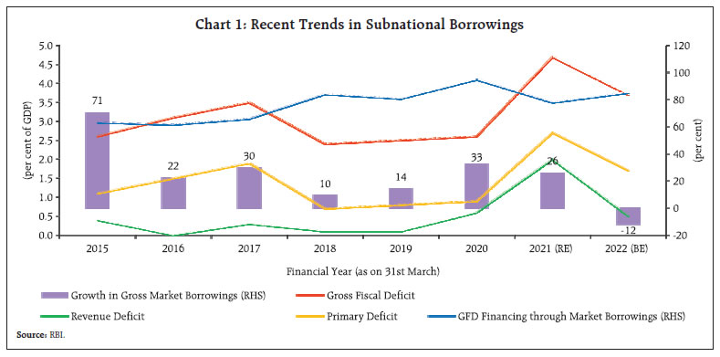 SGS yields and pandemic induced policy environment The weighted average yield on SGS softened to 6.98 per cent in FY 2021-22 from 8.58 per cent in FY 2014-15 (Chart 2), while it stood at 8.32 per cent in FY 2018-19 before the onset of the pandemic. The sharp uptick in the borrowing costs at the beginning of the pandemic was alleviated by the RBI through introduction of G-SAP in 2021-22 amounting to 2.2 lakh crores with an explicit SGS component. The weighted average spread of SGS yield over the 10-year benchmark G-sec averaged around 53 basis points during 2015-2022 while it was about 47 basis points during the last two fiscals with intermittent volatility, especially during the pandemic. Further, weighted average inter-state spread which is an indicator of the relative cost of borrowing of states on average remained low at 6 bps during FY 2014-15 to FY 2021-22 but increased to 10 basis points during FY 2020-21 amid pandemic uncertainty. A low and stable inter-state spread is evidence of non-discrimination by the market amongst states. However, it may also exhibit reluctance of market to enforce fiscal discipline through its pricing mechanisms. 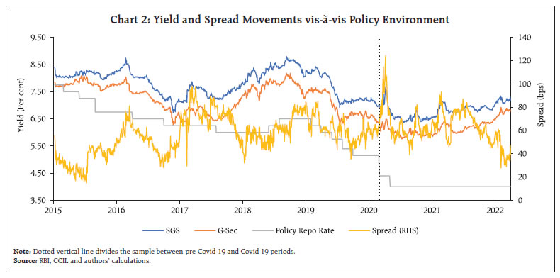 Open market operations in SGS In an unprecedented policy response to outbreak of pandemic, the RBI in October 2020 announced to conduct OMOs in SGS as a special measure to improve liquidity, facilitate efficient pricing and instil market confidence while facilitating monetary policy transmission. These OMOs were completed for a basket of SGS in three tranches amounting ₹10,000 crore each aggregating to ₹30,000 crore (Annex II). The purchases of SGS varied among states with Maharashtra scoring the highest with ₹4,818 crores while it was ₹25 crores for Goa (Chart 3). RBI followed the OMOs of SGS through a multi-security auction using the multiple price method. The allocation criteria for the SGS OMOs conducted by the RBI were mostly aligned with outstanding stock of SGS to ensure equality among the subnational issuers and was comparable with the global practices. SGS OMOs were primarily confined to the residual maturity of eight, nine and ten-year securities targeting longer end yields of SGS as per international practice with the objective of stimulating growth. As a result of this timely intervention, the SGS yields stabilised during the period of announcement from October to December 2020 along with benchmark G-Sec yields (Chart 4). Thus, the Indian experience of OMOs in subnational bonds was largely in line with global experiences in terms of the purpose, instruments, target maturities and bidding process.
Policy impact on trading, issuance pattern and ownership of SGS Both the volume as well as turnover of SGS has increased during the Covid-19 period, signifying enhanced liquidity especially following the inclusion of SGS in the G-SAPs and the OMOs in SGS securities (Chart 5). Monthly average trades in the Covid-19 period increased by 38.9 per cent while the average monthly turnover increased by 38.0 per cent compared to the pre-covid period. Further, the pandemic induced monetary policy environment of low interest rates enabled states to increase non-standard issuances6. These issuances as a percentage of the total rose to 59 per cent in Covid-19 period compared to 27 per cent during pre-Covid 19 period. Further, the average residual maturity of non-standard issuances has increased by around one year to 12.6, highlighting that states have issued non-standard securities with maturities more than 10 years during Covid-19 period to capitalise on the low cost long-term borrowing conditions (Table 1). The ownership pattern of SGS has also changed since the start of the pandemic. Chasing higher yields, corporates, financial institutions and provident funds, increased their ownership in SGS securities during Covid-19. In contrast, ownership of commercial banks and insurance companies has declined. These changes indicate the policy environment induced diversification of ownership pattern of SGS (Chart 6). | Table 1: Standard and Non-standard Primary Issuances across periods7 | | Type | Regime | Number of securities auctioned | Average Residual maturity | | Non-Standard | Covid-19 | 735 | 12.6 | | | Pre-Covid-19 | 447 | 11.5 | | Standard | Covid-19 | 544 | 10 | | | Pre-Covid-19 | 1469 | 10 | | Source: RBI and authors’ calculations. |
Pandemic and RBI facilitated cash flow management of States RBI provided enhanced cash accommodations to the states to cushion the impact of the pandemic via Ways and Means Advances (WMA) (increased by 60 per cent cumulatively, Overdraft (OD) (increased from 14 working days to 21 working days continuously and the total days of accommodation was increased from 36 working days to 50 working days in a quarter) and Special Drawing Facility (SDF). The enhanced limits remained available till March 31, 20228. Further, the scheme for constitution and administration of consolidated sinking fund (CSF)’ was also reviewed and the rules governing withdrawal from CSF were relaxed, while ensuring that a sizeable corpus is retained in the Fund (RBI, 2021). The enhanced cash accommodation facilities were utilised by the states in managing their cashflow mismatch during the pandemic period (Chart 7). 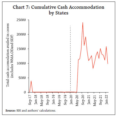 Poor cash management practices increase the effective costs of borrowings, add risks and complicate other financial policies (Williams, 2009). States can park their excess cash into intermediate treasury bills (ITBs) or auction treasury bills (ATBs) for which they earn interest that is lower than the interest outgo on market borrowings. This gives rise to negative carry - the difference between the SGS yields and returns on ITBs and ATBs investments. The crisis induced monetary policy scenario widened the negative carry of returns for the states (Chart 8). This warrants better fiscal marksmanship by states as pre-emptive over-borrowing has its associated negative carrying costs. Upgrading cash flow forecasts, recalibrating cash buffer levels and drawdown on reserve funds are some of the best cash management practices under fiscal stress (IMF, 2020). III. Empirical analysis on volatilities in yield and determinants of spread of SGS Volatility dynamics in SGS yield Apart from credit risk, bond price or yield is impacted by changes in interest rate, inflation expectation in the form of inflation risk and risk premia including maturity and liquidity risk. Further, during the periods of heightened uncertainty, yields can become highly volatile [(Azis, et al (2013), Amisano and Tristani (2019)]. The outbreak of pandemic triggered macroeconomic uncertainty and financial market volatility world-wide. Indian financial market also witnessed episodes of volatility during the period. This section attempts to analyse the volatility of SGS yield and its persistence. It examines the pricing pattern of SGS and its association with benchmark G-sec yields using Engle-Granger and Phillips- Oulliaris cointegration methodology. Further, the volatility of yields and its persistence were examined using the standard GARCH model. For the analysis, daily data on secondary market yields on benchmark 10-year G-Sec and SGS was obtained from CEIC and CCIL9, respectively for the period Jan 2015 - March 2022. | Table 2: Descriptive Statistics for SGS and G-sec Yield | | | SGS | G-Secs | | Mean | 7.50 | 7.08 | | Standard Deviation | 0.67 | 0.65 | | Skewness | -0.12 | -0.12 | | Excess Kurtosis | -1.30 | -1.28 | | Note: Values pertain to 10-year securities and belong to the period from Jan 2015 to March 2022. | A sub-national debt instrument is priced relative to a sovereign instrument plus a spread. The average SGS yield is found to be higher than G-sec yield over the period indicating the presence of a spread. The standard deviation of SGS and G-Sec yield, however, is found to be similar (Table 2). The test proposed by Levene (1960) is used to test for the null of equal variances10. The test failed to reject the null hypothesis with a p-value of 0.14 indicating that the level of volatility is similar in both series underscoring the close association of SGS with G-Sec yield. Further, cointegration tests are conducted to identify the long-term relationship between SGS and G-Sec secondary market yields and it is found that both yields are cointegrated (Table 3). The results indicate that a common underlying trend drives both yields. | Table 3: Unit Roots and Cointegration | | | Unit root tests
(H0: Presence of Unit root) | Cointegration tests
(H0: No Cointegration) | | ADF test | Phillips- Perron test | Engle-Granger test | Phillips Oulliaris test | | SGS | -1.70 | -1.98 | | | | | (0.75) | (0.61) | -4.32* | -8.34** | | G-Sec | -1.65 | -1.77 | (0.011) | (0.000) | | | (0.77) | (0.72) | | | ‘*’: Significant at 5% level, ‘**’: Significant at 1% level.
Note: Values in parenthesis are p-values. |
The rolling weekly volatility of SGS and G-Secs shows some time varying features with spikes during periods of economic stress (Chart 9). Therefore, in a scenario of volatility spikes, it is pertinent to know how quickly such shocks subside or do they persist and whether the level of persistence is same for both series. A standard GARCH model was employed to study the volatility persistence. The conditional variance of SGS and G-Secs were estimated with a standard GARCH(1,1)11 model where the mean of the process is modelled as a constant. The findings show that there is mean reversion in volatility as the estimated sum of α and β is less than one indicating that volatility shocks eventually die out in the case of SGS as well as benchmark G-sec (Table 4). Further, it shows that volatility shocks to G-Sec yield are marginally more persistent than SGS yield. Additionally, following Borio and McCauley (1996) methodology, autoregressive models of order 1 were fitted for the historical rolling weekly volatility of the two yields. The results show that the persistence parameters for SGS and G-Sec yield are significant with values, 0.910 and 0.911, respectively12, indicating similar level of persistence and confirming the results from the GARCH model. These findings imply that volatility shocks generate similar dynamics in SGS and G-sec. The marginal differences in the volatility shock persistence could be attributed to thin volumes of trades in SGS in the secondary market. The cointegration of SGS with the benchmark G-Sec and identical volatility shock dynamics highlight that any concerns on benchmark G-sec yield may also weigh on SGS yields. | Table 4: Volatility Dynamics | | Variable | G-Sec yield | Weighted-average SGS yield | | ω | 0.000** | 0.000** | | | (2.83) | (3.09) | | α | 0.100** | 0.142** | | | (3.15) | (4.69) | | β | 0.880** | 0.797** | | | (23.85) | (21.26) | ‘*’: Significant at 5% level, ‘**’: Significant at 1% level.
Note: Values in parenthesis are t-statistics. | Determinants of SGS spreads Preliminary analysis of the variation of spread13 across states indicates marginal variation across states in terms of average spread14 from January 2015 to March 2022 reflecting that the market is not differentiating much between states for pricing their debt. However, the range of spread calculated as the difference between the highest and lowest spread for a particular state over the sample period does show variation across states (Chart 10a). The average cumulative spread during the period 2015-2022 is found to be 62 basis points. However, the average spread ranged between 39 and 77 basis points while the maximum variability was witnessed in calendar year 2020 highlighting volatile financial conditions driven by pandemic induced economic uncertainty (Chart 10b). In general, other than state specific factors, various macroeconomic factors also affect the spread of sub-national debt securities. The study uncovers the determinants of SGS yield spreads across states in India through a panel data framework. Unlike previous studies on SGS spreads, this study utilises monthly data for the period from January 2015 to March 2022 to capture market dynamics in a higher frequency data framework. The study follows the panel data methodology15 using an unbalanced panel of 26 States. Taking cues from the literature on determinants of spread (YS) of SGS over the benchmark G-sec (Bose et al. (2011) and Saggar et al. (2017)), the study identifies the state specific variables such as the number of times a state participates in SGS auctions (NT) in a month and average borrowing size (SIZE) in the auctions which adds to the supply of bonds and hence expected to drive spreads upwards. Higher economic growth can lead to greater tax revenues and hence may reduce the cost of borrowing. The Index of Industrial Production (IIP) is used as a proxy for economic growth. The cash position of the states (INVS) is proxied by their investments in intermediate treasury bills (ITBs) while the market factors are captured through liquidity conditions (LAF) and short-term rate expectations (OIS1Y). Secondary market trading volumes can affect the illiquidity premium charged on a state’s borrowings and to capture this effect, average trading size in a month (TRAD) is used while a crisis dummy variable (CRISIS) is added to control for any systemic impact caused by the pandemic (Table 5). 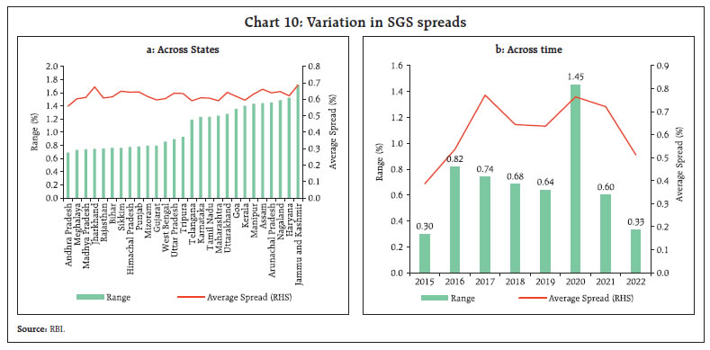 The panel unit root test for checking stationarity of variables is conducted using the Covariate Augmented Dickey-Fuller (CADF) test by Hansen (1995) as extended by Constantini and Lupi (2011) to account for the cross-sectional dependence in panel data, which finds no evidence of unit roots16. The estimates of the panel data models and the Hausman test17 and F-test18 conducted shows fixed effects model is an appropriate choice over other models. Residual diagnostics for fixed effects model indicate presence of heteroskedasticity, serial correlation and cross-sectional dependence (Table 6). The selected fixed effects model is thus corrected using Driscoll-Kraay standard errors (Table 7).19 | Table 5: Data description for the panel data model | | Variable name | Description | | YS | Yield spread over G-Secs for SGS | | NT | No. of auctions participated in by each state in the month | | SIZE | Logarithm of monthly average size of auction for each state | | IIP | IIP growth rate year-on-year | | INVS | State government cash surplus investments in ITBs | | LAF | Dummy variable signifying liquidity conditions, 1 for net LAF injection and 0 for net LAF absorption | | OIS1Y | Rate on 1-year OIS contract | | CRISIS | Dummy variable to capture the impact of pandemic | | TRAD | Average trade size of a particular state’s SGS in a month in secondary market | | Source: RBI, Bloomberg and CEIC | The results highlight that the outbreak of the pandemic did impact the spread of SGS as seen from the positive and significant coefficient on CRISIS dummy variable. Further, the average auction size for a state is found to be significant with positive sign indicating that increased borrowings result in higher costs underscoring the supply concerns of the market. Also, cross-sectionally invariant variables signifying the economic growth scenario (IIP) and liquidity conditions (LAF_dum) are found to be significant implying that the existing macroeconomic and financial conditions weigh on the SGS spreads. Interestingly, significant cash surpluses by states in terms of investments in ITBs (INVS) tend to result in higher spread reflecting that a premium is charged for poor fiscal marksmanship in cash management. As large cash surpluses have accompanying negative carry cost costs, therefore, states should try to limit pre-emptive over borrowings which can also ease supply concerns of the market. | Table 6: Residual Diagnostic Tests | | | Breusch-Pagan Test
H0: Homoskedasticity | Breusch-Godfrey/ Woolridge test for serial correlation
H0: No serial correlation | Breusch-Pagan LM test
H0: No cross sectional dependence | | Test Statistic | 370.68***
(0.000) | 37.383***
(0.005) | 5487.4***
(0.000) | | Inference | Heteroskedasticity | Serial autocorrelation. | Cross-sectional dependence | Note: Values in parenthesis are p-values.
*** : 1% significance, ** : 5% significance, * : 10% significance. |
| Table 7: Panel Data Estimations | | Variables | Dependent Variable: YS | | Pooled OLS | Fixed Effects | Random Effects | Fixed Effects model corrected by D-K Standard Errors | | NT | 0.002
(0.007) | 0.010
(0.007) | 0.002
(0.007) | 0.010
(0.008) | | SIZE | 0.008
(0.006) | 0.063***
(0.013) | 0.009
(0.006) | 0.063***
(0.020) | | IIP | -0.289***
(0.042) | -0.302***
(0.041) | -0.289***
(0.042) | -0.302*
(0.180) | | INVS | -0.001
(0.001) | 0.002**
(0.001) | -0.001
(0.001) | 0.002**
(0.001) | | LAF_dum | -0.133***
(0.016) | -0.119***
(0.016) | -0.132***
(0.016) | -0.119**
(0.047) | | OIS1Y | -0.016**
(0.007) | -0.014**
(0.007) | -0.016**
(0.007) | -0.014
(0.021) | | TRAD | -0.009
(0.018) | -0.023
(0.019) | -0.009
(0.018) | -0.023
(0.021) | | Crisis | 0.108***
(0.021) | 0.111***
(0.021) | 0.108***
(0.021) | 0.111*
(0.061) | | Constant | 0.681***
(0.055) | | 0.678***
(0.056) | | | Observations | 1,232 | 1,232 | 1,232 | 1,232 | | Adjusted R2 | 0.226 | 0.229 | 0.226 | 0.229 | Note: Values in parenthesis are standard errors.
*** : 1% significance, ** : 5% significance, * : 10% significance. | IV. Conclusion The global practices in the asset purchase programme of subnational securities suggests that subnational assets/securities have the potential to become supplementary tool in the monetary policy toolkit of central banks. The Reserve Bank’s decision to include SGS in G-SAP was well calibrated and was broadly in line with the global practices. The measures taken by the RBI with conducive monetary and financial conditions facilitated the higher market borrowings of states to cope with pandemic induced economic uncertainty. The empirical findings of cointegration of SGS with the benchmark G-Sec and identical volatility shock dynamics highlight that any concerns on benchmark G-sec yield may eventually weigh on SGS yields. Further, panel data analysis reveals that increase in borrowings results in a higher spread of SGS underscoring the supply concerns of the market. The findings also highlight that pre-emptive over-borrowing resulting in larger investments in ITBs has its associated cost in terms of higher cost of borrowing as well as significant negative carry costs. This reflects the need for improved fiscal marksmanship by states. Following efficient cash management practices can reduce pre-emptive over-borrowing and the effective cost of borrowings while easing the supply concerns of the market. References Allen, R., Balibek, E., Hurcan, Y. and Saxena, S (2020), “Government Cash Management Under Fiscal Stress.” FAD Note, International Monetary Fund. Amisano, Gianni and Tristani, Oreste, Uncertainty Shocks, Monetary Policy and Long-Term Interest Rates (May 10, 2019). ECB Working Paper No. 2279 (2019); ISBN 978-92-899-3541-8, Available at SSRN: https://ssrn.com/abstract=3387270 or http://dx.doi.org/10.2139/ssrn.3387270. Azis, I.J., S. Mitra, A. Baluga, and R. Dime. 2013. The Threat of Financial Contagion to Emerging Asia’s Local Bond Markets: Spillovers from Global Crises. ADB Working Paper Series on Regional Economic Integration No. 106. January. Borio, C., & McCauley, R. N. (1996). “The economics of recent bond yield volatility”. BIS Economic Papers Bose, D., Jain, R., & Lakshmanan, L. (2011). “Determinants of Primary Yield Spreads of States in India: An Econometric Analysis.” RBI Working Paper Series, WP 10/2011. Constantini, M. & Lupi, C. (2013) A simple panel-CADF test for unit roots. Oxford Bulletin of Economics and Statistics, 75, 276–296. Hansen, B. E. (1995). “Rethinking the univariate approach to unit root testing: using covariates to increase power”. Econometric Theory, Vol. 11, pp. 1148–1171. Hoechle, D. (2007). Robust Standard Errors for Panel Regressions with Cross-Sectional Dependence. The Stata Journal, 7(3), 281-312. https://doi.org/10.1177/1536867X0700700301. Jose, J., Mishra, P. and Pathak, R. (2021), “Fiscal and monetary response to the COVID-19 pandemic in India”, Journal of Public Budgeting, Accounting & Financial Management, Vol. 33 No. 1, pp. 56-68. https://doi.org/10.1108/JPBAFM-07-2020-0119 H. Levene, “Robust Tests for Equality of Variances,” In: I. Olkin, et al., Eds., Contributions to Probability and Statistics: Essays in Honor of Harold Hotelling, Stanford University Press, Palo Alto, 1960, pp. 278-292. RBI, “Chapter VII: Public Debt Management”, Annual Report, 2022. Saggar, S., Rahul, T. & Adki, M. (2017). “State government yield spreads – Do fiscal metrics matter?” RBI Mint Street Memo, No. 08/2017, Reserve Bank of India. Williams, M. (2009). “Government cash management: international practice.” Oxford Policy Management Working Paper 2009-01.
| Annex I: Subnational bond purchase programmes of select countries | | Country/ Jurisdiction | Programme/Objective | Eligible Instruments/ Mode of Purchase | Allocation Criteria | Additional Criteria | | Euro Area | | -
Euro-denominated marketable debt instruments viz., nominal and inflation- linked central government bonds, bonds issued by recognised agencies, regional and local governments, international organisations and multilateral development banks located in the euro area -
Direct purchase and reverse auction in secondary market. | Capital Key- according to the capital share of each member countries in ECB. | | | United States | | -
Tax anticipation notes (TANs), tax and revenue anticipation notes (TRANs), bond anticipation notes (BANs), revenue anticipation notes (RANs), and other similar short-term notes issued by eligible issuers. -
The SPV created purchases eligible notes directly from eligible issuers at the time of issuance (Primary market). | Population thresholds/ at least two cities or counties eligible | -
Maturity not later than 36 months from the date of issuance. -
Credit Rating. -
Up to an aggregate amount of 20% of general revenue from own sources and utility revenue of applicable State, City, or County.
Up to an aggregate amount of 20% of gross revenue of the Multi-State Entity or Designated revenue bond issuers, as reported in its audited financial statements. | | Sweden | -
Municipal bond purchases for monetary policy purposes -
To keep general interest rates low, facilitate credit supply and to safeguard the monetary policy transmission | | Equal treatment of issuers in terms of maturity and credit rating. | Credit rating | | Canada | Provincial Money Market Purchase Program (PMMP) Provincial Bond Purchase Program (PBPP)
Support the liquidity and efficiency of provincial government funding markets | | Share of the issuer’s debt outstanding as well as the issuer’s share of Canada’s GDP | -
PMMP -40 per cent (initially) of each offering of directly issued provincial money market securities with terms to maturity of 12 months or less -
PBPP -No purchases more than 20% of an issuer’s eligible assets outstanding. -
No minimum rating requirement | | Australia | | | Allocation between semis is guided by the stock of debt outstanding and relative market pricing. | | | New Zealand | | -
LSAP programme includes NZ Government Bonds, Local Government Funding Agency Bonds and NZ Government Inflation-Indexed Bonds. -
Secondary market purchase through auctions from eligible counter parties. | 30 per cent of the total debt issuances of LGFA | 1 to 13 years maturity as governed by LGFA bonds on issue | Source: Respective Central Banks web releases. |
| Annex II: OMO Purchases of SGS by RBI | | (Amount in ₹ Crore) | | Sl. No | State | OMO-I | OMO-II | OMO-III | Total Purchase | Total Purchase | | Offered | Accepted | Yield (%) | Offered | Accepted | Yield (%) | Offered | Accepted | Yield (%) | Accepted OMO | as % of total OMO | | 1 | Andhra Pradesh | 65 | 65 | 6.50 | | | | | | | 65 | 0.22 | | 2 | Arunachal Pradesh | 585 | 585 | 6.56 | | | | | | | 585 | 1.95 | | 3 | Assam | 700 | 570 | 6.57 | | | | | | | 570 | 1.90 | | 4 | Bihar | 444 | 230 | 6.53 | | | | 1021 | 750 | 6.51 | 980 | 3.27 | | 5 | Chhattisgarh | 200 | 100 | 6.55 | | | | | | | 100 | 0.33 | | 6 | Goa | 25 | 25 | 6.65 | | | | | | | 25 | 0.08 | | 7 | Gujarat | 1287 | 1060 | 6.52 | | | | 2368 | 1498 | 6.48 | 2558 | 8.53 | | 8 | Haryana | 2279 | 1449 | 6.53 | | | | 65 | 65 | 6.52 | 1514 | 5.05 | | 9 | Himachal Pradesh | 428 | 315 | 6.57 | | | | | | | 315 | 1.05 | | 10 | Jammu and Kashmir | 145 | 135 | 6.57 | | | | | | | 135 | 0.45 | | 11 | Jharkhand | 136 | 135 | 6.60 | | | | | | | 135 | 0.45 | | 12 | Karnataka | 4265 | 2335 | 6.49 | | | | 1369 | 1279 | 6.43 | 3614 | 12.05 | | 13 | Kerala | 255 | 55 | 6.55 | | | | | | | 55 | 0.18 | | 14 | Madhya Pradesh | 1127 | 647 | 6.52 | | | | | | | 647 | 2.16 | | 15 | Maharashtra | 3534 | 2294 | 6.50 | | | | 2821 | 2524 | 6.51 | 4818 | 16.06 | | 16 | Manipur | | | | 184 | 184 | 6.44 | | | | 184 | 0.61 | | 17 | Meghalaya | | | | 372 | 370 | 6.44 | | | | 370 | 1.23 | | 18 | Mizoram | | | | 433 | 221 | 6.44 | | | | 221 | 0.74 | | 19 | Nagaland | | | | 233 | 233 | 6.45 | | | | 233 | 0.78 | | 20 | Odisha | | | | 175 | 110 | 6.43 | | | | 110 | 0.37 | | 21 | Puducherry | | | | 49 | 3 | 6.36 | | | | 3 | 0.01 | | 22 | Punjab | | | | 785 | 405 | 6.41 | 745 | 730 | 6.57 | 1135 | 3.78 | | 23 | Rajasthan | | | | 2181 | 1306 | 6.39 | 1854 | 1109 | 6.52 | 2415 | 8.05 | | 24 | Sikkim | | | | 380 | 290 | 6.43 | | | | 290 | 0.97 | | 25 | Tamil Nadu | | | | 2916 | 2625 | 6.36 | 667 | 667 | 6.47 | 3292 | 10.97 | | 26 | Telangana | | | | 363 | 363 | 6.44 | | | | 363 | 1.21 | | 27 | Tripura | | | | 128 | 121 | 6.55 | | | | 121 | 0.40 | | 28 | Uttarakhand | | | | 79 | 52 | 6.43 | | | | 52 | 0.17 | | 29 | Uttar Pradesh | | | | 3411 | 2396 | 6.42 | 577 | 422 | 6.51 | 2818 | 9.39 | | 30 | West Bengal | | | | 1331 | 1321 | 6.41 | 1086 | 956 | 6.53 | 2277 | 7.59 | | | Total /Avg Yield | 15475 | 10000 | 6.55 | 13020 | 10000 | 6.43 | 12573 | 10000 | 6.51 | 30000 | 100 | Note: Yield is calculated as the weighted average cut-off yield weighted by the amount accepted for each security in the auction.
Source: RBI |
^ The authors are from the Department of Economic and Policy Research. * The views expressed in this article are those of the authors and do not represent the views of the Reserve Bank of India. 1 The nomenclature of the State Development Loan (SDL) has been changed to State Government Security (SGS) from July 2022 onwards. 2 As per available budgetary and provisional estimates from National Statistical Office (NSO). 3 The data from January 2015 till March 2022 is used in this section for comparison. Pre-COVID-19 period wherever mentioned pertains to the period from January 2015 to February 2020 and COVID-19 period pertains to the period from March 2020 to March 2022. 4 As per RBI’s Annual Reports 2015 to 2022. 5 As per RBI’s State Finances : A Study of Budgets various issues. 6 Standard issuances refer to securities with 10-year maturity while non-standard issuances refer to securities with maturity other than 10 years. 7 Pre-Covid period: January 2015 – February 2020. Covid-19 period: March 2020 – March 2022. 8 As per RBI’s press release dated 01-04-2022 : https://www.rbi.org.in/Scripts/BS_PressReleaseDisplay.aspx?prid=53499 9 CCIL SDL Index provides daily yields of 14 most recently issued 10-year maturity securities of 14 States. 10 Levene’s test controls for non-normality of underlying distributions and both yields strongly reject the null of normality in D’Agostino and Pearson’s test. 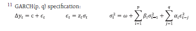
12 Standard errors were corrected using Newey-West methodology. 13 The difference between 10-year SGS yield and 10-year benchmark G-Sec yield. 14 This is calculated as the average spread across the entire period for a particular state. 15 All models and tests are run using ‘plm’ package in R. 16 CADF test statistic: -23.92*** (0.000). *** at 1% significance. Values in parenthesis are p-values. H0: All the series are I(1). 17 Hausman Test statistic: 18.45***(0.018); ***: 1% significance. Values in parenthesis are p-values; H0: Random effects model is preferred. 18 F-test for individual effects: 2.13*** (0.001); ***: 1% significance. Values in parenthesis are p-values; H0: No individual effects or Pooled OLS model suffices. 19 Erroneously ignoring cross-sectional correlation in the estimation of panel models can lead to severely biased statistical results. Hoechle (2007) uses Monte Carlo simulations to analyse statistical properties of various variance-covariance estimators vis-à-vis Driscoll-Kraay (DK) estimators which controls for cross-sectional dependence along with heteroskedasticity and serial correlation and found that DK standard errors are well calibrated when cross-sectional dependence is present. |