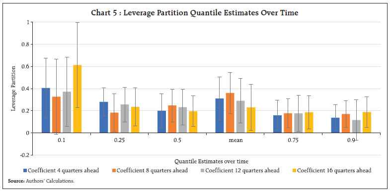
by Saurabh Ghosh^{^}, Vidya Kamate^{^} and Ria Sonpatki^#

This article analyses the role of domestic and international macro-financial conditions in influencing the future distribution of GDP growth for India using a Growth-at-Risk (GaR) framework. The GaR framework, by assessing the entire distribution of future GDP growth, helps in quantifying the likelihood of tail risk scenarios i.e. lower quantiles of GDP growth. GaR framework projections are not baseline forecasts of growth but shed light on low probability extreme events and are in the nature of stress tests that serve as a useful tool for monitoring risks to financial stability and macro-prudential policy implementation.

Introduction

Sustained and inclusive economic growth can lead to progress, creation of decent jobs for all, and improved per capita income levels. Therefore, it is unsurprising that growth rate of Gross Domestic Product (GDP) of an economy has increasingly become an important parameter to gauge a nation’s economic well-being and its relative economic performance vis-à-vis the rest of the world. Globally, numerous inflation targeting central banks, routinely publish their forecasts of GDP growth rate in addition to the inflation rate. They usually provide point estimates for the conditional mean of economic variables or fan charts. However, with growing economic uncertainty and shocks, e.g. COVID-19 pandemic and Russia-Ukraine War etc., it has become increasingly important to understand the entire distribution of target economic variables and minimise the downside risks. The Growth-at-Risk (GaR) concept addresses the questions relating to the worse outcome with certain probability. It was informally introduced in the April 2017 edition of Global Financial Stability Report (IMF 2017a) and its analytical underpinnings were provided in October 2017 (IMF 2017b). Both reports analysed how prevailing global financial conditions may affect tail risks to global economic activity. The GaR framework developed by Adrian et al. (2019) and the practical guidance on its implementation by Prasad et al. (2019). The Bank of England also computes GaR for its policy analysis¹. Patra et al. (2022) draws on recent developments in the ‘capital flows at risk’ framework for India using a similar framework. In this backdrop, the article applies the GaR framework to India to understand and quantify the different dimensions of macro-financial risks to future GDP growth.

The opening up of Indian economy since 1991, bilateral trade with other countries, combined with financing from external markets made it vulnerable to global macroeconomic shocks such as the Global Financial Crisis of 2007-08. In a highly interconnected and increasingly synchronised global economy, not just domestic financial developments but international risk spillovers can generate downside risks to domestic economic growth (Ghosh et al., 2017; Kamate and Ghosh, 2022). The macroeconomic aftermath of global financial crisis was a vivid reminder of the significant consequences and highlight the need for early warnings that must be sent, and actions that must be taken to mitigate the associated tail risks (Aikman, 2019). In fact, policymakers in recent years have increased their focus on downside risks, especially in wake of recent global shocks such as the COVID-19 pandemic and Ukraine-Russia War. Most inflation-targeting central banks release GDP and inflation distributions in addition to mean forecasts.

In this backdrop, this article attempts to apply the GaR framework to assess the tail risks to growth for India. The rest of the article is organised as follows. Section II provides a brief overview of the literature analysing tail risk estimation and some recent applications of GaR framework to other economies. Section III provides a detailed overview of the data and methodology used in the GaR analysis for India. Section IV highlights the main empirical results, and Section V concludes.

II. Review of Literature

The concept of “tail risk” is a critical factor in modern risk management and financial regulation. Tail-based risk indicators have become the standard metrics for measuring risk, and their use is widespread in banking and insurance regulatory frameworks such as Basel III (BCBS 2016). Such risk measurements investigate the “tail” or “shortfall” of a risk at or below a given threshold. While most tail risk events relate to some aggregate macroeconomic shocks, tail real risks might also emanate from an interplay between microeconomic shocks and sectoral heterogeneity (Acemoglu et al., 2017). While the entire distribution of GDP growth evolves over time, the left tail of the distribution was found to be positively correlated with slack in financial conditions (Adrian, et al. 2019). The conventional estimation of tail risk was based on Value-at-Risk (VaR) approaches, but these models underperformed in the face of extreme price movements which led to the emergence of expected shortfall measure (Artzner et al., 1999). The conditional distribution of GDP growth as a function of financial conditions and macroeconomic vulnerabilities was first modelled in Adrian et al. (2019). It was found that the lower quantiles of GDP growth tended to vary with financial conditions, while the upper quantiles were more stable over time.

The practical guidance on GaR analysis that is implemented in the current article uses GaR tools that were subsequently developed by Prasad et al. (2019). Accordingly, this toolkit helps to estimate projections for both financial and macroprudential surveillance through presenting early indicators of potential problems. The GaR approach has been used to investigate growth distributions in various economies. Examples show that changes in macroeconomic conditions affect growth differently in various nations, and that changes over time are nonlinear. For instance, in Albania (IMF 2019a), economic circumstances in trade partners have the greatest short-run impact on growth; but, in Portugal, domestic financial conditions (including interest rates, leverage, and credit expansion) tend to be more important drivers of future GDP growth (IMF 2018b). Similarly, external financial circumstances, such as interest rates or currency rates, have the most explanatory power for Singapore’s future GDP growth (IMF 2018a). Recently, one such analysis for India suggests that a negative credit shock increases downside risk to growth (MacDonald and Xu, 2022). Considering the heterogeneity of shocks on growth rate distribution, this article contributes to this growing strand of empirical literature, by applying this framework for an important emerging market economy, India.

III. Data and Methodology

Using the financial market idea of Value-at-Risk as an inspiration, Growth at risk (GaR) strives to comprehend the worst-case scenario of GDP at a certain probability level i.e. the probability of future real GDP growth falling below a pre-specified threshold. Formally, GaR is defined using the equation below.

where y_t denotes the real GDP growth rate, GaR^y_t is implicitly defined as the threshold below which real GDP growth occurs with probability α conditional on the information set available at time t. GaR model is computed by firstly, categorising the financial and macroeconomic variables into relevant partitions. The partitions are then converted to indices using Principal Component Analysis (PCA) which helps to reduce parameter dimensionality and idiosyncratic noise. To comprehend the non-linear relationships between the chosen variables and GDP growth, quantile regression is estimated at 10th, 25th, 50th, 75th and 90th quantiles. This produces a baseline estimate of the entire GDP growth distribution. A skewed-t-distribution is then fitted, which contains four parameters – mean, variance, skewness, and shape. The GaR for a given threshold probability value is obtained by using this distribution. To understand forecasts of GaR over short, medium, and long-term, multiple horizon projections are estimated ranging from 4 to 16 quarters ahead, giving an insight on the differential temporal effects of the various variable partition groups. A stress testing exercise is also conducted to understand how shocks to individual or multiple partitions can cause deviation in the distribution of future GDP growth from baseline outlook. Quarterly data from 2001 Q3 to 2022 Q1 for GDP is obtained from CEIC, financial market data is obtained from Bloomberg, and credit related variables are obtained from the Reserve Bank’s DBIE². Variables influencing GDP growth from domestic as well as global sectors are considered. For some of the credit related variables whose data is released with a lag, we use their forecasted value³ for the analysis.

Domestic variables such as credit and financial conditions have a direct beneficial impact on GDP growth and tend to provide information on risks to growth. Through effective and efficient capital mobilisation and allocation, credit market expansion has the potential to stimulate riskier investments in profitable channels (Mishra et al., 2009). Additionally, the financial conditions index serves as a useful tool for predicting GDP growth especially in the short run at lower quantiles (Prasad et al., 2019). Domestic financial conditions represent the domestic price of risk, cost of domestic borrowing for individuals and corporations and in general, costs of financing investment projects in the local economy. The combination of financial market and credit cycle indicators provides information on the evolution of financial sector stress and financial stability threats. Thus, evaluating financial vulnerabilities yields considerable information on future growth concerns (Acharya et al., 2020). Lastly, in addition to domestic financial conditions, the crucial role of foreign vulnerabilities in determining downside risk to domestic growth is well documented (Lloyd et al., 2021). Foreign financial developments can influence domestic growth through multiple channels, e.g. cross-country co-movement of asset prices, influencing costs of foreign claims of domestic financial institutions and macro-economic channels such as demand for domestic exports. Keeping these factors in mind, variables suitable for explaining the dynamics of GDP growth were selected. These variables were divided into three broad groups that capture domestic financial conditions, leverage conditions and global conditions respectively (Table 1). Principal Component Analysis (PCA) was conducted on grouped variables to extract common trends from the large array of indicators⁴. Domestic Financial Conditions partition captures the domestic price of risk that comprises interbank spreads, term premiums, bond returns, bond returns volatility, equity returns, and equity returns volatility, and long-term costs of funding. Similarly, Leverage partition captures information on credit aggregates and banking sector stress. Finally, global conditions partition captures global supply chain disruptions, financial market stress and currency movements.

IV. Empirical Results

The first crucial step in GaR analysis is selecting relevant variables and assembling partitions. Instead of considering variables individually, partitions are built based on their proclivity to co-move with one another, since they represent comparable underlying factors and aid in the extraction of common patterns. As mentioned in the previous section, PCA is done on the three selected partitions to turn a set of observations of potentially correlated variables into a set of values of linearly uncorrelated variables that will be utilised to conduct quantile regression.

a) Factors that Matter: Principal Component Analysis

The first principal component for each partition is considered. PCA loadings that accompany each partition give information on the relative significance of variables examined under each partition. Along the Domestic Financial Conditions Partition, Interbank Spread, 10-year and 5-year Corporate Bond Spread are the most influential drivers of domestic financial conditions as they explain almost 50 per cent of variation within the partition (Chart 1). A higher value of this partition implies a tightening of domestic financial conditions.

Leverage partition captures overall credit conditions in the economy. The significant contributors to this partition are credit-to-GDP ratio, credit-to-deposit ratio and non-resident liabilities that explain approximately 87 per cent variation in the partition (Chart 2).

Among the variables comprising Global Conditions partition, the Baltic Dry Index is the most significant, followed by US equity market volatility, oil price and REER for India.

b) Asymmetric Tail Risks: Quantile Analysis

Variables do not necessarily behave the same way at the extremes of the distribution as they do at the centre, where the entire distribution varies over time and not just the central tendency. Quantile regression aids in estimating the non-linear connection and identifying the components that are crucial distribution drivers. For acknowledging non-linear relationship between financial conditions, macro-financial vulnerabilities quantile regressions are estimated at 10th, 25th, 50th, 75th and 90th quantiles of future GDP growth and independent variables (3 partitions).

The quantile regression takes the following form:

Domestic Financial Conditions are an excellent predictor of downside risks to India’s GDP growth over shorter horizon of 4 quarters. The projected impact of increased risk pricing appears to be strongest towards the tails of the GDP growth distribution rather than around the mean, confirming the assumption of asymmetries in the output response (Chart 3).

A tightening of financial conditions provides a considerable negative risk to growth at the lower quantiles (Chart 3). For brevity we haven’t reported financial circumstances over the next eight to sixteen quarters, as our empirical findings indicate that they become uninformative signifying that financial conditions could only provide meaningful information for GDP growth in the short future.

Quantile regression coefficients of Global conditions partition highlight the differentiated effects of global shocks on future GDP growth (Chart 4). For instance, a significant negative impact of Global conditions is observed at lower quantiles (10th) as well as at upper quantiles (75th). This result is consistent with the literature for quantile regression. It may be noted that mean estimates are not significant, though upper and lower quantiles are. Therefore, this highlights that crucial information would be lost if this non-linearity is not appropriately uncovered via quantile regressions. It is observed that Global conditions while representing a downside risk to growth in the near term, pose an upside risk for 8 quarters ahead horizon. Leverage partition signals upside risks to GDP growth at horizons 4 to 16 quarters ahead (Chart 5). Given that India is an emerging market economy, growing credit aggregates, beyond a threshold (RCF 2022), indicate more upside risks to growth.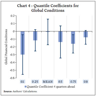

c) Estimating GaR

A skewed-t-distribution is then fitted by interpolating between the estimated quantiles to smooth the quantile function and translate the empirical quantile distribution into an estimated conditional distribution of GDP growth (Patra et al., 2022). The skewed-t-distribution is fully described by four parameters (location, degree of freedom, scale, and skewness) and is therefore a concise yet comprehensive approach to synthesize variance (volatility), kurtosis and skewness. In comparison to the t-distribution, the skewed-t-distribution has a shape parameter that controls how much skewing influence it has on its probability distribution function.

The fitted skewed distribution allows the estimate of GaR that signifies the probability of future growth rate falling under an estimated GDP growth value (Chart 6.a). The density highlighted at 10 per cent can be utilised to construct a measure of risk to GDP growth associated with prevailing financial and macro-economic conditions. GaR at 10 per cent denotes that there is a 10 per cent probability that GDP growth 4 quarters ahead could be less than or equal to the threshold value. The conditional forecasts of GDP growth, based on the financial conditions and selected macro-financial vulnerabilities, are used by GaR model to quantify the impact of realisation of risk. Given that our dataset includes observations pertaining to the pandemic period, which was indeed a black swan event, academic interest prompted us to drop the pandemic time observations and re-compute GaR (Chart 6.b) to check how much would the Growth-at-risk numbers change for India by exclusion of this event. In line with our expectation, the entire distribution shifts to the right, indicating improvements in GaR at 10 per cent level and in the measures of central tendencies.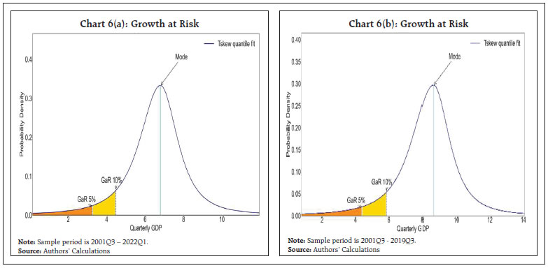

d) Multiple Horizon Projections and Stress Tests

The longer is the left tail of the distribution, the higher are the tail risks to the growth, which serves as an early warning indicator. To assess GaR at medium and longer term, future horizon projections are analysed. Accordingly, distributions of GDP growth are projected for 4,8,12,16 quarters ahead to give an understanding of the future growth of India (Chart 7). The 4 quarters ahead forecast scenario appears challenging especially during recovery phase of Covid-19, Russia-Ukraine crisis and a slowdown in World GDP growth. Deteriorations in domestic and global financial conditions coincide with declines in the mean and increases in the variance of the future GDP growth distribution, thus with the leftward shift of the distribution. When vulnerabilities develop, the likelihood of a more catastrophic situation increases and hence, a leftward shift indicates higher tail risks to growth.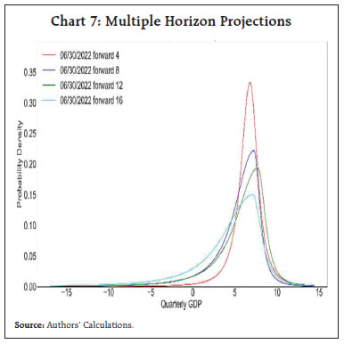

Comparing the conditional density across the quarters, significant time variation in the density is observed, and this time variation is primarily due to the changes in the lower tail of the distribution.

The GaR model is used to lead a stress testing exercise for generating macro-financial scenarios. Given that the present GaR architecture is a lean reduced form forecasting system, the scenario analysis is based on comparative statics, which takes uncorrelated shocks into account without accounting for endogenous feedback. With the present global uncertainties caused by growing inflation, the Russia-Ukraine crisis etc., global conditions partition is shocked to estimate how the future GDP growth distribution may alter. This gives information on how the realisation of a risk influences the growth distribution in future periods. An adverse one standard deviation shock to global conditions diminishes average future growth (Chart 8). Furthermore, the growth distribution’s shape has changed, altering the skewness, following the shock. After the shock, the distribution becomes more negatively skewed, with a longer and fatter left tail.

V. Conclusion

The accessibility of forward-looking information is vital to the success of macroeconomic policies. GaR analysis offers an alternative baseline for evaluating the gravity of catastrophic situations because it can estimate the entire distribution of future GDP growth. The GaR technique offers the additional benefit of accounting for macro-financial vulnerabilities and serves as a warning signal in response to which macroprudential policies can be appropriately tweaked. In certain circumstances, assessments of both the baseline growth forecast and vulnerability from the tail events assumes importance in shaping pre-emptive and preventive policies. GaR framework provides an appropriate toolbox for monitoring such developments.

In light of its significance, we first make an effort to draw attention to the local and global factors that do, in fact, matter in the GaR framework. In the short-term, our research emphasises that financial conditions, global conditions, and leverage assume importance. But, in the medium term, domestic credit or leverage conditions tend to be the most significant determinant of future distribution of GDP growth. This outcome is in line with other empirical studies (IMF 2018b, IMF, 2017) and the volatility paradox (Brunnermeier and Sannikov, 2014).

Secondly, this research includes analysis of financial conditions and macro-financial vulnerabilities exploiting potential non-linearities. In this connection, the relevance of using quantile regressions is illustrated by the fact that while the mean exhibits insignificance, the lower and upper quantiles of the dependent variable demonstrate the presence of potential growth risks for India. Therefore, if just measures of central tendency and not the complete range of economic outcomes were considered, this lesson could have been missed.

Further, based on selected macro-financial data, our GaR estimates highlight the significance of credit aggregates in a developing economy like India, which necessitate their close monitoring. Global financial market volatility is found to have negative impact on domestic GDP, and therefore geopolitical developments affecting GaR may require continuous vigil.

Our study lends itself to more informed policy decisions, because it explicitly links systemic risk indicators to economic outcomes. It may help stepping up supervision of financial markets in response to warning signals by increasing the rigor of stress testing or turning on pre-existing macro-prudential instruments to address systemic risk. Though current GaR forecasting system is still emerging, it shows great promise, and the GaR-related methods will remain a crucial futuristic tool for policymakers.

References

Acemoglu, D., Ozdaglar, A., and Tahbaz-Salehi, A. (2017). “Microeconomic origins of macroeconomic tail risks”. American Economic Review, 107(1), 54-108.

Acharya, V. V., Bhadury, S., and Surti, J. (2020) “Financial Vulnerability and Risks to Growth in India”. NBER Working Paper Series

Adrian, T., Boyarchenko, N., and Giannone, D. (2019). “Vulnerable growth”. American Economic Review, 109(4), 1263-89.

Aikman, D., Bridges, J., Hoke, S. H., O’Neill, C., and Raja, A. (2019). “How do financial vulnerabilities and bank resilience affect medium-term macroeconomic tail risk”. Bank of England Staff Working Paper, (824).

Artzner, P., Delbaen, F., Eber, J. M., and Heath, D. (1999). “Coherent measures of risk”. Mathematical finance, 9(3), 203-228.

BCBS, (2016) “Explanatory note on the revised minimum capital requirements for market risk”.

Brunnermeier, M. K., and Sannikov, Y. (2014). “A macroeconomic model with a financial sector”. American Economic Review, 104(2), 379-421.

IMF. (2017). – “Is Growth at Risk?” Global Financial Stability Report, October.

Ghosh, S. and Saggar, M. (2017). “Volatility Spillovers to the Emerging Financial Markets during the Taper Talk and Actual Tapering”. Applied Economics Letters. 24:2, 122-127

IMF (2008). “Financial Stress and Economic Downturns.” World Economic Outlook (October). Chapter 4.

IMF (2017a). “Are Countries Losing Control of Domestic Financial Conditions?” Global Financial Stability Report (April). Chapter 3.

IMF (2017b). “Financial Conditions and Growth at Risk.” Global Financial Stability Report (October). Chapter 3.”

IMF (2018a). Singapore “2018 Article IV Consultation- Press Release; Staff Report; And Statement by The Executive Director for Singapore”, IMF Country Report No. 18/245.

IMF (2018b). “Portugal: Selected Issues”, IMF Country Report No. 18/274, September

IMF (2019a). “Albania: Staff Report for the 2018 Article IV Consultation.” IMF Country Report No. 19/29.

Kamate, V. and Ghosh, S. (2022). “Fed Taper and Indian Financial Markets: This Time is Different”. Reserve Bank of India Bulletin, July

Lloyd, S., Manuel, E., and Panchev, K. (2021). “Foreign vulnerabilities, domestic risks: the global drivers of GDP-at-Risk”. Bank of England Working Paper

MacDonald, M., and Xu, T. (2022). “Financial Sector and Economic Growth in India”. IMF Working Paper

Mishra, P. K.; Das, K. B. and Pradhan, B. B. (2009). “Credit Market Development and Economic Growth in India”, Middle Eastern Finance and Economics, ISSN: 1450-2889, Issue 5

Patra, M.D., Behera, H. and Muduli, S. (2022). “Capital Flows at Risk: India’s Experience”. Reserve Bank of India Bulletin. June

Prasad, M. A., Elekdag, S., Jeasakul, M. P., Lafarguette, R., Alter, M. A., Feng, A. X., & Wang, C. (2019). “Growth at risk: Concept and application in IMF country surveillance”. International Monetary Fund

RBI (2022). Report on Currency and Finance (RCF) 2021-22, April.

^ The authors are Director and Manager-Research at the Strategic Research Unit (SRU), Department of Economic and Policy Research.

^# Ria Sonpatki was a Research Intern (RI) at SRU.

* The views expressed in this article are those of the authors and do not represent the views of the Reserve Bank of India.

¹ https://www.bankofengland.co.uk/working-paper/2019/credit-capital-and-crises-a-gdp-at-risk-approach

² Many of the important financial market rate variables are not available for periods prior to 2001 which constrained us to begin our sample in 2001.

³ Random walk models are used to predict one-quarter ahead forecasts.

⁴ The GaR framework performs a PCA analysis for reducing the dimensions of the data not for capturing a latent unobservable variable and, as such, assumes that all variance can be explained by the existing variables. Therefore, in this article we follow IMF(2019) methodology and use PCA instead of dynamic factor models.