by Sreerupa Sengupta^ and Sadhan Kumar Chattopadhyay^ This article examines India’s productivity growth sources by decomposing aggregate productivity growth into within-industry growth effects and resource reallocation effects. The findings suggest that the reallocation of resources from low to high-productive sectors accounted for 63 per cent of aggregate productivity growth and 5 per cent of output growth from 2001 to 2019. A sub-period analysis shows that the aggregate total factor productivity growth increased from 1.33 per cent during 2001-10 to 2.72 per cent during 2011-19 mainly driven by within industry improvement in technological progress. The top-performing sectors that contributed to aggregate productivity are textiles, machinery equipment, and financial and business services. Introduction One of the central insights of development economics relates to the role of structural change in improving productivity growth. Structural change is defined as the reallocation of resources from low to high-productive sectors (Macmillan and Rodrick, 2011; Timmer, 2015; Lin, 2011). As resources move from low to high-productive sectors aggregate economy-wide productivity increases. Estimates using microdata on manufacturing firms suggest that if resource misallocation is reduced by the manufacturing firms then the total factor productivity (TFP) could be increased by 40 to 60 per cent in India and about 30 to 50 per cent in China (Hsieh and Klenow, 2009). Many studies have explored the long-run pattern of structural transformation for developed countries (Jorgenson and Timmer, 2011). The study by Jorgenson and Timmer (2011) finds that structural change in developed countries has taken place through the shift of resources from agriculture to industry and services. Though the process of structural transformation for developed economies is well documented in the literature, there are fewer studies for developing economies that look into the role of structural change in driving aggregate productivity growth. India is characterized by large productivity gaps across sectors. From 2011 to 2019, agriculture TFP grew at 2.8 per cent per annum, whereas within the manufacturing sector, industries like textiles, non-metallic mineral products and transport equipment witnessed more than 4 per cent TFP growth during the same period. Market services, on the other hand, witnessed lower productivity growth than non-market services from 2011 to 20191. The large productivity differentials are indicative of allocative inefficiencies between the sectors. If these allocative inefficiencies are improved, then it could be a potential engine of growth and GDP can be increased by shifting resources from low to high-productive sectors. (McMillan and Rodrick 2011). Against this backdrop, this article attempts to examine whether aggregate productivity growth in India is driven by resource reallocation effects or within-sector increases in technological progress. Past literature on resource reallocation in India has mostly used three sector model which possibly conceals industry heterogeneity (Bosworth and Collins, 2008) or uses a partial measure of productivity – labour productivity to study the pattern of labour reallocation across sectors (de Veries et al., 2012; Vu, 2017). A related strand of studies has looked into the concept of resource misallocation using micro plant-level data and quantifies the impact of misallocation on productivity (Hsieh and Klenow ,2009; Bartelsman et al., 2013). For instance, Hsieh and Klenow (2009) use a monopolistic competitive model to show how distortions that lead to variation in the marginal product of labour and capital lower TFP. In this paper, when labour and capital are assumed to be reallocated it finds that TFP gain for India increases by 40 to 60 per cent and that for China increases by 30 to 50 per cent. There are two types of studies on resource allocation available in the literature – one is at the firm level and the other is at the aggregate level. Our analysis of resource allocation differs from firm-level studies existing in the literature in terms of both methodology and coverage. In terms of coverage, apart from the manufacturing sector, our analysis covers agriculture and services sectors as well. As regards to methodology, instead of using standard monopolistic competitive models with heterogenous firms to quantify the effect of misallocation on productivity, we use the growth accounting decomposition approach pioneered by Jorgenson (2007), where resource reallocation effect is derived based on the type of growth accounting aggregation method used. In this method, aggregate TFP growth is calculated using both the production possibility frontier approach and the direct aggregation approach. In the production possibility frontier approach, TFP growth is calculated through the growth accounting method. Whereas in the direct aggregation approach TFP growth is calculated using domar weights. The difference between domar-weighted TFP growth and aggregate TFP growth from the production possibility approach gives the resource reallocation effect. Earlier, this method was used by Krishna et. al. (2018) and Erumban et. al. (2019) for India. They found that from the 1980s to 2011, workers moved to sectors of higher productivity growth; however, resource movement towards faster productivity growth was not observed. Complementing their analysis, our study covers a more recent period till FY-2019 and we find the impact of resource reallocation on productivity to be generally positive. Our study finds that the contribution of resource reallocation to aggregate TFP growth declined during 2011-2019 as compared to the earlier subperiod of 2001 to 2010. The results show that the post-GFC period productivity increase in India has been driven by within-industry TFP increase. The rest of the article is structured as follows. Section II provides a literature review of studies on resource reallocation. Stylized facts on structural change and productivity growth in India are presented in section III. Section IV provides methodology and data used for the decomposition of aggregate TFP growth into within-industry productivity growth and reallocation effects. The empirical results are presented in section V. The final section summarizes the findings and provides concluding remarks. II. Literature Review Early growth models like the two-sector Lewis (1954) model show that as workers move from agriculture to non-agriculture sectors overall productivity of the economy increases. The model developed by Kuznets (1966) describes that one of the important characteristics of growth is a shift away of workers from agriculture to manufacturing and then from manufacturing to services. This is defined as structural transformation and the divergent pattern of economic growth across Japan, the US and Europe in the post-World War II period is attributed to the pace at which structural transformation took place in these economies (Denison, 1967; Maddison 1987). While most studies on structural transformation are for developed countries (Havlik, 2005; Coe, 2007; OECD, 2007a; OECD, 2007b), in recent periods factor reallocation has been recognized as a principal driver of productivity growth in developing countries of East Asia and Pacific and Sub Sahara and Africa (Cusolito and Maloney 2018; de Vries and Timmer 2015). World bank (2021) finds that from 1995 to 2017, factor reallocation contributed to 40 per cent of aggregate productivity gains in emerging market economies. For India, studies on sectoral reallocation effects are limited. The resource reallocation decomposition of aggregate total factor productivity has been done by Erumban and Das (2016), Krishna et al. (2017) and Erumban et al. (2019). Erumban and Das (2016) analyse the reallocation effect for the period 1986 to 2011. The paper finds that during the entire period from 2006 to 2011, resource reallocation contributed to 55 per cent of aggregate productivity growth and labour reallocation effects are higher than capital reallocation. Krishna et al. (2017) and Erumban et al. (2019) find that during the period 1981 to 2011 the overall average reallocation effect on productivity was positive, although there were wide variations across the subperiods. The study shows that the period 1981-93 witnessed a negative reallocation effect. Contrary to the findings of Erumban and Das (2016), these two studies find the capital reallocation effect to be greater than the labour reallocation effect. III. Stylized Facts In this section, we discuss the changing structure of the Indian economy in terms of output, employment and productivity growth covering the period from 1980-81to 2018-19. It can be observed from Chart 1 that the share of agriculture in total GVA has declined from 36.3 per cent in the 1980s to 18.6 per cent during 2018-19. The fall in agriculture share is associated with a rapid increase in output in services sectors, especially market services and finance & business services. The share of industry in GVA remains stagnated. In terms of employment, the share of the agriculture sector has also decreased from 69.4 per cent in the 1980s to 41.3 per cent during 2018-19. Till now, the agriculture sector remains the largest employment-generating sector for the Indian economy. The decline in the employment share of the agricultural sector has not been reflected in the equivalent rise of that in the industrial share. The stagnancy of employment in the industry was associated with a rapid increase in construction sector jobs from 2 per cent in the 1980s to 12 per cent in 2018-19. Employment share in the business and financial services increased from 0.5 per cent in 1980 to 4 per cent in 2018-19. In other market services like trade, hotel restaurants, transport and storage employment share increased from 8.6 per cent in 1980 to 18.6 per cent in 2018-19. Services in 2018-19 accounted for more than 50 per cent of value-added and one-third of employment share in India. The stagnancy of manufacturing and leapfrogging of GVA and employment from agriculture to services shows that India’s structural change did not follow the path propounded by Kuznets (1966). 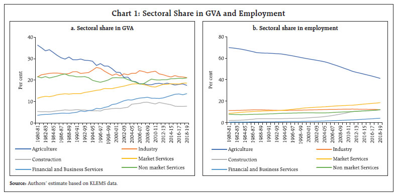 In terms of the productivity gap across sectors, it is observed that agricultural labour productivity in 2017-18 has been 0.67 times lower than the overall labour productivity of the economy. However, labour productivity in mining is observed to be higher due to higher capital intensity in the sector. Other sectors, where sectoral productivity is higher than the national average, include manufacturing, financial and business services and utilities. It is worth mentioning that the labour productivity in the financial and business services sectors is 5.5 times higher than the average labour productivity of the economy, whereas labour productivity in manufacturing is only 58 per cent higher than the average labour productivity. This indicates that there exists a large productivity differential across sectors (Chart 2). The income distribution across sectors shows that the average labour income share in construction is 40 per cent higher than in the agriculture sector (Table 1). In fact, the construction sector is considered to be a low-skill intensive sector and therefore, the sector provides an easy channel for agriculture workers to relocate. Migration from the agriculture sector to construction takes place due to higher wages in the latter with the same level of skill formation of the labourers. On the other hand, as industry is capital intensive in nature, the labour income share in the industry is much lower than the economy-level wage share. Within industry for manufacturing a declining trend in labour income share has been observed by few scholars (Goldar and Aggarwal 2005, Abraham and Sasikumar 2017, Goldar 2022). The structure of capital income in Table 1 shows that capital income is much higher in the industry as compared to the agriculture, construction, and services sectors. Further, the distribution of capital income in the industry increased in the 2010s compared to the decade of the 2000s. This suggests that the income distribution is favouring capital movement and attracting higher investment in the industrial sector, whereas labour income share in the industry remains stagnant. 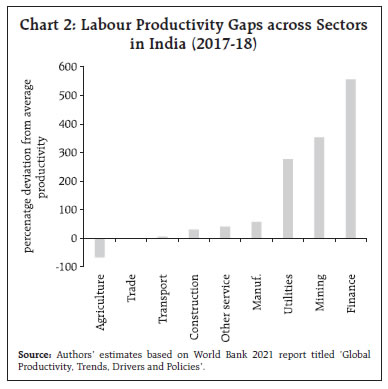
| Table 1: Relative Labour and Capital Income Share in Sectors | | Sectors | 2001-10 | 2011-19 | 2001-10 | 2011-19 | | Total Economy | 100 | 100 | 100 | 100 | | | Relative labour income share | Relative capital income share | | Agriculture | 132 | 126.8 | 77.1 | 79.4 | | Industry | 76.8 | 76.4 | 116.6 | 118.2 | | Construction | 185 | 176.4 | 39.3 | 41.2 | | Market Services | 101.6 | 105.9 | 98.8 | 95.5 | | Nonmarket services | 156.9 | 157.2 | 59.3 | 55.9 | | Source: Authors’ estimates based on KLEMS data. | As labour productivity gives a partial measure of productivity, we next discuss some trends in TFP across sectors. Table 2 provides the percentage change of employment, capital stock and TFP in 2011-19 over 2001-10. We find there is large heterogeneity among subsectors. For agriculture, we find positive TFP growth in 2010-19 over the previous subperiod. Within the low and medium-technology manufacturing sectors, the total factor productivity growth was observed to be the highest in sectors like textile and textile products, rubber and plastic products, coke & refined petroleum and other non-metallic mineral products. However, these sectors, which witnessed a large increase in productivity growth have registered declining growth of employment and capital during 2011-19 as compared to 2001-10. Thus, the sectors which are having large productivity are also witnessing labour displacement, which could lead to growth and reduce structural change. Similarly, within services, business services recorded a 4.8 per cent increase in productivity growth during 2011-19 as compared to 2001-10. The high productivity growth in business service sectors is again not associated with positive change in employment and capital growth, indicating resources are not moving to highly productive sectors. | Table 2: Change in Growth of Employment, Capital Stock and TFP; 2011-19 over 2001-2010 | | (Per cent) | | Sectors | Change in Emp Growth | Change in K stock growth | Change in TFP growth | | Agriculture, Hunting, Forestry and Fishing | -1.6 | -0.3 | 3.0 | | Mining and Quarrying | -2.8 | -1.2 | -0.2 | | Low and Medium Low-Tech Manufacturing | | Food, Beverages and Tobacco | -2.7 | -0.9 | -1.1 | | Textile and Textile Products, | -3.6 | -3.9 | 4.3 | | Leather and Footwear | | | | | Pulp, Paper products and footware, | -0.1 | -2.1 | 0.0 | | Printing and Publishing | | | | | Coke, Refined Petroleum | 2.4 | 1.9 | -4.6 | | Rubber and Plastic Products | -1.2 | -0.2 | 3.8 | | Other Non-Metallic Mineral Products | -5.1 | -4.8 | 5.9 | | Basic Metals and Fabricated Metal Products | -0.1 | -4.7 | 0.5 | | Manufacturing, nec; recycling | -5.6 | -5.7 | 6.8 | | High and Medium High-Tech Manufacturing | | Chemicals and Chemical Products | 0.6 | 2.2 | -2.7 | | Machinery, nec. | 3.0 | -3.2 | -3.5 | | Electrical and Optical Equipment | -0.5 | -4.4 | -5.6 | | Transport Equipment | -1.4 | -0.3 | 1.4 | | Market Services | | Trade | -0.7 | 7.6 | -1.1 | | Hotels and Restaurants | -2.3 | 1 | 2.2 | | Transport and Storage | -0.7 | 0.7 | -1.3 | | Post and Telecommunication | -3.5 | 7.3 | -9.5 | | Financial Services | -1.9 | -2.1 | -0.3 | | Business Service | -1.4 | -7.3 | 4.8 | | Non-Market Services | | Public Administration and Defense; | 1.6 | 0.3 | -2.4 | | Compulsory Social Security | | | | | Education | -1.0 | -0.7 | 4.0 | | Health and Social Work | -0.1 | -3.2 | -0.5 | | Other services | -0.3 | -2.4 | 2.3 | | Source: Authors’ estimates based on KLEMS data. | III. Empirical Method: Resource reallocation To empirically examine how much resource reallocation has contributed to productivity increase we use a growth accounting decomposition technique. Our methodology follows Jorgenson et al. (2007) decomposition approach and the data we use is taken from India KLEMS 2019 database. Methodology In this method, the aggregate production function is given as 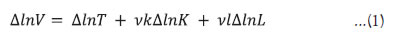 where ΔlnV denotes aggregate value-added growth. K and L represents inputs to the production function, viz. capital and labour. v represents two period average share of factor input compensation in nominal value added. vk denotes two period average of aggregate capital compensation in aggregate value added and vl denotes two period average of aggregate labour compensation in nominal value added. ΔlnK and ΔlnL denotes aggregate capital input and aggregate labour input growth rates. ΔlnT is the total factor productivity growth rates. The aggregate production function approach is considered restrictive due to some assumptions. Firstly, this approach assumes gross output of each industry is separable in value added. Secondly, output prices are considered identical across industries and thirdly, the heterogenous factor inputs receive same price across all industries. Given the limitations of aggregate production function, Jorgenson (2007) distinguishes between two other types of aggregation approach of production functions, which are production possibility approach and method of direct aggregation. The production function as per production possibility approach is given as where, aggregate value added is denoted by ΔlnVppf is translog aggregation of industry value added. K and L represent inputs to the production function, viz. capital and labour. The distinction between production function approach and production possibility approach is that the measurement of output changes from simple aggregation to translog aggregation but the measurement of inputs remains the same. Thus, the difference between (1) and (2) gives reallocation of value added. Next, we define the direct aggregation method as used in Jorgenson (2007). In direct aggregation, aggregate value added is assumed to be translog index of industry value added. However the production function at an industry level is a gross output-based production function given as industry j’s value addred to gross output ratio. Thus for the factor inputs Kj and Lj, weights reflect three components (a) share of industry value added in aggregate value added, (b) share of industry factor income in industry gross output and (c) share of industry value added in industry gross output. The bar over weights represents two period average. This equation helps to identify the origin of aggregate input accumulation effect from industry level. The weights in the last term of equation (7) gives Domer weights for TFP. As described above, equation (2) gives aggregate value added function, where inputs are simple summation across industries. On the other hand, equation (7) gives aggregate value added function, where inputs are weighted growth rates of industry labour and capital. Subtracting equation (2) from equation (7) and rearranging will give us the factor reallocation effects: 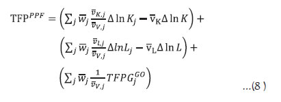 Equation (8) represents how the aggregate productivity growth from production possibility frontier relates to sources of growth at industry level. TFPPPF is the aggregate TFP growth derived from production psooibility approach. The first term of the right hand side of the equation denotes capital reallocation effects and and the second term captures the labour reallocation effects. The third term shows within industry contribution. The within industry contribution is calculated as weighted average of industry TFP growth. The weights of the TFP are Domar weights (Domar 1961). If aggregate TFP growth from PPF is greater than Domar weighted TFP growth in equation (8), the reallocation terms are positive. A positive reallocation term implies industries which pays higher input price have faster input growth. If reallocation term is positive, this would improve resource allocation and raise the aggregate TFP growth derieved from production possibility approach. Sources of Data: GVA and Factor Inputs The data for resource reallocation decomposition is based on India KLEMS dataset. The main advantage of KLEMS framework is factor inputs entering production function are measured more accurately by incorporating a quality index in input measurement. For instance, labour input is cross classified by educational attainment to account for productivity differences between low and high skilled labour services. Similarly, measurement of capital stock takes into account asset heterogeneity. In KLEMS dataset, the variables of output and factor inputs are constructed as follows: Gross value added and gross output data in KLEMS is constructed from National Accounts Statistics (NAS) published by NSO. For certain services sectors, Gross output estimates are not reported in NAS. In those cases, information is collected from various rounds of input output transaction tables (IOTT) published by NSO. Benchmark IOTT are used for 1993, 1998, 2003 and 2007, while for the intermediate years the ratios are interpolated linearly. The GVA/GO ratios calculated from IOTT tables are then applied to GVA series of NAS to obtain the GVO series of services sectors. Intermediate inputs which consist of material, energy and services are estimated from IOTT and adjusted with national accounts numbers at current prices. For constructing the series of intermediate inputs at constant prices wholesale price deflators are used which are obtained from the office of the Economic Advisor, Ministry of Commerce and Industry and appropriate weighted deflators are constructed using Balakrishnan & Pushpangadan (1994) method. The employment data is directly taken from KLEMS database. In this database, labour input data is estimated from employment unemployment survey (EUS) rounds and periodic labour force survey (PLFS) data. Employment and wage data are obtained as per skill level of workers defined by education categories. Data on wage rate for self-employed workers are obtained from India KLEMS by using Mincer equation (KLEMS manual 2021). Capital input data in KLEMS framework is estimated from NAS by obtaining investment data by asset type. Capital stock is estimated using perpetual inventory method, where depreciation rate for machinery is assumed to be 8 per cent. For construction depreciation is assumed to be 2.5 per cent and for transport equipment 10 per cent, respectively (KLEMS Manual 2021). The rental price of capital is external rate of return. IV. Results The results of the decomposition are shown in Table 3. The aggregate TFP estimates are derived from production possibility frontier approach. This aggregate TFP is then decomposed into within industry TFP effect calculated with direct aggregation approach (also known as Domar aggregation method) and reallocation effects. The analysis is done for two subperiods 2001-10 and 2011-19. The results show that aggregate TFP growth increased to 2.72 per cent in 2011-19 as compared to 1.33 per cent during 2001-10. What stands out is a remarkable difference in the structure of sources of aggregate TFP growth during the two sub periods. During 2000s (i.e.,2001-10) resource reallocation was the driver of aggregate productivity. Labour and capital reallocation together accounted for 82 per cent of aggregate productivity growth. Whereas in the second subperiod, factor reallocation contributed about 42 per cent of aggregate productivity growth. The aggregate productivity increase in the second subperiod originated from within industry productivity growth. When looked into the labour and capital reallocation effects separately, both the terms are found to be positive. A positive labour reallocation term would signify that prices of heterogenous labour differs across industries, and labour is moving towards sectors with high wages. If prices are considered as proxies for productivity, then this suggests movement of labour to high productivity sectors. It is observed from Table 3 that across both sub periods 2001-10 and 2011-19, capital reallocation effects were relatively lower than labour reallocation effects. Movement of workers from low wage agriculture to high wage non-agricultural sectors contributed to large positive labour reallocation effects. | Table 3: Aggregate Total Factor Productivity and Reallocation Effects | | Time Period | 2001 to 2010 | 2011 to 2019 | | 1. Aggregate TFP growth | 1.33 | 2.72 | | Contribution from | | 2. Within industry TFP growth | 0.21 | 1.58 | | 3. Reallocation effects | | | | a. Capital | 0.47 | 0.46 | | b. Labour | 0.66 | 0.68 | | Source: Authors’ estimates. | Another important finding from the above table is that aggregate TFP growth during the second subperiod (2011 to 2019) majorly reflects TFP growth in underlying industries. For instance, production possibility frontier based TFP for period 2011-19 was 2.72 per cent out of which 1.58 per cent was contributed from within industry TFP growth. Thus, it is important to study the within sector industry distribution of TFP. It is observed that TFP growth varies substantially across sectors (Chart 3). Within industries, labour intensive textiles and leather industries have high contribution to productivity growth. Other top performing sectors which contributed to productivity growth includes rubber and rubber products; import intensive coke and refined petroleum and parts and component producing sectors like transport and machinery equipment. Within services sectors, business and financial services contributes significantly to aggregate productivity growth. However, market services like trade and transport recorded a negative contribution to productivity growth. Overall, the within sector results suggests an increasing role of industry, financial services and non-market services in improving aggregate TFP and a declining role of market services in explaining TFP growth. 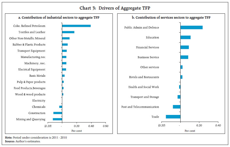 In terms of contribution of factor input reallocation on GVA growth, on an average, reallocation effects contributed to 5 percent of output growth during 2001 to 2019. A subperiod analysis shows that input reallocation contributed for around 8.0 per cent of GVA growth during 2011 to 2019, whereas within industry productivity growth accounted for 11.0 per cent of GVA growth during the same period. It is also observed that output growth in India is driven by factor input accumulation, where capital input explained around 65 per cent of output growth during 2011 to 2019 (Chart 4). V. Conclusion To conclude, we find that there exist large productivity differences across sectors. Agriculture, which employs the largest number of workers (around 41 per cent in 2018-19) is one of the lowest productive sectors – around 0.67 times lower than average productivity of the economy. Second, we find that reallocation of resources from low to high productive sectors accounted for 63 per cent of aggregate productivity growth during 2001-2019. A sub-period analysis shows that the aggregate total factor productivity growth increased from 1.33 per cent during 2001-10 to 2.72 per cent during 2011-19 mainly driven by within industry improvement in technological progress. A GVA growth accounting decomposition shows that resource reallocation effects contributed to 8.0 per cent of GVA growth during 2011 to 2019. During the second sub-period, aggregate productivity growth, however, was higher than the first sub-period and was driven by within sector productivity increase. The top performing sectors in terms of contribution to aggregate productivity in manufacturing included labour intensive industries like textiles, parts and component producing industries like machinery and transport, import intensive coke and refined petroleum. Within the services sector, financial and business services were the major drivers of aggregate productivity growth during 2011 to 2019. Reducing regulatory burdens can encourage new firms to enter the market and compete in the high productive sectors. Reducing subsidies including energy subsidies can help in redistribution of resource which is stuck in low productive and inefficient energy intensive sectors. Further, high productive sectors are becoming increasingly skill oriented. Higher investment in education, skill-based vocational training would also improve the ability of workers to move to high productivity sectors. Therefore, for encouraging efficient resource reallocation, policies should focus more on reducing market distortions, improve work force quality and managerial skills by investing in education, remove infrastructure bottlenecks and support research and development activities. References Abraham, V. and Sasikumar, S.K. 2017. Declining wage share in India’s organized manufacturing sector: Trends, patterns and determinants. ILO Asia-Pacific Working Paper Series, ILO, Delhi. Bartelsman, E., Haltiwanger, J., Scarpetta, S., 2013. Cross-country differences in productivity: the role of allocation and selection. Am. Econ. Rev. 103 (1), 305– 334. Bosworth, B., Collins, S.M., 2008. Accounting for growth: comparing China and India. J. Econ. Perspect. 22 (1), 45–66. Coe, D. T. 2007. Globalisation and Labour Markets: Policy Issues Arising from the Emergence of China and India. Organisation for Economic Co-operation and Development Social, Employment and Migration Working Paper 63. Paris: Organisation for Economic Co-operation and Development. de Vries, G.J., Erumban, A.A., Timmer, M.P., Voskoboynikov, I., Wu, H.X., 2012. Deconstructing the BRICs: structural transformation and aggregate productivity growth. J. Comp. Econ. 40 (2), 211–227. Denison, Edward F., 1967. Why Growth Rates Differ. Brookings, Washington, DC. Erumban, A. A., Das, D. K., Aggarwal, S., & Das, P. C. 2019. Structural change and economic growth in India. Structural Change and Economic Dynamics, 51, 186-202. Erumban, A.A., Das, D.K., 2016. Information and communication technology and economic growth in India. Telecommun. Pol. 40 (5), 412–431, http://dx.doi.org/10.1016/j.telpol.2015.08.006. Goldar, B. (2022). Impact of trade reforms on labour income share in Indian manufacturing. In Rajesh Raj S.N. and Komol Singha (eds), The Routledge Handbook of Post-Reform Indian Economy, Routledge, London and New York. Goldar, B. and Aggarwal, S. C. 2005. Trade Liberalization and Price-cost Margin in Indian Industries. The Developing Economies, September, Vol. 43, No.3, pp. 346-373 Havlik, P. 2005. Structural Change, Productivity and Employment in the New EU Member States. Wiener Institut für Internationale Wirtschaftsvergleiche Research Report 313. Vienna: Vienna Institute for International Economic Studies Hsieh, C.-T.; Klenow, P.J. 2009. “Misallocation and manufacturing TFP in China and India”, in Quarterly Journal of Economics, Vol. 124, No. 4, Nov., pp. 1403– 1448 Jorgenson, D.W., Ho, M.S., Samuels, J.D., Stiroh, K.J., 2007. Industry origins of the American productivity resurgence. Econ. Syst. Res. 19 (3), 229–252. Jorgenson, D.W., Timmer, M.P., 2011. Structural change in advanced nations: a new set of stylised facts. Scand. J. Econ. 113 (1), 1–29 Krishna, K.L, Erumban, A.A, Das, D.K, Aggarwal, S, Das, P.C 2017. Industry origin of economic growth and structural change in India, Working paper No 273, Centre for Development Economics. Kuznets, S., 1966. Modern Economic Growth: Rate, Structure and Spread. Yale University Press, London. Lewis, W.A., 1954. Economic development with unlimited supplies of labour. Manchester School Econ. Soc. Stud. 22, 139–191. Lin, J., 2011. New structural economics: a framework for rethinking development. World Bank Res. Observ. 26 (2), 193–221. Maddison, A., 1987. Growth and slowdown in advanced capitalist economies: techniques of quantitative assessment. J. Econ. Literat. 25 (2), 649–698. McMillan, M., Rodrik, D., 2011. Globalization, Structural Change, and Productivity Growth (NBER Working Paper 17143). NBER, Cambridge. Organisation for Economic Co-operation and Development (OECD) 2007a- OECD Employment Outlook. Paris: OECD Organisation for Economic Co-operation and Development (OECD) 2007b- Making the Most of Globalisation. OECD Economic Outlook 81. Paris: OECD Timmer, M.P., Dietzenbacher, E., Los, B., Stehrer, R., de Vries, G.J., 2015. An illustrated user guide to the World Input–Output Database: the case of global automotive production. Rev. Int. Econ. Timmer, M.P., Inklaar, R., O’Mahony, M., van Ark, B., 2010. Economic Growth in Europe: A Comparative Industry Perspective. Cambridge University Press. Vu, K.M., 2017. Structural change and economic growth: empirical evidence and policy insights from Asian economies. Struct. Change Econ. Dyn. 41, 64–77.
|