Timely and reliable information on crop production is a key element for gauging future inflationary trends. The study explores the utility of remote sensing data for policy analysis with a focus on pulses. Using satellite imagery-based Normalised Difference Vegetation Index (NDVI), vegetation growth is derived by suitable seasonal filtering and temporal aggregation. The results suggest that vegetation growth has significant ability to provide reasonably good assessment of commodity arrivals in mandis, well in advance. Further, geospatial modelling using location coordinates indicates the presence of spatial heterogeneity.

Introduction

Food Inflation has long been a focal point of policy debates in India. The Food and Beverages group, owing to its high weightage in the composition of Consumer Price Index (CPI) in India, exerts a high degree of price pressure on headline retail inflation. The effects may be persistent, with spillovers to other components as well as to inflation expectations, and therefore, warranting policy interventions.

Food inflation is influenced by a host of factors broadly categorised into demand-pull, supply-side, global and policy factors. These factors share a complex intrinsic structure, and their inter-dynamics shapes the inflation trajectory (Anand et al., 2016; Bhattacharya and Gupta, 2015; Sonna et. al., 2014). As food availability in the country is intrinsically shaped by domestic food production, with supply-side factors predominantly determining food availability, timely and reliable information on crop production becomes a key element in gauging future inflationary trends.

In India, Directorate of Economics and Statistics (DES) in the Ministry of Agriculture and Farmers’ Welfare (MoA&FW), Government of India (GoI) provides advance estimates of major food grains at the country level. Final country-level estimates are released after the crops are harvested¹. Moreover, the state and district-level crop production estimates are released with even a longer lag (one-two years) (DES, 2020).

Publication delays in official data has led to the exploration of alternative sources, such as high frequency remote sensing data. Availability of spatio-temporal remote sensing data at high-frequency and near real-time basis provides an extra edge over traditional datasets and is being explored extensively. With modern big data tools, machine learning and image processing capabilities, the usage of remote sensing data has become even more appealing. The related literature suggests that satellite imagery-based vegetation indicators have the potential to capture change patterns on earth which can be valuable for monitoring of agricultural crop production and estimating crop yields.

The wholesale and retail prices are influenced by commodity prices recorded in agricultural markets (mandis), which typically represent an initial touch point for transaction by farmers and traders, and thus, prices at the first level of transaction. Mandi prices primarily depend on arrival quantity, though there could be additional factors such as procurement policy, export/import decisions and minimum support prices influencing the mandi prices. A timely assessment of arrivals is crucial as lower arrivals may build price pressures. Mandi arrivals and prices are also analysed while making nowcast for retail inflation (Raj et al., 2019).

Against this backdrop, the article explores the utility of remote sensing data for policy analysis with focus on pulses, especially Tur. The choice of Tur is motivated by two factors: (i) India is one of the largest producers and consumers of pulses globally, (ii) retail inflation is seen to be sensitive to Tur, as the latter carries the highest weight (33 per cent) in pulses sub-group. The overall analytical approach and modelling framework is kept simple in order to (i) be able to deploy it in an operational environment, (ii) to keep the scope of scalability (to cover more geographical regions and additional indicators) and replicability (to cover other commodities) open.

Using the satellite imagery-based Normalised Difference Vegetation Index (NDVI), vegetation growth is derived by suitable seasonal filtering and temporal aggregation. Vegetation growth, an indicator of crop production, provides an assessment of commodity arrivals in mandis in advance. Rainfall data is also used as additional variable for robustness check and efficiency gain.

The article makes a useful contribution to the literature. First, a direct study of the inter-linkages between vegetation indicators and mandi arrivals is a departure from the existing studies that look at crop yield estimation. Moreover, this approach brings us one step closer to inflation assessment. Second, experimenting with geospatial models for understanding spatial heterogeneity is relatively limited in extant studies.

Our results suggest that vegetation growth has significant ability to provide reasonably good assessment of commodity arrival growth in mandis, well in advance. Vegetation growth influences the growth in mandi arrivals positively and strengthens as the season progresses. The effect of vegetation indicator is found to be stronger than rainfall for our period of study. Geospatial modelling using location coordinates indicates the presence of spatial heterogeneity.

The rest of the article is structured as follows. Section II presents a brief review of relevant literature. The representative area and datasets used in the article have been discussed in Section III. In Section IV, we present stylised facts and discuss first stage results which set the basis for the next section. Section V sets out the modelling framework. Empirical results are presented and discussed in Section VI. Section VII concludes with future proposals.

II. Review of Literature

An enhanced access of earth observation data has created opportunities for downstream applications and innovations in various domains. Satellite data offers multi-faceted applications and are being used for several purposes, including but not limited to, agriculture, environmental dynamics, security and defense activities, demographic characteristics, urbanisation, public policies, disaster management and monitoring the progress of sustainable development goals (Donaldson and Storeygard, 2016; Goldblatt et al., 2019; OECD, 2020; World Bank, 2017).

Globally, agriculture has been a core application area of remote sensing. In India, agriculture has been a major driver for the Indian Space Programme, starting with the Coconut Wilt Experiment in 1969 to the cutting-edge experiments and multi-faceted applications of today. Satellite imagery has been used successfully in precision agriculture, crop production/ yield assessment, land cover estimation, climate change impact, drought and horticulture (Ray, 2016; Navalgund and Ray, 2019).

Agricultural ecosystems are complex and crop conditions are influenced by a host of factors, both climatic (precipitation, temperature, soil moisture) and agronomic practices (sowing timing, seed quality, cropping pattern, fertilizer, pesticide, farming practices). Vegetation indices represent the crop conditions in near real time accounting for various factors and are significant inputs in yield / production forecasting models (Johnson et al., 2016)².

The selection of representative regions is based on the varieties of crops produced in a country. Accordingly, studies focus on specific crops and consider the representative regions producing these crops, though they may vary in their approach and model designs (Dubey et al., 2018; Johnson et al., 2016; Rembold et al., 2013; Manjunath et. al., 2002). In the literature, it is a general practice to derive a measure of vegetation condition by suitable transformation or aggregation of NDVI values, for assessing changes in vegetation patterns. Due attention is also paid to capture the phenological stages of the crop while doing so (Balaghi et. al., 2008; Johnson, 2014; Gumma et al., 2021; Wall et al., 2008; Mkhabela et al., 2011; Panek and Gozdowski, 2020).

Linear regression using ordinary least squares (OLS) is a common method adopted in most studies. A relatively new dimension in this area aims at examining presence of spatial variability using Geographically Weighted Regression (GWR) framework. GWR has found applications in agricultural domain, though the references are rather limited (Haghighattalab et al., 2017).

Most studies focus on target crop yield estimation and anomaly detection. Very few empirical studies have directly examined the inter-linkages between vegetation indicators and mandi arrivals/prices, as we have attempted in this article.³

III. Representative Region and Data

III.1 Representative Region

India is a geographically vast country with diverse topography, multiple crops, varying climatic conditions and multiple seasons. Considering these features, a simple aggregation of regions may dilute the rich micro-information from disaggregated data. Therefore, the selection of representative regions, which are significant for the target crop of Tur, assumes significance.

Tur production in India is regionalised. Three states - Karnataka, Madhya Pradesh and Maharashtra – have contributed about 60-70 per cent in the all-India Tur production in the recent period (2015-16 to 2019-20), commanding a similar share in area coverage. Top 15 districts from these three states having 40-45 per cent share in all-India production are selected for the current study (Chart 1).

III.2 Data

A range of datasets are used in this study covering mandi arrivals, remote sensing vegetation and rainfall data; the period is from 2012 to 2021. Temporal signatures depend on the crop being analysed. Due to seasonality, the selection of appropriate time windows for modelling assumes importance. As vegetation data are available at fortnightly frequency, mandi arrival and rainfall data are aggregated on a fortnightly basis.

III.2.1 Mandi Arrival Data

Commodity arrivals at agricultural markets (mandis) influence mandi prices, which represent the first stage in the price setting mechanism, and impact wholesale price and retail prices in subsequent periods. Daily data on mandi prices and arrival quantity are published on the Government portal Agricultural Marketing Information Network⁴.

In line with the objective of this study, daily data of Tur for all the mandis of select three states were collected. Though the data are available at daily frequency, there are instances of missing values, which vary across mandis. Therefore, a filtering mechanism was adopted to exclude mandis having missing data more than a threshold value. For remaining mandis, missing data, if any, were imputed using the Kalman Filter method.

Mandi prices depend on commodity arrivals not only in the same time period, but also on arrivals during the first few months following the crop harvesting period. Accordingly, cumulative arrivals are derived for each fortnight in year-to-date manner and arrival growth is computed (for the same fortnight a year ago).

III.2.2 Remote Sensing Vegetation Data

The multispectral remote sensing captures image data within specific wavelengths across the electromagnetic spectrum. A color composite is obtained by the combination of different bands, highlighting the presence of vegetation and distinguish it from other features (water, soil, manmade features). Vegetation appears differently at visible red (RED) and near-infrared (NIR) wavelengths and this insight of varying reflectance is used to construct the vegetation index.

The Normalised Difference Vegetation Index (NDVI), derived from the satellite imagery of crops, is the most widely used vegetation indicator in agriculture remote sensing literature; it is illustrated below. NDVI is range bound and a higher value indicates healthier vegetation. Temporal changes in NDVI value indicate changes in crop vigor and used for monitoring crop growth in progressive manner.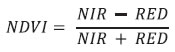

Generally, crop production data are available at a particular administrative level (e.g., district in India), and hence to develop a model, NDVI is aggregated in a manner such that it represents the vegetation of the administrative region (Dubey et al., 2018; Balaghi et al., 2008; Panek and Gozdowski, 2020). As there could be one or more mandis located in one district, using NDVI at district level may not be appropriate as it may dilute the results. Accordingly, NDVI at sub-district level (Taluk or Tehsil), is considered. This one-step drill-down offers advantage in terms of maintaining the inherent information contained in granular data and offers a way to map the production area to mandis at the same time⁵. In the present study, MODIS NDVI 16-Day L3 Global “MOD13A1” dataset is used, sourced from Indian Space Research Organisation (ISRO) VEDAS web-portal (Visualization of Earth Observation Data and Archival System). This data is available at fortnightly frequency.

For modelling of arrival growth, NDVI also needs suitable transformation in order to represent the year-on-year growth in vegetation. Further, it is not known a priori which fortnight during the growing season would be optimal for a fair representation of the production, as the timing may vary from one location to another and / or from one year to another (depending on the sowing timing or climatic factors). Therefore, a suitable temporal aggregation of NDVI during the growing season is desirable representing the cumulative effect in line with literature, which would also be in sync with cumulative arrivals being used in the study.

Tur is mainly cultivated in semi-arid regions and can tolerate drought to a certain extent. It needs water at the time of sowing, but unusual heavy rains at later growth stages can be destructive for the crop. Tur being a Kharif crop, the season starts with sowing at onset of monsoon (June and July), growing period of 3-4 months (August, September, October, November) and harvesting begins in late November or early December, which may vary slightly from region to region (Tiwari and Shivhare, 2017; GoI, 2020).

Accordingly, the NDVI values for successive fortnights are aggregated and cumulative NDVI (CNDVI) is derived for each fortnight during the growing months. Vegetation growth is represented as annual growth in CNDVI (same fortnight a year ago)⁶.

III.2.3 Rainfall Data

In addition to remote sensing information, land-based measurements, particularly rainfall data are also analysed. In India, rainfall is primarily recorded during the South-West Monsoon (SWM). It acts as a precursor to the sowing activity and is a key determinant of Kharif crop production (RBI, 2015). We include it for robustness check and for possible improvement in the explanatory value of the model.

Daily data on rainfall, current and historical normal rainfall, captured by Indian Meteorological Department (IMD), sourced from India Water Resources Information System (WRIS), is used for the analysis. Rainfall deviation has been derived as departure of actual rainfall from historical normal rainfall for each fortnight. These data are not available at Taluk level, and therefore, district-level data have been considered.

IV. Stylised Facts

Salient features of data are presented in this section, which help in understanding the seasonal dynamics as a prelude to the modelling exercise. Chart 2 presents cumulative NDVI of different Taluks in Karnataka state in the second fortnight of October for two sample years, which clearly depicts variation in vegetation conditions across Taluks and also between years.

Post harvesting, the commodity starts slowly arriving at the mandis in December, picks up in January and February and tapers slowly afterwards. A large part of the arrivals happens in a few months, approximately 40-50 per cent during the first three months (December to February) and 70-80 per cent during first 6 months (December to May) (Chart 3).

Taking cognisance of the strong seasonal influence, data pertaining to the peak of season has been considered for analysis, as indicated in Chart 4. It is logical considering that a crop can be produced only during a particular season, but its influence on arrivals may be measured over a period of time.

The changes in production should ideally be reflected in subsequent arrivals, and it is expected that a higher (lower) growth in vegetation gives an indication of higher (lower) arrivals in mandis. Chart 5 presents trend in cumulative NDVI growth (October second fortnight) and cumulative arrival growth (May-end) during the period under study.

The scatter plot shows a positive linear relationship, i.e., when vegetation growth becomes higher, so does the arrival growth. Similarly, poor growth in vegetation coincides with lower growth in arrivals. It is also able to capture the bad and good years reasonably well (bad and good years defined as per production data sourced from DES).

Though the crop sowing area may remain broadly the same, vegetation vigor and growth may change quickly during the growing season. Correlation between rainfall deviation, vegetation growth and arrival growth are derived at various fortnights and presented in Chart 6.

The correlation signs are as expected. Vegetation growth influences arrival growth positively, while rainfall deviation impacts crop production negatively, and hence, the subsequent arrivals. Correlation of arrival growth with vegetation growth is strong and consistent throughout the season, while correlation with rainfall deviation is much smaller in magnitude and significant only for one fortnight viz., the first fortnight of July, while other patterns are inconsistent. This is not surprising given the fact that the sowing season of Tur is in June and July when the rains can affect production, whereas vegetation across the entire growing season can influence the arrivals in near future.

V. Modelling Framework - Arrival Growth

Preliminary results in Section IV provide encouragement for the development of arrival growth model based on vegetation growth. Along with single indicator models, hybrid model using both vegetation and rainfall information are also developed, for robustness check and any incremental value that they may provide. As crop conditions may change during the growing cycle, the influence is estimated dynamically at different time points in the growing season. Model specifications are presented below:

where, ARG_f is arrival growth for fortnight f, RFD_r is rainfall deviation for fortnight r and VEG_k is vegetation growth for fortnight k, as defined earlier in Section III, and fortnights are indicated as below:

f = arrival fortnight = 1 to 12 = December first fortnight to May second fortnight,

r = rainfall fortnight = 3 = July first fortnight,

k = NDVI fortnight = 1 to 8 = August first fortnight to November second fortnight

Keeping the structure same, the models are trained separately for different fortnights of arrivals and NDVI⁷. It enables us to understand how the coefficient evolves during the season and how incremental gains are made in terms of explanatory power in a progressive manner.

The vegetation coefficient β is expected to be positive, and rainfall deviation coefficient γ is expected to be negative. Further, the value of coefficient β, at different k, may be viewed as the changing influence of vegetation growth on arrival growth (of a specific arrival fortnight). It is expected that, as the season progresses, β strengthens in magnitude. A significant positive coefficient early in the season would be an added advantage, as arrival growth could be assessed even before harvest.

Another dimension to examine is how the vegetation coefficient β changes from NDVI model (eq. 2) to Hybrid model (eq. 3), when rainfall deviation is added. If the estimated values of β are similar in both models, it implies that rainfall does not add much value in explaining arrival growth. A similar interpretation is possible for rainfall coefficient γ as well. In addition to coefficients, one may look at the changes in model R-square or information criteria for a comparative perspective.

V.1 Geospatial Modelling

In the OLS regression models, the intercept (α) and slope coefficient (β) are constant for all locations in the study area. However, in reality, the inter-linkages between the explanatory variables (rainfall deviation and vegetation growth) and dependent variable (arrival growth) may vary from one location to another (depending on climatic factors and geographical features), and therefore a uniform relationship as measured by OLS may not be appropriate. Deciphering the presence of spatial variability may lead to interesting geographical patterns and relationships, which otherwise might be known to domain experts but not available empirically.

While undertaking spatial analysis, it is essential to understand and incorporate the geographical features. Tobler’s First Law of Geography states “Everything is related to everything else but near things are more related than distant things” (Miller, 2004). This concept provides an intuitive basis for analysing geographical similarity or variation. As conventional statistical models may not be able to capture geographical heterogeneity, Geographically Weighted Regression (GWR) models are developed and used (Brunsdon et al., 1996; Fotheringham et al., 2002). Spatial analysis is performed using GWR model, technical details on which have been provided in Annex.

VI. Empirical Results

We train various models as outlined in Section V. For a particular fortnight (f) of arrival, there are eight vegetation coefficients (β) pertaining to the eight fortnights (k) of NDVI (August first fortnight to November second fortnight). Similarly, there would be one coefficient (γ) of rainfall deviation corresponding to the 3rd fortnight (July first fortnight). Data upto May 2020 is used for training the models, while remaining data are kept aside for evaluation.

VI.1 OLS model results

Several interesting results are obtained, key results are highlighted and discussed in subsequent paragraphs for select arrival fortnights.

i. Impact of vegetation on arrivals is strong and robust - The vegetation growth influences arrival growth positively and its influence consistently strengthens as the season progresses. Its impact peaks by the end of October and stabilises thereafter. Vegetation coefficients are robust, as addition of rainfall does not seem to alter its value (Chart 7). The upward pattern remains broadly same for various arrival fortnights.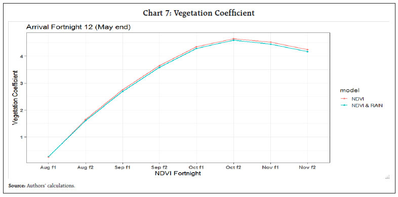

ii. Vegetation indicator provides a fair assessment of arrivals, while rainfall impact is negligible - A comparative assessment of individual and combined models, in terms of Adjusted R-square and Bayesian Information Criterion (BIC), reveals interesting facts. While the variability in arrival growth is explained reasonably well by vegetation growth, depicting progressive improvement and stable relationship, standalone rainfall model fails to explain any variation. Further, the individual NDVI and NDVI with RAIN models are very close, indicating that addition of rainfall does not provide any material gain, beyond the variation explained by vegetation during the period under study (Chart 8).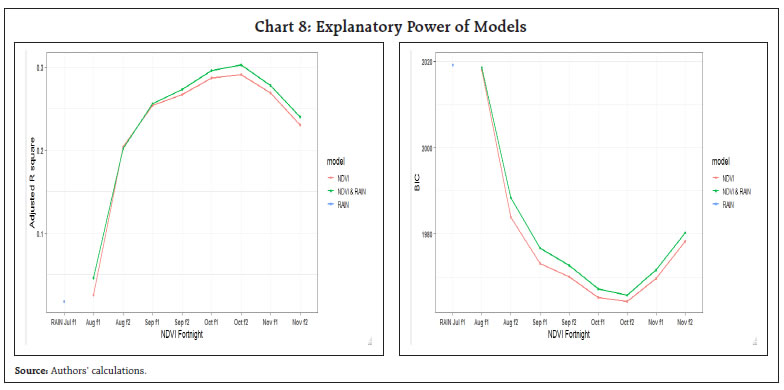

iii. Early-on contribution of vegetation is significant - During the entire growing season, from August to November, sequential improvement in the inter-linkage between vegetation growth and arrival growth is seen (Chart 8). The significance of coefficients of vegetation growth in early fortnights, as early as September first fortnight, which sees a significant jump from August first fortnight and is closer to the maximum influence as seen in October second fortnight, is a key result (Chart 7).

iv. Model projections provide early information for identification of a good or bad year - NDVI model-based arrival growth projections are in line with actual patterns, lower in bad years and higher in good years, re-confirming the utility of remote sensing data for assessment arrival growth well in advance (Chart 9).

VI.2 GWR model results

GWR models are developed for NDVI model only, as rainfall effect is found to be negligible, as seen in Section VI.1. Spatial dimension of elements in the space (mandis) is represented by their corresponding latitude and longitude coordinates, based on which the proximity between elements is derived. For brevity, we present results pertaining to the second fortnight of February, which accounts for approximately 50 per cent of total arrivals in a year. It is based on vegetation growth corresponding to October second fortnight, which has maximum explanatory power in the estimated OLS model.

Localised parameter estimates for vegetation growth are presented in Chart 10 (A to C) for visual clarity and distinction. It is observed that relationship between vegetation growth and arrival growth is stronger for mandis in Karnataka and Madhya Pradesh than in Maharashtra.

The local parameter estimates of GWR model are compared with the global estimate (equivalent to OLS estimate). The results are presented in Table 1, which indicate variation in coefficient values.

Though the heterogeneity in location-wise estimates can be seen in Chart 10 and Table 1, we need to test if the spatial variation in estimates across the study area is statistically significant. Following Leung et al. (2000), the null hypothesis of parameter equality i.e., all local coefficients are equal is tested, against the alternative hypothesis of not all local coefficients are equal. The null hypothesis (at one per cent level of significance) is rejected confirming the presence of heterogeneity in parameter estimates for Vegetation Growth (β) (Table 2).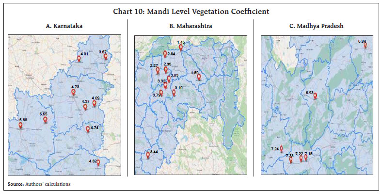

In order to examine the performance of GWR and OLS, the ANOVA test suggested in Brunsdon et al. (1999) is used. The goodness-of-fit of OLS model is compared with GWR and the improvement obtained by the GWR model is examined. The test results are presented in Table 3. The ANOVA results suggest that the gain obtained by using GWR is significant, and the null hypothesis of adequacy of OLS model is rejected in favour of GWR model (at 10 per cent level of significance).

VII. Conclusions and Way Forward

Crop growth is a potential source of advance information for assessing the arrivals in mandis, which in turn could influence the future trends in wholesale and retail prices. This article combines remote sensing and ground-based indicators to develop an empirical approach to predict agricultural commodity arrivals in mandis prior to the harvest. It uses a regression-based model embedded with appropriate seasonal filtration and optimised for capturing spatial heterogeneity (geographically-weighted regression).

Due emphasis has been given to select representative regions (districts) for the target crop (Tur), considering the production of multiple crops and diverse topography of India. Vegetation indicators pertaining to sub-district level (taluk) in the selected districts have been used to exploit granular information.

The dynamic approach using sequentially updated vegetation growth values enables us to (i) monitor crop conditions on a near real-time basis, (ii) study how the relationship between NDVI and arrivals evolves during the season and (iii) re-assess the arrival growth as and when new data become available. The crop coefficients, estimated early in the season, provide confidence for planning and policy making.

The influence of vegetation growth on arrival growth is found to be significant and robust, which strengthens as the season progresses. It is stronger than the effect of rainfall deviation and varies across locations. The results uphold the use of remote sensing data as a surveillance tool for agro-commodities and projections in near future. The utility is further enhanced by the early availability of vegetation indicators.

To sum up, the analysis in this article has considerable policy use. It can be further strengthened in many ways, going forward. First, in addition to vegetation indicators, climatic factors can be included.

Secondly, factors affecting arrivals, such as crop damage during harvesting, transportation or storage, imports, pricing and demand situation, can also be considered while developing an optimal prediction model for arrivals. Thirdly, vegetation indicators can be incorporated in a forecasting framework for inflation, along with other indicators. Finally, following recent advancements by remote sensing experts, high resolution images at fine grid levels supported by ground truth data, sophisticated image analytics, and machine learning algorithms can be used to identify the exact crop and forecast production.

References

Anand, R., Kumar, N. and Tulin, V. (2016). Understanding India’s Food Inflation: The Role of Demand and Supply Factors, IMF Working Paper No. 16/2

Balaghi, R., Tychon, B., Eerens, H., Jlibene, M. (2008). Empirical Regression Models using NDVI, Rainfall and Temperature Data for the Early Prediction of Wheat Grain Yields in Morocco, International Journal of Applied Earth Observation and Geoinformation 10, 438–452

Bhattacharya, R. and Gupta, A. S. (2015): Food Inflation in India: Causes and Consequences. National Institute of Public Finance and Policy (NIPFP) Working Paper No. 2015-151, June.

Bivand, R. and Yu, D. (2007). SPGWR - Geographically weighted regression. Available online at https://cran.r-project.org/web/packages/spgwr/index.html, accessed November 23, 2021

Brunsdon, C., Fotheringham, A. S. and Charlton, M. E. (1996). Geographically Weighted Regression: A Method for Exploring Spatial Nonstationary. Geographical Analysis, Vol. 28, 281-298

Brunsdon, C., Fotheringham, A. S. and Charlton, M. (1999). Some Notes on Parametric Significance Tests for Geographically Weighted Regression, Journal of Regional Science, Vol. 39, No. 3, 1999

Donaldson, D. and Storeygard, A. (2016). The View from Above: Applications of Satellite Data in Economics, Journal of Economic Perspectives, Vol. 30, No. 4, 171-198

Dubey, S. K., Gavli, A. S., Yadav, S. K., Sehgal, S. and Ray, S. S. (2018). Remote Sensing-Based Yield Forecasting for Sugarcane Crop (Saccharum officinarum L.) in India, Journal of the Indian Society of Remote Sensing, 46(11), 1823-1833

DES (2020). Agriculture Statistics at a Glance 2019, Directorate of Economics and Statistics, Department of Agriculture, Cooperation and Farmers Welfare, Ministry of Agriculture and Farmers Welfare, Government of India, available at https://eands.dacnet.nic.in/

Fotheringham, A. S., Brunsdon, C. and Charlton, M. (2002). Geographically Weighted Regression: The Analysis of Spatially Varying Relationships. Wiley, New York

Goldblatt, R., Monroe, T., Antos, S. E. and Hernandez, M. (2019). Innovations in Satellite Measurements for Development, World Bank Blogs, January

Government of India (2020). Biology of Cajanus Cajan (Pigeon Pea), Ministry of Environment, Forest and Climate Change (MoEF&CC) and Indian Institute of Pulses Research, Kanpur

Gumma, M. K., Kadiyala, M. D. M., Panjala, P., Ray, S. S., Akuraju, V. R., Dubey, S, Smith, A. P, Das, R. and Whitbread, A. M (2021). Assimilation of Remote Sensing Data into Crop Growth Model for Yield Estimation: A Case Study from India, Journal of the Indian Society of Remote Sensing, 46(11), 1823-1833

Haghighattalab, A., Crain, J., Mondal, S., Rutkoski, J., Singh, R. P., and Poland, J. (2017). Application of Geographically Weighted Regression to Improve Grain Yield Prediction from Unmanned Aerial System Imagery. Crop Science, Vol. 57, 2478-2489

Johnson, D. M. (2014). An Assessment of Pre and Within Season Remotely Sensed Variables for Forecasting Corn and Soybean Yields in the United States, Remote Sensing of Environment, 141

Johnson, M. D., Hsieh, W. W., Cannon, A. J. and Davidson, A. (2016). Crop Yield Forecasting on the Canadian Prairies by Remotely Sensed Vegetation Indices and Machine Learning Methods, Agriculture and Forest Meteorology, 218-219

Leung, Y., Mei, C. M. and Zhang, W. X. (2000). Statistical Tests for Spatial Nonstationarity Based on the Geographically Weighted Regression Model, Environment and Planning, Vol. 32, 9-32

Manjunath, K. R., Potdar, M. B. and Purohit, N. L (2002). Large Area Operational Wheat Yield Model Development and Validation based on Spectral and Meteorological Data, International Journal of Remote Sensing, Vol. 23, No. 15, 3023-3038

Mkhabela, M. S., Bullock, P., Raj, S., Wang, S. and Yang, Y.(2011). Crop Yield Forecasting on the Canadian Prairies using MODIS NDVI data, Agricultural and Forest Meteorology, Vol. 151, No. 3, 385-393

Miller, H. J. (2004). Tobler’s First Law and Spatial Analysis. Annals of the Association of Americal Geographers, 94(2), 284-289

OECD (2020). Measuring the Economic Impact of the Space Sector. Background Paper for the G20 Space Economy Leaders’ Meeting (Space20), October

Panek, E. and Gozdowski, D. (2020). Analysis of relationship between cereal yield and NDVI for selected regions of Central Europe based on MODIS satellite data, Remote Sensing Applications: Society and Environment, 17

Prasad, G., Vuyyuru, U. R. and Gupta M. D. (2018). Agricultural Commodity Arrival Prediction Using Remote Sensing Data: Insights and Beyond, KDD Fragile Earth Workshop

Raj, J., Kapur, M., Das, P., George, A. T., Wahi, A. and Kumar, P. (2019). Inflation Forecasts: Recent Experience in India and a Cross-country Assessment, Reserve Bank of India Mint Street Memo No. 19

Ray, S. S. (2016). Remote Sensing for Agricultural Applications, GeoSmart India, Geomatics for Digital India, March

Reserve Bank of India (2015). Monsoon and Indian Agriculture - Conjoined or Decoupled, RBI Monthly Bulletin, May

Rembold, F., Atzberger, C., Savin, I. and Rojas, O. (2013). Using Low Resolution Satellite Imagery for Yield Prediction and Yield Anomaly Detection, Remote Sensing, 5, 1704-1733

Sawasawa, H. L. A. (2003). Crop Yield Estimation: Integrating RS, GIS, Management and Land Factors, International Institute for Geo-Information Science and Earth Observation Enschede

Sonna, T., Joshi, H., Sebastian, A. and Sharma, U. (2014). Analytics of Food Inflation in India, RBI Working Paper Series No. 10/2014, October

Navalgund, R. R. and Ray, S. S. (2019). Application of Space Technology in Agriculture: An Overview, Smart Agri Post, 6(6), 6-11.

Tiwari, A. K. and Shivhare, A. K. (2017). Pulses in India: Retrospect and Prospects, Directorate of Pulses Development, MoA&FW, GOI

Wall, L., Larocque, D. and Leger, P-M. (2008). The Early Explanatory Power of NDVI in Crop Yield Modelling, International Journal of Remote Sensing, Vol. 29, No. 8, 2211-2225

World Bank (2017). Using Satellites to Monitor Progress towards the SDGs. World Bank News, August

Xue, J. and Su, B. (2017). Significant Remote Sensing Vegetation Indices: A Review of Developments and Applications, Hindawi Journal of Sensors, Article ID 1353691

Annex: Geospatial Modelling – Brief Technical Details

GWR allows the relationship (parameters estimates) to change across various locations in space and thus provides a basis for analysing spatial variability. GWR model is calibrated in a way that it produces location specific parameter estimates directly. The GWR model is expressed as an extension of OLS model form, as below -

where α(u_i, v_i) and β(u_i, v_i) represent the local coefficients, as a function of location coordinates (u_i, v_i) which adds spatial dimension to the regression model. Weighted least square method is used for estimation of parameters, with a diagonal weighting matrix where each diagonal element corresponds to weighting scheme for a particular observation location (Brunsdon et al., 1999; Leung et al., 2000).

Nearby locations are assumed to have more influence and hence assigned more weight compared to faraway locations (this is possibly based on “distance decay” concept in geography). For each observation at location i, the weight of another observation at location j depends on its distance from location i and the weighting function can take any of the following forms -

where d_ij is the spatial distance between location i and j, and h is the bandwidth which controls the degree of distance decay. The bandwidth can be fixed for all observations, or adaptive kernel, which allows the bandwidth to be larger when data is sparse and smaller when data is dense. We use bi-square weighting scheme with adaptive kernel suitable for smaller sample size and bandwidth optimisation is done using corrected Akaike Information Criterion (AIC).

Once the GWR model calibration is complete, statistical tests may be used to check whether (i) GWR performance is better than OLS and (ii) differences in parameter estimates are significant. The underlying idea is to examine whether the improvement in model fit provided by GWR over OLS is genuine and not arbitrary. Brundson et al., 1999 and Leung et al., 2000 provide detailed discussion and methods for GWR related hypothesis testing, addressing several theoretical issues.

* This article is prepared by Shweta Kumari and Sandhya Kuruganti of Big Data Analytics Division, Department of Statistics and Information Management, Reserve Bank of India. The authors express their gratitude to Ajit Ratnakar Joshi for his encouragement and valuable guidance. Views expressed in the article are those of the authors and do not represent the views of the organisation they belong to.

¹ Under the FASAL scheme (Forecasting Agricultural Output using Space, Agro-meteorology and Land based observations), pre-harvest forecasts of acreage and production are generated for selected ago-commodities using multiple data sources. The scheme is operated by Mahalanobis National Crop Forecast Centre (MNCFC), MoA&FW, in collaboration with Indian Space Research Organisation, India Meteorological Department, State Agriculture Departments, Institute of Economic Growth and Agricultural Universities. (DES, 2020; Ray, 2016).

² In satellite crop monitoring, there are a host of indicators for measurement of vegetation vigor, using different combination of spectral bands, such as Normalised Difference Vegetation Index (NDVI), Ratio Vegetation Index (RVI), Leaf Area Index (LAI), Soil Adjusted Vegetation Index (SAVI), Difference Vegetation Index (DVI) and Enhanced Vegetation Index (EVI). Though these vegetation indices may be useful for specific applications, NDVI has been a common choice in empirical studies and for operational applications (Xue and Su, 2017; Sawasawa, 2003).

³ A related paper in this regard is by Prasad et al. (2018) that predicts arrivals using NDVI data of neighborhood locations for select regions of Karnataka.

⁴ See www.agmarknet.gov.in

⁵ In order to link production to arrival, each taluk is mapped to its nearest mandi within the same district. Spherical distance between a taluk and mandi is measured by using Havershine method based on latitude-longitude co-ordinates.

⁶ NDVI values and other transformation of NDVI, such as vegetation condition index (min-max normalisation) and standardised z-score based on historical values were also analysed. However, their correlations with arrival growth were low and insignificant and hence have not been included here.

⁷ Data of 25 mandis for various years during the study period is used in the analysis and OLS models were developed with pooled data. Separate models may be developed for individual mandis, though it would need sufficient data for robust parameter estimates and as the sample size is limited, this was not attempted.