The coincident index (CI)1, constructed based on four daily indicators, captures the real-time momentum in economic activity at sub-national as well as national level. CIs across all regions plunged downward sharply following the lockdown in last week of March, reflecting sharp fall in the economic activity. CIs momentum shows that different regions have observed a varying pace of recovery with the gradual unlocking of the economy starting from June 2020. Notably, CIs for states in all regions registered sharp upturn in October. Though some moderation was recorded in the first half of November, momentum remained positive and reversed in second-half in most states. Furthermore, all-India CI has robust positive and statistically significant relationship with growth in industrial output. Introduction Monitoring economic activity through high frequency indicators has become paramount for the proactive public policy over the years. During normal times, the economic indicators with monthly and quarterly frequency, such as industrial activity, automobile sales, cargo handling and air passenger traffic, etc., are used to capture the underlying evolving economic impulses. But monthly and quarterly frequency indicators are unable to provide the required granular real-time information about the swiftly evolving economic dynamics during the period that is characterized by high level of uncertainty and rapid changes. In recent times, the COVID-19 pandemic period has been such that the economic activity witnessed a cliff event with sharp contraction across the board, reflecting stringent containment measures including lockdown. Even publishing regular data became a challenging task during the COVID-19 pandemic due to technical and logistical issues. Hence, COVID-19 pandemic has completely altered how policymakers monitor economic data due to rapidly evolving economic activity with shortened policy response time and diverging sub-national trends. Since economic changes have been rapid and profound during COVID-19 pandemic, real-time spatial information on the economic activity became critical to draw appropriate inferences for swift and nimble-footed policy decisions. In this context, coincident indices (CIs) based on high frequency data have come in handy to gauge the momentum in economic activity during the COVID-19 pandemic (Federal Reserve Bank of Philadelphia2 and Federal Reserve Bank of New York3). CIs are computed by combining indicators over time and space. The Federal Reserve Bank of New York uses ten indicators with weekly frequency to constitute weekly economic index (WEI), while the Federal Reserve Bank of Philadelphia combines four state-level variables to construct a monthly coincident index for each of the 50 states. Economic activity in India plunged in the first quarter (Q1) of 2020-21 with stringent nationwide lockdown imposed in the last week of March and extended subsequently. This resulted in Indian economy registering its sharpest decline of 23.9 per cent in real GDP during Q1:2020-21. The gradual unlocking process began in the first week of June 2020 and thereafter, economic activity started gaining some momentum. In Q2:2020-21, states also implemented localised lockdowns and widely varying rules governing economic activity. The real GDP, however, posted a sharp sequential improvement and the contraction moderated to 7.5 per cent in Q2. With momentum gaining traction, there is optimism of faster than expected recovery. In such circumstances, monitoring the economic indicators at high frequency and with a spatial distribution assumes great importance for policymakers including the central bank. In this context, this study aims to capture the dynamics of economic activity at state level in India by constructing a Coincident Indicator (CI) with daily high frequency variables. CI is constructed with four indicators representing a mix of demand and supply dynamics and based on availability of data at daily frequency at the state level: (i) total vehicle registrations; (ii) electricity consumption; (iii) air quality index; and iv) Google and Apple mobility data. The study is broadly divided into six parts. Section II provides some guidance on the subject from the existing literature. The details about data and methodology are explained in Section III, while Section IV provides analytical insights on momentum in region-wise CI. The relationship between all India CI and index of industrial production (IIP) is examined in Section V. Section VI contains the concluding observations. As alluded to earlier, the novelty of this study is in capturing the momentum in economic activity at sub-national level with daily frequency data. II. Guidance from Literature Several studies have used Dynamic Factor Model (DFM) to extract prime factors for constructing CI at sub-national as well as national levels (Geweke, 1977; Sargent and Sims, 1977). Using DFM, studies have examined the empirical relationship in the postwar US between aggregate business cycle and various macroeconomic variables, viz., production, interest rates, prices, productivity, sectoral employment, investment, income, and consumption (Stock and Watson, 1998). They carry out this exercise by examining the strength of the relationship between the aggregate cycle and cyclical components of individual time series, whether individual series lead or lag the cycle, and whether individual series are useful in predicting aggregate fluctuations. Federal Reserve Bank of Philadelphia estimate a set of CIs for the 50 states of the US as a monthly measure of economic activity to examine several state and regional issues. They estimate DFM with three monthly variables (non-agricultural payroll employment, unemployment rate and average hours worked in manufacturing) and one quarterly variable – real wage and salary disbursement. These indices have been used to compare the timing of state business cycles, to estimate the effect of regional economic activity on bank performance and to estimate the impact of state economic activity on tax revenues. Absent monthly state level GDP, these indexes help track state level economic activity (Crone and Matthews, 2005). On the other hand, the Federal Reserve Bank of New York uses 10 series with weekly frequency, broadly divided into three categories-consumer- focused, labour market and industrial series, to prepare weekly economic index (WEI) to capture the real activity momentum that monthly and quarterly indicators are unable to do (Lewis et al, 2020). Since WEI targets the year-on-year (y-o-y) percentage change in the real economic activity, they have transformed series into 52-week percentage changes (y-o-y), which also helped in eliminating seasonality that prevails in weekly series to a large extent. They standardise all the series before using DFM to extract the first principal component to construct WEI. To measure the predictive power and nowcasting ability, they regress y-o-y growth in quarterly GDP on the quarterly WEI as well as y-o-y growth in monthly industrial production (IP) on the monthly WEI, and find results very encouraging. The use of DFM to prepare a publicly available database that tracks economic activity at granular level in real time using anonymised data from private companies has also been attempted (Chetty et. al., 2020). Authors report daily statistics on consumer spending, business revenues, employment rates, and other indicators disaggregated by ZIP code, industry, income group and business size. With these data, they analyse how COVID-19 affected the economy at heterogenous levels. They find that high income individuals cut spending significantly mid-March 2020, especially in areas with high rates of COVID-19 infection and in sectors that require in-person interaction. The spending cut led to decline in revenues of small businesses that cater to high income households. This resulted in job losses among low wage workers in affluent areas. III. Data and Methodology Data We use 4 variables with daily frequency, spanning 14 major states which together contribute about 82 per cent to total national gross value added (GVA). The variables considered are: (i) total vehicle registrations (Vahan Dashboard of Ministry of Road Transport and Highways, Government of India); (ii) electricity demand available at Power System Operation Corporation Limited (POSOCO); (iii) air quality index given by Central Pollution Control Board (CPCB); and iv) Google mobility data. The sample period of all variables except Google mobility (which is available from January 2020) is from January 1, 2018 to December 1, 2020 (Annexure 1). Besides availability at high frequency, the variables present a mix of both demand and supply conditions. While vehicle registrations are an indicator of consumer demand, they also reflect economic activity in trade and transportation sub-segment of services sector. Electricity consumption is an indicator of commercial and industrial activity, although it also incorporates some degree of agricultural and domestic energy demand. Air quality complemented with traffic data gives an indicator of manufacturing activity as well movement of labour force, an indicator of services activity. Choice of states is guided by data availability and only those states are chosen where data for all four variables is available (Table 1). First three variables are transformed into y-o-y percentage change on a weekly basis starting from 1st January (January 1-7 is denoted as Week 1, January 8-14 as Week 2 and so on) as underlying data contains high level of seasonality (following methodology of Lewis et al, 2020). Using weekly data also helps control the day of the week effect. Google mobility data is available in the form of deviation from baseline (5-week period January 3- February 6, 2020). Furthermore, all series have been normalised using standard methodology – subtracting from mean and dividing by standard deviation5. | Table 1: Data and GVA Share4 | | States | GVA Share (per cent) | Vahan Registration | Electricity | Air quality | Google Mobility | | Andhra Pradesh | 4.8 | × | ✓ | ✓ | ✓ | | Assam | 1.8 | ✓ | ✓ | ✓ | ✓ | | Bihar | 3.1 | ✓ | ✓ | ✓ | ✓ | | Chhattisgarh | 1.8 | ✓ | ✓ | × | ✓ | | Delhi | 4.0 | ✓ | ✓ | ✓ | ✓ | | Gujarat | 7.8 | ✓ | ✓ | ✓ | ✓ | | Haryana | 3.6 | ✓ | ✓ | ✓ | ✓ | | Jharkhand | 1.6 | ✓ | ✓ | × | ✓ | | Karnataka | 8.0 | ✓ | ✓ | ✓ | ✓ | | Kerala | 4.2 | ✓ | ✓ | ✓ | ✓ | | Maharashtra | 13.8 | ✓ | ✓ | ✓ | ✓ | | Odisha | 2.6 | ✓ | ✓ | ✓ | ✓ | | Punjab | 2.8 | ✓ | ✓ | ✓ | ✓ | | Rajasthan | 5.2 | ✓ | ✓ | ✓ | ✓ | | Tamil Nadu | 8.8 | ✓ | ✓ | ✓ | ✓ | | Uttarakhand | 1.3 | ✓ | ✓ | × | ✓ | | Uttar Pradesh | 8.8 | ✓ | ✓ | ✓ | ✓ | | West Bengal | 6.2 | ✓ | ✓ | ✓ | ✓ | | Himachal Pradesh | 0.8 | ✓ | ✓ | × | ✓ | | Telangana | 4.5 | × | ✓ | ✓ | ✓ | | Madhya Pradesh | 4.5 | × | ✓ | ✓ | ✓ | | Source: MoSPI, Vahan Dashboard, POSOCO, CPCB, Google. | Methodology Dynamic Factor model (DFM) is used widely to derive the principal factors that explain the highest variation in the underlying variables. We also apply DFM to summarise information contained in these four high frequency variables based on methodology popularised by Stock and Watson (1998). Using Factor Analyzer Python module, data set has been summarised into one factor for each state. At the outset, we test that our dataset is not an identity matrix by performing Bartlett’s test of sphericity and Kaiser-Meyer-Olkin (KMO) measure of sampling adequacy (Dziuban and Shirkey, 1974; Kaiser, 1970). Bartlett test is significant with null hypothesis6 rejected at 1 per cent significance level and KMO value of greater than 0.5 suggests that the data can be used to perform dynamic factor analysis. We use maximum likelihood (ML) method to fit factors to the observed data. ML determines the factor loading and unique variance estimates that are most likely to have produced the observed data (Winter & Dodou, 2012). Visual scree plot analysis is used to decide on the number of factors to be retained for our data (Zoski and Jurs, 1996) (Annexure 2). Using scree plots while maintaining uniformity, single factor DFM is used in this article for all states. Table 2 gives KMO values for data of each state and factor loadings for variables used in the DFM models. Electricity demand and Google mobility series, being relatively stable, have positive loadings in DFM for all states. Vahan registrations and air quality series, being very volatile, have high divergence in loadings for different DFM for different states. | Table 2: Factor Loadings | | States | KMO value | Vahan Registration | Electricity | Air quality | Google Mobility | | Assam | 0.6 | 0.75 | 0.33 | -0.09 | 0.78 | | Bihar | 0.53 | 0.61 | 0.35 | -0.13 | 0.67 | | Delhi | 0.71 | 0.81 | 0.5 | -0.02 | 0.88 | | Gujarat | 0.6 | -0.09 | 0.69 | 0.93 | 0.13 | | Haryana | 0.7 | -0.07 | 0.69 | 0.82 | 0.25 | | Karnataka | 0.6 | 0.81 | 0.6 | 0 | 0.88 | | Kerala | 0.6 | 0.52 | 0.73 | 0.07 | 0.8 | | Maharashtra | 0.64 | 0.67 | 0.78 | 0.06 | 0.93 | | Odisha | 0.6 | 0.68 | 0.39 | 0.02 | 0.66 | | Punjab | 0.56 | -0.13 | 0.86 | 0.87 | 0.38 | | Rajasthan | 0.57 | -0.07 | 0.8 | 0.71 | 0.41 | | Tamil Nadu | 0.71 | 0.84 | 0.75 | 0.08 | 0.87 | | Uttar Pradesh | 0.59 | -0.05 | 0.81 | 0.73 | 0.48 | | West Bengal | 0.57 | 0.52 | 0.36 | -0.07 | 0.69 | | Source: RBI staff estimates. | Further, 3 variable specification of the model is also constructed for the states by extending indicator backward for 2019. Due to unavailability of Google mobility data, other 3 variables are used to generate a longer series of real indicator of economic activity. IV. Analysis of Empirical Results The CIs are constructed using single-factor DFM for each of 14 states. The premise of constructing CI using DFM is to create a single smooth indicator of economic activity for the states using the four input variables. Single-factor based CI constructed using factor loadings as weights is taken as representative of economic activity in that state. Subsequently, all India CI is computed by taking a weighted average of state-wise CI using states’ GVA shares as weights. States have been geographically divided into four regions. The region-wise CI of states is depicted in Chart 1 below. As per CIs, states across all the regions saw a sharp fall in economic activity in the last week of March following the announcement of nationwide lockdown. Subsequently, CIs of all regions exhibited recovery, albeit with intermittent downward movements. While different regions have seen different pace of recovery, northern region registered first signs of positive momentum in July before a sharp upturn again in September. The momentum in Northern region remained upbeat in October and first week of November. CIs moderated in few northern states during second and third week of November before picking up again in last week. The CIs for the Eastern region shows a slow and steady recovery during August and September. Among Eastern states, West Bengal has registered sharp upturn in October and sustained positive momentum in November. While Bihar registered some moderation, momentum in Odisha remained robust in the first-half of November. 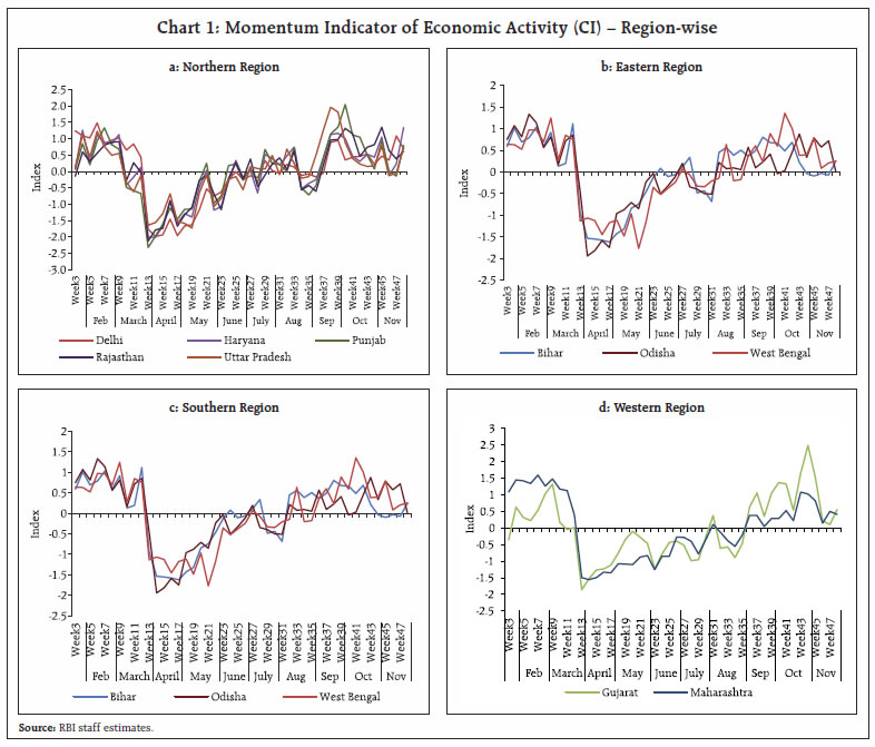 Southern region, which exhibited first sign of positive momentum in August before some moderation in September, picked up again in October. A temporary dip in the momentum during the second week of November reversed quickly in the second half of the month. Western region states lagging other regions, saw first sign of sustained positive momentum in CIs during September, which continued in October and November. Notably, CIs for states in all regions registered sharp upturn in October. Even though some moderation was recorded in November, momentum remained positive and reversed in second half in most of the states. All-India CI, constructed as a weighted average of state CIs by using the shares of states in overall GVA as weights, captures the collapse in activity in Q1 and subsequent recovery (Chart 2.a). The all-India combined indicator also reflects the gradual opening of the economy as indicated by Oxford Stringency Index and provides a consistent real time assessment of economic activity at the national level. Weekly all-India indicator has shown some moderation in second week of November after peaking in last week of October. Dip in momentum, however, reversed in second half of November despite imposition of new restrictions (reflected by increase in Oxford stringency index) like night curfews by few states. To compare with growth in GDP and industrial output (IIP), we use the 3-variables specification of the CI (due to non-availability of data on Google mobility before 2020) and extend our analysis period backward up to January 2019 (i.e. sample period from January 2019 to November 2020). It is found that CI based on 3-variables specifications also broadly shows similar trends for 2020 (Chart 2b). Furthermore, both the 3-variables and 4-variables indicators exhibit co-movement with IIP growth. V. Relationship with Macroeconomic Variables We further attempt to examine the empirical relationship between CI based on 3-variables and key macroeconomic growth variables to ascertain the utility of CI for public policy purpose. In view of data limitation, we empirically investigate the association of CI with the growth in IIP. As a first step, the association of CI with 12-month percentage change in IIP (y-o-y growth) is measured by computing correlation and it could be seen that there exists high level of correlation between two set of variables over the sample period from January 2019 to September 2020 (Table 3). The Chart 2b also displays a clear relationship between 3-variables CI and y-o-y growth in IIP. Next, after checking the stationarity of the series using Augmented Dickey-Fuller unit root tests, we regress IIP growth on 3-variables CI over the sample period January 2019 to September 2020 with the following specification: Where IIPt is 12-months percentage change in IIP and CIt is the average of all-India CI. The results of the two specifications of the regression are furnished in Table 4 below. The results show positive relationship between IIP growth and 3-variables CI indicator with coefficient significant at 1 per cent level in both specifications. In specification 1, we have used Newey- West estimator that provides Heteroskedasticity and Autocorrelation-Consistent (HAC) Standard Errors. In specification II, a dummy is included to account for sharp negative shock in April 2020 due to nationwide lockdown. Furthermore, the results of both regressions show that CI explains about 87 percent and 93 per cent of variation in IIP growth, respectively (adjusted R2 =0.87 and 0.93). | Table 3: Correlation Matrix | | | IIP Growth (Jan 2019- Sep 2020) | IIP Growth (Jan 2019- Mar 2020) | IIP Growth (Jan 2019- Sep 2020 excluding Apr 2020) | | 3 variables Indicator | 0.93 | 0.79 | 0.92 |
Table 4: OLS Regression
(Dependent Variable – IIP growth) | | | (1) | (2) | | Constant | -4.54*** (1.32#) | -3.81*** (0.93) | | 3 variable Indicator | 28.62*** (4.02#) | 22.59*** (2.39) | | Dummy | | -21.96*** | | Adjusted R2 | 0.87 | 0.93 | Notes: 1. ***, **, & * denote statistical significance at 1 per cent, 5 per cent, & 10 per cent, respectively.
2. Figures in parentheses are standard errors.
# denotes HAC standard errors (Newey-West fixed Bandwidth=3.00) | VI. Conclusion The CIs, constructed based on four daily indicators, captures the real-time momentum in economic activity at sub-national as well as national level during the current pandemic. CI across all regions plunged downward sharply following the lockdown in the last week of March, reflecting sharp fall in the economic activity. CI momentum shows that different regions have observed a varying pace of recovery with the gradual unlocking of the economy from June 2020. Each region has experienced intermittent ups and downs depending upon relaxation and tightening of restrictions necessitated by the evolving COVID-19 infections. The Northern region led the recovery in July and August followed by some signs of momentum in Southern and Eastern states. Western region remained behind other regions in the recovery curve but has shown positive momentum September onwards. Overall, all-India CI shows continued sequential improvement in September and October suggesting signs of robust recovery. Despite moderation in November, momentum of economic activity reversed in second half and remained positive. Furthermore, CI has robust positive and statistically significant relationship with growth in industrial output. Since the constructed CI is providing a real-time assessment of economic activity both at the national and sub-national levels, it could provide greater insights for the real-time policy making. References Chetty, R., Friedman, John N., Hendren, N., Stepner, M. and Team (2020), “How Did COVID-19 and Stabilization Policies Affect Spending and Employment? A New Real-Time Economic Tracker Based on Private Sector Data”, Working Paper 27431, National Bureau of Economic Research Working Paper series. Crone, T.M. and Alan Clayton Matthews (2005), “Consistent Economic Indexes for the 50 States”, Review of Economics and Statistics, MIT Press. Dziuban, C. D., and Shirkey, E. C. (1974, March 1), “On the Psychometric Assessment of Correlation Matrices”, American Education Research Journal, 2(2), 211-216. https://doi.org/10.3102/00028312011002211 Geweke (1977), “The dynamic factor analysis of economic time-series models”, Latent Variables in Socio-Economic Models (D. Aigner and A. Goldberger, eds.), North-Holland, New York. Kaiser, H. F. (1970), “A second generation little jiffy” Psychometrika, 401-415, https://doi.org/10.1007/BF02291817 Lewis, Daniel J., Karel Mertens James H. Stock and Mihir Trivedi (2020), “Measuring Real Activity Using a Weekly Economic Index”, Federal Reserve Bank of New York Staff Reports, no. 920. Sargent, T., and Sims, C. (1977), “Business cycle modeling without pretending to have too much a priori economic theory”, Working Papers 55, Federal Reserve Bank of Minneapolis. Stock, J. H., and Watson, M. w. (1998), “Business Cycle Fluctuations in US Macroeconomic Time Series”, NBER Working Paper series, https://www.nber.org/papers/w6528.pdf Winter, J., and Dodou, D. (2012), “Factor recovery by principal axis factoring and maximum likelihood factor analysis as a function of factor pattern and sample size”, Journal of Applied Statistics, 39(4), 695- 710. Zoski, K. W., and Jurs, S. (1996), “An Objective Counterpart to the Visual Scree Test for Factor Analysis: The Standard Error Scree”, Educational and Psychological Measurement, 56(3), 443-451, https://doi.org/10.1177/0013164496056003006.
Annexure 1
* This article has been prepared by Sarthak Gulati, Bipul Kumar Ghosh,and Sunil Kumar from the Monetary Policy Department (MPD). The authorsare thankful to Dr. Rajiv Ranjan and Muneesh Kapur for their valuablecomments on the draft. Views expressed in the article are those of theauthors and do not represent views of the RBI. 1 Coincident Index and Indicator are used interchangeably in this article. 2 https://www.philadelphiafed.org/research-and-data/regional-economy/indexes/coincident 3 https://www.newyorkfed.org/research/policy/weekly-economic-index#/ 4 Data for some states is not available on Vahan platform while a few states have no cities in the daily AQI bulletin released by CPCB. The (x) sign is used denote such unavailability of data. For 2019, due to unavailability of google mobility data, 3-variable indicator is constructed later in the article. |