Inflationary pressures emanating from volatile international crude oil prices, and currency depreciation in the first half of the year, cooled down markedly in the second half, driven down by moderation in crude oil prices and a collapse in food prices. The monetary policy committee cut the policy repo rate by 75 basis points during February-June 2019. Forex operations by the Reserve Bank and large currency expansion exacerbated the pressure on system level liquidity, warranting active liquidity management. Banks’ deposit and lending rates reflected the movements in the policy repo rate, though transmission remained uneven across sectors.

III.1 The conduct of monetary policy in 2018-19 was guided by the objective of achieving the medium-term target for consumer price index (CPI) inflation of 4 per cent with a tolerance band of +/- 2 per cent, while supporting growth. Inflationary pressures emanating from volatile international crude oil prices, and currency depreciation in the first half of the year, cooled down markedly in the second half, driven down by moderation in crude oil prices and a collapse in food prices. CPI inflation averaged 3.4 per cent in 2018-19; 4.3 per cent in the first half and 2.5 per cent in the second half. These diverse movements were reflected in the voting pattern of the monetary policy committee (MPC).

III.2 Forex operations by the Reserve Bank and large currency expansion exacerbated the pressure on system level liquidity during 2018-19, warranting active liquidity management through a variety of instruments: regular repos and reverse repos under the liquidity adjustment facility (LAF); fine-tuning variable rate auctions of both repos and reverse repos; outright open market operations (OMOs); and foreign exchange swaps. Banks’ deposit and lending rates reflected the movements in the policy repo rate during the year, though transmission remained uneven across sectors, reflecting varied credit demand conditions and credit risk.

III.3 Against the above backdrop, section 2 presents implementation status of the agenda set for 2018-19 while priorities of the Monetary Policy Department in 2019-20 have been discussed in section 3.

2. Agenda for 2018-19: Implementation Status

Monetary Policy

III.4 In the first bi-monthly monetary policy statement for 2018-19 (April 5, 2018), the MPC kept the policy repo rate under the LAF unchanged at 6.0 per cent, with five members voting in favour of the decision and one member voting to increase the repo rate by 25 basis points (bps). The stance of monetary policy was retained as neutral. Headline CPI inflation was projected at 4.7-5.1 per cent in H1:2018-19 and 4.4 per cent in H2, with risks tilted to the upside. The decision to keep the policy rate on hold was shaped by several uncertainties surrounding the inflation trajectory such as the revised formula for minimum support prices (MSP) for kharif crops, the risks from fiscal deviations at centre and states’ levels, rising input and output price pressures, and volatility in crude prices. The MPC indicated that it would look through the statistical impact of revisions in house rent allowances (HRAs), while remaining watchful about any second-round effects.

III.5 By the second bi-monthly statement of the MPC in June 2018, inflation had edged up, driven by an abrupt acceleration in inflation excluding food and fuel, even as vegetable prices turned out to be weaker than the usual summers’ upturn. A major upside risk to the baseline inflation path cited in the April resolution - higher crude oil prices - had, however, materialised. These developments, together with rise in other global commodity prices and input cost pressures, led to an upward revision in the CPI inflation projection to 4.7 per cent in H2:2018-19. Developments in global financial markets, a significant rise in household inflation expectations and the uncertainty about the impact of the revisions in the MSP formula for kharif crops were seen as key upside risks. Taking these into consideration, the MPC unanimously voted to increase the policy repo rate by 25 bps but retained a neutral stance. The MPC also noted that there had been a sustained revival in domestic economic activity, and that the output gap had nearly closed.

III.6 In the run-up to the third bi-monthly statement in August 2018, actual inflation outcomes in May and June 2018 turned out to be a little below the trajectory projected earlier, as the seasonal summer surge in vegetables prices remained muted and fruits prices declined. The inflation projection for Q2:2018-19 was revised marginally downwards to 4.6 per cent, marginally upwards to 4.8 per cent for H2:2018-19; and at 5.0 per cent in Q1:2019-20. Volatile crude oil and financial asset prices and hardening of input price pressure in the manufacturing sector were seen as risks to the baseline inflation path besides those cited in June. Against this backdrop, the MPC decided to increase the policy repo rate by 25 bps with five members voting in favour of the resolution and one member voting for a pause.

III.7 By the time of the fourth bi-monthly policy for 2018-19 in October 2018, CPI headline inflation fell from 4.9 per cent in June to 3.7 per cent in August, dragged down by a sharp decline in food inflation. Inflation projections were revised downwards to 3.9-4.5 per cent in H2:2018-19 and 4.8 per cent in Q1:2019-20, with risks somewhat to the upside. However, the inflation outlook was clouded by several uncertainties such as still elevated and volatile international crude oil prices and the risk of higher pass-through from the sharp rise in input prices to retail prices. Against this backdrop, the MPC decided to keep the policy repo rate unchanged but changed the stance to calibrated tightening. Five members voted in favour of keeping the policy rate unchanged and one member voted for an increase in the policy rate by 25 bps. Furthermore, five members voted in favour of changing the stance to calibrated tightening and one member voted to continue with a neutral stance.

III.8 In the run-up to the fifth bi-monthly monetary policy statement of December 2018, inflation eased more than anticipated in September-October 2018, primarily due to the unexpected slipping of food prices into deflation in October, even as inflation in non-food prices registered a broad-based increase. International crude prices fell sharply in November 2018. Accordingly, inflation projections were revised downwards to 2.7-3.2 per cent for H2:2018-19 and to 3.8-4.2 per cent for H1:2019-20, but with risks tilted to the upside. The inflation outlook remained clouded by several factors referred to earlier, apart from the risk of a sudden reversal in prices of perishable food items, volatile financial markets, and elevated households’ inflation expectations. Inflation excluding food remained sticky and elevated. Considering these dynamics, the MPC decided to keep the policy repo rate on hold and maintain the stance of calibrated tightening. While the decision to keep the policy rate unchanged was unanimous, one member voted to change the stance to neutral.

III.9 By the time the MPC met for the sixth bi-monthly policy in February 2019, food prices sank further into deflation for the third consecutive month in December 2018, inflation in the fuel group moderated considerably and inflation excluding food and fuel eased. Inflation projections were revised downwards to 2.8 per cent for Q4:2018-19, 3.2-3.4 per cent for H1:2019-20 and 3.9 per cent for Q3:2019-20 with risks broadly balanced around the central trajectory. On the growth front, keeping in mind the tentative pick-up in domestic credit, the uncertainties on global demand and the likely headwinds for domestic growth, GDP growth for 2019-20 was projected at 7.4 per cent – in the range of 7.2-7.4 per cent in H1, and 7.5 per cent in Q3 – with risks evenly balanced. The output gap had opened up again modestly. Against this backdrop, the MPC reduced the policy repo rate by 25 bps to 6.25 per cent by a majority of 4-2 votes, with two members voting to keep the repo rate unchanged. All the members, however, voted to change the stance from calibrated tightening to neutral.

III.10 The first bi-monthly monetary policy statement for 2019-20 in April 2019 took place in an environment of a slowing down of the growth momentum across advanced economies (AEs) and emerging market economies (EMEs). On the domestic front, food inflation remained in deflation for the fifth consecutive month in February 2019 and the fall in fuel inflation deepened. CPI inflation excluding food and fuel remained below the December print. Taking these developments, and assuming a normal monsoon in 2019, the path of inflation was revised downwards to 2.4 per cent in Q4:2018-19, 2.9-3.0 per cent in H1:2019-20 and 3.5-3.8 per cent in H2:2019-20, with risks broadly balanced. Several factors, however, imparted uncertainties to the inflation outlook: early reports of some probability of El Nino; the risk of an abrupt reversal in food prices; the risk of sustainability of soft fuel inflation; the hazy outlook for crude oil prices; and volatility in financial markets. The MPC noted that the output gap remained negative and the domestic economy was facing headwinds, especially on the global front. Against this backdrop, the MPC decided by a vote of 4-2 to reduce the policy rate by 25 bps to 6.0 per cent, with two members voting for a pause. The MPC maintained the neutral stance of monetary policy by a majority of 5-1, with one MPC member voting in favour of changing the stance to accommodation.

III.11 In the second bi-monthly monetary policy meeting of June 2019, the MPC unanimously decided to reduce the policy repo rate by 25 bps to 5.75 per cent and change the stance of monetary policy from neutral to accommodative. This decision was based on an assessment of a weakening of growth impulses since the April 2019 policy, driven by a sharp slowdown in investment activity along with continuing moderation in private consumption growth, and a widening of the output gap. Headline inflation was projected at 3.0-3.1 per cent for H1:2019-20 and 3.4-3.7 per cent for H2, remaining below the target, even after considering the expected transmission of the past two policy rate cuts. Given this scenario, the MPC saw scope to ease policy rate further to boost aggregate demand while remaining consistent with its flexible inflation targeting mandate.

III.12 The output gap – the deviation of the actual output level from its potential level – is a proxy for demand-supply mismatches and plays an important role in medium-term inflation dynamics. Recent research has highlighted that a macro-financial model allowing for inter-linkages between economic and financial cycles could provide a more comprehensive view of demand conditions, potential output and natural rate of interest (Box III.1).

Box III.1 Interlinkage between Financial and Economic Cycles There is a growing body of literature which suggests that the estimation of economic cycle/output gap can be substantially improved by including information on the financial cycle, especially during boom/bust phases. A macro-financial model estimated by augmenting the Monetary Policy Model (MPMOD)1 (Alichi et al., 2018), with a financial block (Juselius et al., 2017), helps to understand the interlinkage between financial and economic cycles in India (Chart 1). In this framework, the financial cycle - measured by two indicators viz., the leverage gap and the debt service gap2 - impacts real economic activity with a lag. The interest rate feeds into the leverage gap - firming up of the real interest rate gap brings down asset prices. The debt service gap depends on the long-term interest rate - an increase in the nominal lending rate increases the interest payment burden and, in turn, the debt service gap. The leverage and debt service gaps have bi-directional linkages running from new debt to debt service to asset prices and then back to the leverage gap. The debt service gap feeds negatively into asset price growth and, hence, boosts the leverage gap. Apart from cyclical variables, long-term trend variables are also interlinked in the model. The natural rate of interest (r*) is related positively to the growth rate of potential output. 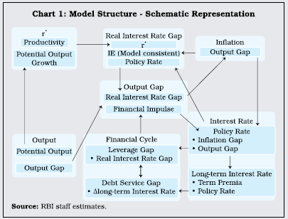Quarterly data from Q2:2008-09 to Q2:2018-19 are used for the exercise, and the system of equations is estimated in a Bayesian framework. The empirical estimates suggest that (i) an increase in the debt burden has a negative impact on asset price growth, pushing up the leverage gap, tightening financial conditions and the output gap (Chart 2a), which leads to reduction in interest rates and brings the debt burden back to steady state; (ii) an increase in leverage leads to decline in credit expansion and a fall in the credit-GDP ratio, which tightens financial conditions and leads to a fall in the output gap (Chart 2b); and (iii) an increase in the policy interest rate increases long-term interest rates with some negative impact on asset prices; the resulting tightening of financial conditions lead to the widening of a negative output gap (Chart 2c). A comparison of the output gap estimates filtered out from the macro-financial model vis-à-vis the MPMOD indicates that during 2012 to 2017, high non-performing asset ratios, coupled with a sharp fall in credit growth contributed to tighter financial conditions, which in turn strained demand conditions (Chart 3). Subsequently, as the impact of this configuration diminished over time, it spurred some recovery in credit markets and a revival in asset markets, leading to a faster closing of the output gap from 2017. 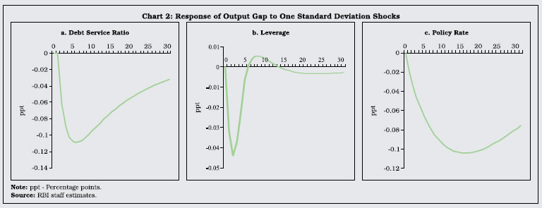During 2012 to 2017, the output gap estimates obtained by incorporating the financial cycle were lower than estimates without it. Thus, with a given level of the overall output, estimates of the potential output are found to be higher than the ones estimated without the financial information. Consequently, the estimates of the natural rate of interest were also higher during that period. On the other hand, the output gap estimates were found to be higher since 2017; the potential output and natural rate of interest were lower in comparison with the estimates without including the financial cycles. References: 1. Alichi, A., Al-Mashat, R. A., Avetisyan, H., Benes, J., Bizimana, O., Butavyan, A., and Others (2018). ‘Estimates of Potential Output and the Neutral Rate for the US Economy’, International Monetary Fund Working Paper No. WP/18/152. 2. Juselius, M., Borio, C., Disyatat, P., & Drehmann, M. (2017). ‘Monetary Policy, the Financial Cycle, and Ultra-Low Interest Rates’, International Journal of Central Banking, 13(3), 55-89. 3. Rath, D. P., Mitra, P., & John, J. (2019). ‘Interlinkage between Financial and Economic Cycles - Some Evidence using a Macro-Financial Model for India’, Mimeo.

The Operating Framework: Liquidity Management

III.13 The operating framework of monetary policy aims at aligning the operating target – the weighted average call rate (WACR) – with the policy repo rate through proactive liquidity management, consistent with the stance of monetary policy. During 2018-19, the Reserve Bank applied multiple tools to manage both frictional and durable liquidity. While liquidity amounting to ₹6.4 trillion was injected through variable rate repos of maturities ranging from overnight to 56 days in addition to the regular 14-day repos, liquidity of ₹42.8 trillion was absorbed through reverse repos of maturities ranging from overnight to 14 days. The Reserve Bank also conducted 27 open market purchase operations aggregating about ₹3.0 trillion during the year. Based on an assessment of financial market conditions, the Reserve Bank increased the Facility to Avail Liquidity for Liquidity Coverage Ratio (FALLCR)³ twice in 2018-19 by 2 percentage points of NDTL on each occasion, to reach a total of 13 per cent of NDTL, which supplemented the ability of individual banks to avail liquidity from the repo market against high-quality collateral. Furthermore, it was decided to reduce the statutory liquidity ratio (SLR) by 25 bps every calendar quarter beginning January 2019, until it reached 18 per cent of NDTL, in order to align the SLR with the liquidity coverage ratio (LCR) requirement. To further harmonise the liquidity requirements of banks with the LCR, a roadmap was given in April 2019 to increase the FALLCR by 50 bps in four steps to reach 15 per cent of NDTL by April 2020.

Drivers and Management of Liquidity

III.14 Reflecting domestic and global financial market conditions, systemic liquidity underwent significant shifts during 2018-19. Capital outflows triggered by global trade tensions and faster than anticipated normalisation of the US monetary policy exerted downward pressure on the domestic currency. Consequently, forex operations by the Reserve Bank sucked out domestic liquidity. Large currency expansion was another feature throughout the year, exacerbating the pressure on system level liquidity.

III.15 In Q1:2018-19, liquidity conditions generally remained in surplus in the wake of large government spending. The resulting flow of liquidity into the system (₹1.4 trillion in April) more than offset the liquidity drained by two autonomous factors – currency expansion by ₹743 billion and forex sales of ₹160 billion – during the month (Chart III.1). The scale of forex sales picked up in May and June, and higher than usual currency expansion continued, resulting in a liquidity deficit in the system for a brief period from mid-June to July 2018, further exacerbated by advance tax outflows. Accordingly, in addition to the regular 14-day repos, the Reserve Bank injected liquidity through overnight variable rate repos on a few occasions to tide over the transitory liquidity tightness. In addition, the Reserve Bank also conducted OMO purchases of ₹100 billion each in May and June 2018 to infuse durable liquidity into the system. Overall, net liquidity absorption under the LAF moderated progressively during the quarter from an average daily net position of ₹496 billion in April to ₹140 billion in June.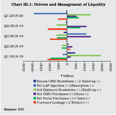

III.16 During Q2:2018-19, liquidity conditions gyrated between deficit and surplus. In July, moderation in government spending (especially in the second half) and the Reserve Bank’s forex sales necessitated average daily net injection of ₹107 billion under the LAF. OMO purchases amounting to ₹100 billion were also conducted during the month. The system moved back into absorption mode in August (up to August 19) due to increased spending by the centre which even warranted recourse to ways and means advances (WMA) from the Reserve Bank, although indirect tax payments whittled down excess liquidity for a brief period. The Reserve Bank absorbed ₹30 billion on an average daily net basis during the month, even as systemic liquidity turned into deficit between August 20 and 30, necessitating liquidity injection. The system moved back into surplus during August 31 - September 10, as government spending increased in the first half of September; however, system liquidity swung back into deficit due to advance tax outflows. The Reserve Bank undertook daily net injection of liquidity through the LAF of ₹406 billion along with two OMO purchases amounting to ₹200 billion in the second half of September to meet durable liquidity requirements (Chart III.2).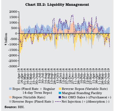

III.17 Liquidity conditions generally remained in deficit during Q3:2018-19. A combination of increased festival related currency demand and the Reserve Bank’s forex sales resulted in a deficit in the second week of October 2019, which continued for the rest of the month. With the centre resorting to WMA, the deficit moderated at the beginning of November, but increased subsequently as currency expansion was sustained during the festival season. The deficit increased further in the second half of December, mainly on the back of advance tax outflows. The Reserve Bank conducted variable rate repo auctions of various tenors, including longer term (28 days and 56 days) in addition to regular 14-day term repos. Additionally, durable liquidity of ₹360 billion was injected through OMOs in October, which was subsequently scaled up to ₹500 billion each in November and December, taking the total durable liquidity injection through OMOs to about ₹1.4 trillion during the quarter (Chart III.3). Variable rate reverse repo auctions were conducted to mop up excess liquidity.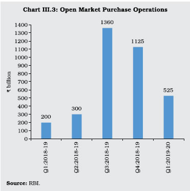

III.18 Deficit liquidity conditions persisted in Q4:2018-19 in the wake of sustained currency expansion and build-up of government cash balances, barring a few days at the beginning of both January and February, when liquidity conditions turned surplus as the government resorted to overdraft (OD)/WMA. In order to meet durable liquidity needs, the Reserve Bank conducted OMO purchases of ₹500 billion in January, ₹375 billion in February and ₹250 billion in March. Simultaneously, transient liquidity needs were met through variable rate repos of various tenors in addition to the regular 14-day term repos.

III.19 With the Reserve Bank meeting durable liquidity needs on a regular basis through OMOs, LAF positions on most occasions reflected movements in government spending (Chart III.4).

III.20 To sum up, the Reserve Bank’s forex operations and currency expansion were the primary drivers of durable liquidity in the banking system in 2018-19, while government spending was the key driver of frictional liquidity movements. Fine-tuning operations through variable rate auctions were the key instrument through which frictional liquidity was managed. Repo/reverse repo auctions of various maturities were frequently used for managing liquidity (Table III.1).

III.21 In view of increased liquidity demand every year in March due to year-end factors, the Reserve Bank conducted four longer term variable rate repo auctions (tenor ranging between 14-day and 56-day) in March 2019 in addition to the regular 14-day variable rate term repo auctions. Furthermore, the Reserve Bank decided to augment its liquidity management toolkit and injected rupee liquidity for longer duration through long-term foreign exchange buy/sell swaps. Accordingly, it conducted USD/ INR buy/sell swap auction of US$ 5 billion for a tenor of 3 years on March 26, 2019 to inject durable liquidity of ₹345.6 billion.

III.22 After remaining in deficit during April and most of May, systemic liquidity turned into surplus in June driven by large government spending after the general elections. The Reserve Bank absorbed liquidity of ₹517 billion in June, as against an injection of ₹700 billion in April and ₹334 billion in May on a daily net average basis under the LAF. During Q1: 2019-20, the Reserve Bank conducted four OMO purchase auctions – two each in May and June amounting to ₹250 billion and ₹275 billion, respectively. It also conducted a US$ 5 billion buy/sell swap auction amounting to ₹348.7 billion for a tenor of 3 years on April 23 to inject durable liquidity into the system.

Operating Target and Policy Rate

III.23 As alluded to earlier, the objective of liquidity management is to align the WACR – the operating target – with the policy repo rate. During 2018-19, the WACR generally traded below the policy repo rate till January 2019, but hardened intermittently thereafter and spiked at the year-end (Chart III.5). During Q1:2019-20, the WACR showed two-way movements around the policy repo rate.

III.24 The negative spread of the WACR over the repo rate moderated from 11 bps in April to 5 bps in October 2018 but increased thereafter to 12 bps in January (Chart III.6). Post announcement of reduction in the repo rate by 25 bps on February 7, 2019, the WACR broadly aligned with the repo rate in February and March 2019. Overall, the WACR remained 8 bps below the policy rate in 2018-19 (10 bps in H1 and 6 bps in H2). During Q1:2019-20, the WACR averaged close to the repo rate.

Monetary Policy Transmission

III.25 Following the 50 bps increase in the policy repo rate during June-August 2018 (25 bps each in June and August 2018), banks raised their deposit and lending interest rates (Table III.2). Banks had started raising their term deposit rates even earlier - from December 2017 - as surplus liquidity in the system waned. The rise in term deposit rates exerted upward pressure on the cost of funding of banks, which fed into their marginal cost of funds-based lending rates (MCLRs). Consequently, the weighted average lending rate (WALR) on fresh rupee loans sanctioned by banks increased by 57 bps during the tightening phase of the monetary policy cycle (June 2018 – January 2019). The rise in the WALR on outstanding rupee loans was, however, muted (Chart III.7a).

III.26 In response to the reduction in the policy repo rate by 75 bps during February - June 2019, the WALR on fresh rupee loans declined by 29 bps over the same period (Chart III.7b). However, the WALR on outstanding rupee loans increased by 5 bps mainly due to two reasons. First, lending interest rates are typically linked to 1-year MCLR; consequently, interest rates on such loans are reset annually on the due dates. Second, a portion of the loans contracted during July 2010 – March 2016 and still outstanding continues to be linked to the base rate, which remained practically unchanged during both the tightening and easing phases.

Sectoral Lending Rates

III.27 Monetary transmission remained uneven across sectors, reflecting varied credit demand and credit risk. During the tightening phase (June 2018-January 2019), interest rates on outstanding loans increased in respect of sectors such as agriculture, housing and education, while they declined in the case of industry, trade and professional services sectors (Table III.3). During the easing phase beginning from February 2019, lending rates declined for most sectors.

III.28 The Reserve Bank had proposed in December 2018 that all new floating rate personal/retail loans (housing, auto, etc.) and floating rate loans to micro and small enterprises extended by banks beginning April 1, 2019 would be benchmarked to external benchmarks, viz., (i) the policy repo rate; or (ii) any benchmark market interest rate produced by the Financial Benchmarks India Private Ltd. (FBIL), including Treasury bill rates. Taking into account the feedback received during discussions held with stakeholders on issues such as (i) management of interest rate risk by banks from fixed interest rate linked liabilities against floating interest rate linked assets; and (ii) the lead time required for IT system upgradation, it was decided in April 2019 to hold further consultations with stakeholders and work out an effective mechanism for transmission of rates.

III.29 During 2018-19, studies were undertaken on a range of issues to improve the analytical inputs for the conduct of monetary policy: an examination of drivers of the investment cycle to understand the duration of investment cycles and inflexion points/structural breaks; determinants of economic activity, and the role of monetary and fiscal policies; the incorporation of a fiscal block in the quarterly projection model for an enhanced understanding of monetary-fiscal interface; estimates of the finance-neutral output gap which incorporates the role of financial factors (bank credit, equity prices and policy repo rate) in assessing demand conditions; an assessment of the impact of minimum support prices and house rent allowances on inflation; macroeconomics of crude oil prices; and, forex market operations and liquidity management. Research studies were also undertaken on measurement issues relating to housing services in CPI and the role of monetary policy in movement of bond yields.

3. Agenda for 2019-20

III.30 During 2019-20, the focus will be on refining the liquidity forecasting framework, sharpening the estimation of currency in circulation at various frequencies (such as yearly, quarterly, monthly, fortnightly and weekly) and an overall reviewing of operational aspects of the liquidity management framework, including aspects relating to structural liquidity balance and distributional asymmetry in liquidity.

III.31 An analysis of recent food inflation dynamics will be carried out to understand the sources of volatility and to examine the relative role of cyclical and structural factors at play. Furthermore, the nature of spatial dimensions of inflation will be studied to better understand the divergences in inflation rates across major groups/sub-groups and changes in them over time. In order to enhance the understanding of monetary transmission, an analysis of sectoral credit flows would be undertaken. The implications of the asset quality/health of the banking sector and NBFCs on credit flows to the commercial sector would also be examined.

¹ MPMOD applies the multivariate filter methodology to estimate the output gap and potential output.

² The characterisation of the financial cycle is based on two long run relationships that together determine the long run sustainability of the credit-GDP ratio. The first relationship is between the credit-GDP ratio and real asset prices, which is a proxy for collateral constraints. The deviation of this relationship from its long-term trend is defined as the leverage gap. The second relationship is between the credit-GDP ratio and the nominal lending rate, which captures the effect of cash flow constraints due to interest payments faced by the households. The deviation of this relationship from its long-term trend is defined as debt service gap (Juselius et al., 2017).

³ The assets allowed as Level 1 High Quality Liquid Assets (HQLAs) for the purpose of computing LCR of banks include, inter alia, government securities in excess of the minimum SLR requirement and, within the mandatory SLR requirement, government securities to the extent allowed by the Reserve Bank under Marginal Standing Facility (MSF) [presently 2 per cent of the bank’s NDTL] and under the FALLCR.