by Bipul Ghosh^, Narendra Singh#, Sandhya Kuruganti* The delayed availability of official state-level Gross State Value Added (GSVA) data creates significant limitations for high-frequency measurement and real-time assessment of subnational economic activity in India. This study presents a novel and scalable framework for quarterly growth estimation aimed at addressing data gaps and reducing data lags by integrating satellite-based night-time lights with behavioural indicators from Google Trends, with empirical application to Gujarat, Maharashtra, and Karnataka. Year-on-year changes in satellite-based light intensity are used to track short-term movements in economic activity. The framework combines geospatial and behavioural signals within a statistical modelling approach, improving the accuracy of short-term growth estimates and enabling the construction of high-frequency proxy indicators that can supplement official state-level statistics during the period before quarterly estimates become available. Introduction Evidence-based economic analysis requires timely and granular data for accurate measurement, particularly in a geographically and structurally diverse country like India. Although national-level Gross Domestic Product (GDP) statistics have been released quarterly since 1996-97, state-level estimates of Gross State Value Added (GSVA) are available only annually and with considerable lag. The typical lag of 12 to 18 months creates significant constraints in capturing evolving regional economic dynamics in real time. Given the significant heterogeneity in economic structures, sectoral compositions, and growth drivers across Indian states, there is a pressing need for tools that can generate more frequent, high-resolution economic indicators at the subnational level. Recent developments in alternative data sources and computational methods offer a possible pathway to address this data availability and frequency gap. High-frequency and publicly accessible datasets such as satellite-based night-time lights (NTL) and digital behavioural indicators from Google Trends (GT) have emerged as valuable proxies for high-frequency estimation of economic activity. Although prior studies have used NTL and GT data independently in various empirical applications, their combined use remains unexplored. This article develops the idea that integrating spatial signals from NTL with behavioural insights from GT can offer a more comprehensive and complementary picture of regional economic dynamics, capturing both infrastructure-linked production capacity and shifts in consumer sentiment or labour market activity. There are two main sources of satellite-based NTL data: the Defense Meteorological Satellite Program’s Operational Linescan System (DMSP/OLS), which offers annual data from 1992 to 2013, and the more recent Visible Infrared Imaging Radiometer Suite (VIIRS), operational since 2011. VIIRS provides substantially higher spatial and radiometric resolution along with improved calibration procedures. It is the basis for NASA’s Black Marble product suite, which is used in this study. Google Trends, on the other hand, offers a high-frequency lens into population level search behaviour. By capturing the intensity of interest in economic topics such as jobs, consumption goods, credit, and housing, GT provides an indirect but timely measure of economic sentiment and behavioural shifts. Although several studies have leveraged Google Trends to estimate or forecast national level economic indicators, its integration with spatial luminosity data for subnational nowcasting remains rare. This article presents a novel and scalable framework to estimate quarterly GSVA growth for three economically significant Indian states, Gujarat, Maharashtra, and Karnataka, by combining two high frequency and open-access proxies: satellite-based NTL data from NASA’s Black Marble dataset and behavioural indicators from Google Trends. To the best of our knowledge, this is the first attempt in the Indian context to (i) estimate quarterly state-level economic activity using calibrated night-time light intensity and (ii) integrate these estimates with real-time digital behavioural data within a unified modelling framework. The study offers a substantial contribution to addressing gaps in high-frequency subnational economic measurement. Given the increasing need for timely and granular information, tools for high frequency regional economic estimation can provide a useful supplement to official statistics. Such tools not only enhance the availability of real-time economic indicators but also facilitate better coordination between central and state governments in the pursuit of inclusive and balanced growth. The rest of the paper is structured as follows: Section II reviews the existing literature and presents the study area. Section III details the datasets used, including NTL, Google Trends, and GSVA statistics. Section IV explains the methodological framework. Section V presents and discusses the results. Section VI concludes with the study’s main findings and outlines avenues for future research. II. Literature Review In economic research, the appeal of NTL data lies in its free access, global scope, and high frequency. It is widely used to complement or substitute traditional economic indicators, especially where data quality is poor. Chen and Nordhaus (2011) found NTL useful in assessing the reliability of national statistics, particularly in low-capacity countries. NTL data’s fine spatial resolution enables subnational economic analysis. Henderson et al. (2012) introduced the concept of inverse elasticity between NTL and GDP using DMSP-OLS data, further applying their model to sub-Saharan Africa. This approach quantified how changes in GDP are reflected in NTL brightness, making it a useful proxy in countries with scarce economic data. Later works expanded on this. Keola et al. (2015) integrated land cover data to enhance GDP estimates over developing countries, but their performance worsened in economies with high diversity due to the limits of general land cover classification. Similarly, Hu and Yao (2018) noted poorer estimates of GDP per capita over low- and middle-income countries and stressed the value of NTL in such contexts. Beyer et al. (2018) estimated NTL-GDP elasticity for South Asia using both DMSP-OLS and VIIRS data. Their findings indicated that there was consistency in the relationship between GDP and NTL for countries such as India and Nepal, with robust state-level estimates within India, but decreased accuracy in places like Maldives. They stressed the need for improvement in data cleaning to enhance estimation accuracy. Prakash et al. (2019) continued this work, using cleaned VIIRS data and quarterly GDP over India. They found high elasticity between NTL and GSDP, though combining DMSP-OLS and VIIRS over long periods showed calibration errors. Hence, they recommended the use of consistent VIIRS datasets while performing long-term studies. Bhadury et al. (2018) employed cleaned VIIRS data and other high frequency inputs in a nowcasting model. The study demonstrated that NTL improves accuracy, especially for India’s trade and service sectors. Similarly, NTL data were used to track the economic impacts of COVID-19 in India (Ghosh et al. 2020 and Dasgupta 2022). Beyer et al. (2022) found that the NTL-GDP correlation was stronger in emerging economies than in developed ones, reinforcing NTL’s role in low data environments. However, using NTL as an economic proxy has challenges. Nordhaus and Chen (2015) showed that mismatches in the spatial resolution of NTL data and administrative boundaries make it hard to integrate this information with official economic statistics. Despite these problems, investigators continued to enhance methods by improving preprocessing, merging NTL with auxiliary datasets, and focusing on higher quality VIIRS imagery. These efforts refine the precision and suitability of NTL data in economic and policy research. Along with the NTL data, GT has emerged as a high frequency data source for tracking economic activity. GT tracks changes in public interest in real time through their search behaviour and can inform about consumer sentiment, unemployment trends, and spending intentions. Woloszko (2020) developed the OECD Weekly Tracker using GT data and neural network-based models to estimate real time GDP growth for 46 OECD and G20 countries, particularly during crises such as COVID-19. This shows the rising potential of non-traditional data, including both NTL and GT, as these can complement traditional statistics with granular and timely economic indicators. Past research has pointed out that NTL data tends to be more responsive, yielding more accurate results in urban and industrial areas rather than in low-density rural regions. These studies warn that in rural areas, where economic activities are dispersed and not as intense, this may not be a consistently reliable proxy. To address this, the present study selected three states (Gujarat, Maharashtra and Karnataka) that are among the top industrial states in India, according to the Annual Survey of Industries report 2022-23. Among these, Karnataka was chosen over Tamil Nadu and Andhra Pradesh due to its higher number of high quality pixels in the monthly NTL images, which facilitated more precise analysis during the study. III. Datasets Satellite Data For this study, the Black Marble Night-time Lights (NTL) monthly product (VNP46A3) corrected for moonlight and atmosphere was utilised. This product has a spatial resolution of 15 arc-seconds (~0.5 km) and is available from the LAADS DAAC website1 starting from January 2012 (Table 1). The study collected VNP46A3 data from April 2012 to December 2024 for the study area. The VNP46A3 product is provided in the standard land Hierarchical Data Format Earth Observing System (HDF-EOS) format (i.e., HDF5 format). The product has 28 layers containing data on NTL Radiance Images, the number of observations, quality layers, and standard deviation measures for multi-view zenith angle categories (near-nadir, off-nadir, and all angles), snow status (snow-covered and snow-free), as well as a land-water mask, platform, latitude, and longitude. For more detailed information about the VNP46A3 product, refer to the Black Marble User Guide (Version 1.3). | Table 1: Details of Satellite-based Night-time Light (NTL) Data | | Satellite and Sensor | SNPP and VIIRS | | Product Name and file Format | Black Marble NTL product (VNP46A3) in HDF5 format | | No of Layers in VNP46A3 HDF5 | 28 | | Name of Image/Layer used | All Angle Composite Snow Free and Quality | | Spatial Resolution | 15 arc-seconds (~500 meter) | | Temporal Resolution | Monthly | Google Trends Data In the present study, monthly Google Trends data for 25 categories were utilised for the states of Maharashtra, Karnataka, and Gujarat covering the period from 2010 to December 2024 (Table 2). These categories were selected to capture a wide range of economic and social behaviours relevant to state-level economic activity. The data were obtained from the official Google Trends website, which offers open access to normalised search volume indices, enabling researchers to explore real-time public interest and behavioural trends over time2. Gross State Value Added Data Gross State Value Added (GSVA) data were sourced from the Ministry of Statistics and Programme Implementation (MOSPI). From GSVA, a modified version is derived called ‘Modified GSVA’, which excludes low illumination sectors such as agriculture, forestry, fishing, mining, public administration and others. This adjustment aims to better align economic activity with NTL emissions, based on the assumption that certain sectors such as industry, trade, construction, and related services contribute more significantly to observed radiance. | Table 2: List of 25 Google Trends Categories | | Travel | Law & Government | Internet & Telecom | | Sports | People & Society | News | | Real Estate | Computer & Electronics | Online communities | | Jobs and Education | Finance | Pets & Animals | | Shopping | Hobbies & Leisure | Food & Drink | | Beauty & Fitness | Science | Health | | Autos & Vehicles | Art & Entertainments | Games | | Homes & Garden | Books & Literature | | | Business & Industrial | Reference | | IV. Methodology Satellite-based Night-time Light (NTL) Data Processing The present study processes monthly NASA Black Marble remote sensing HDF5 product to compute the sum of light (SOL) within the study area for each financial quarter during the period from April 2012 to December 2024. Among the three available view angle categories (all-angle, near-nadir, and off-nadir), the study specifically utilises the all-angle, snow-free monthly NTL raw radiance images extracted from the NASA Black Marble HDF5 datasets, as they are more effective at capturing diverse light sources, including direct illumination, reflections from building facades, and indoor lighting visible through windows. To ensure data quality, the corresponding quality flag3 images were extracted for each month. These images, encoded as 8-bit unsigned integers (range: 0–255), were used to identify and exclude low quality pixels. Radiance pixels located at positions flagged as poor quality (value = 1 in the quality image) were excluded from analysis. The resulting filtered, snow-free radiance images, stored as 16-bit unsigned integers (range: 0–65535), were exported in Geographic Tagged Image File Format (GeoTIFF) for further processing. Chart 1 shows the all-angle composite snow-free image, the quality image, and the all-angle composite snow-free radiance image after poor pixel removal. Subsequently, all good-quality images of a particular month covering the study area were mosaicked. In the final step, the mosaic images were converted to physical radiance units by applying a scale factor of 0.1 and reprojected to the world geographic coordinate system -1984. This process was repeated for each month from April 2012 to December 2024. The quarterly composite NTL images were generated by calculating the median of monthly radiance images for each 3-month period in the financial year. The median was chosen over the mean because it discards low and high radiance outliers. This study selected three industrial states — Gujarat, Maharashtra, and Karnataka as the study area. 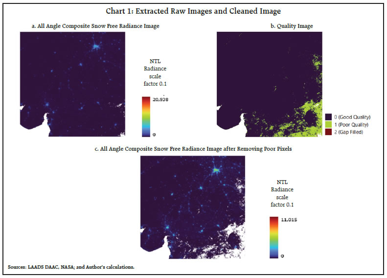 The radiance image for each quarter was spatially subset to state boundaries in Quantum Geographic Information System (QGIS). Because of low detection limits on moonless nights, the NTL usually contains significant background noise4 that must be filtered for an accurate analysis of human-induced lighting. To eliminate this, several sample areas outside human settlements, devoid of artificial light sources, were randomly selected within the study region using high resolution imagery from Google Earth Pro. The average radiance of these sample areas was analysed and used as a threshold for filtering out background noise. After background noise removal, the total NTL radiance for each financial quarter was calculated for Gujarat, Maharashtra, and Karnataka. All geospatial processing and radiance calculations were carried out using QGIS software5. Year-on-year (y-o-y) growth for each quarter was then computed by comparing the radiance value of a given quarter with the corresponding quarter from the previous year. Correlation analysis between the quarterly growth of SOL radiance and GSVA for each state was conducted and evaluated. Google Trends Data Processing Google Trends data also required careful handling. The sampling noise and discontinuities due to change in Google’s methodology (especially in January 2011 and January 2016) were present in raw Search Volume Index (SVI). Therefore, SVI for each category was downloaded five times at 15-minute intervals and averaged to reduce sampling variability. Subsequently, log transformation was applied to stabilise variance and structural breaks were corrected by adjusting series around breakpoints to ensure continuity. Monthly SVIs were averaged into quarterly values, and y-o-y growth rates were computed using first differences over four quarters. Only those categories that had statistically significant correlation with GSVA were kept. Dimensionality was further reduced using Principal Component Analysis (PCA), and the top components were used in the empirical model. GSVA Data Processing GSVA constitutes the subnational analogue of GDP in the Indian system of national accounts and is published at an annual frequency. To recover intra-year dynamics required for empirical analysis, annual GSVA series are temporally disaggregated to the quarterly frequency using the Denton proportional benchmarking method (1971), which represents the standard approach for reconciling low frequency benchmarks with high frequency indicators in national accounting practice (IMF, 2017). The Denton procedure preserves the short-run movements of the indicator series while imposing exact consistency with annual totals, thereby minimising measurement-induced volatility and ensuring coherence between short- and long-run dynamics. This approach is consistent with India’s official statistical methodology, where benchmark indicator techniques underpin the construction of quarterly GDP estimates. Quarterly GSVA estimates are obtained by mapping the national quarterly GDP seasonal profile onto state level annual GSVA data. This assumption is particularly appropriate for large industrialised states such as Maharashtra, Gujarat, and Karnataka, which together account for roughly 30 per cent of aggregate output and play a central role in shaping national business cyclical and seasonal movements. The national seasonal pattern is therefore an aggregation of state-level dynamics rather than an externally imposed construct. These states are exposed to common macroeconomic drivers, including monsoon-related seasonality, similar fiscal cycles, and synchronised industrial production patterns. Under these conditions, the imposed seasonal structure provides a reasonable approximation of intra-year state level fluctuations while preserving consistency with the national accounts. ARIMAX Model This study employs an Auto-Regressive Integrated Moving Average model with eXogenous inputs (ARIMAX) to estimate quarterly GSVA growth using contemporaneous external indicators. The ARIMAX model extends the classical ARIMA framework by incorporating external regressors alongside lagged values of the dependent variable. In this setup, a pseudo-real-time expanding-window approach is adopted, with GSVA data through quarter t−1 and contemporaneous exogenous indicators for quarter t used to estimate current quarter GSVA growth. The ARIMAX (p, 0, q) model is formulated as: where: p ∈ {0,1,2}, q ∈ {0,1}, d = 0 Yt represents the GSVA growth at time t, Xmt = represent the m-th exogenous regressors at time t, such as night-time light growth and principal components derived from relevant indicators, φi is the autoregressive coefficient, βm = Coefficients associated with the exogenous regressors; θj = moving-average coefficients εt is the error term. Prior to estimation, the stationarity of GSVA growth, NTL growth and the retained Google Trends principal components was examined using Augmented Dickey–Fuller (ADF) and KPSS tests. The results supported stationarity of the variables entering the models across all three states, providing support for the use of d = 0 in the ARIMAX specification. Alternative ARIMAX models were estimated for each state and evaluated using information criteria (AIC and BIC), out-of-sample RMSE and MAE, and residual autocorrelation diagnostics.6 As no single specification performed best across all states and evaluation metrics, the final model was chosen by balancing statistical adequacy, predictive performance, parsimony, and residual diagnostics. Accordingly, ARIMAX(1,0,0) was selected for Maharashtra and Karnataka, while ARIMAX(2,0,0) was selected for Gujarat, where it improved out-of-sample performance and resolved the residual autocorrelation observed under ARIMAX(1,0,0). Details of the model comparison and diagnostic tests are provided in Appendix A3. V. Results and Discussion This study first investigates the relationship between year-on-year (y-o-y) quarterly growth in NTL and the GSVA for three Indian states. Monthly VIIRS DNB NTL time series data, starting from April 2012, were processed to generate quarterly radiance composites for the period 2012–13 up to the third quarter of 2024–25. Subsequently, the total NTL radiance and its year-on-year growth series were computed for each state. In the case of Gujarat, annual GSVA data is available only up to 2023-24, so the analysis of NTL and GSVA was conducted for the period 2012-13 to 2023-24. Chart 2 illustrates the significant expansion in the spatial extent of high NTL radiance values across the observed states during the study period, indicating an increase in night-time light activity over time. The growth per cent of NTL and GSVA has been evaluated for all three states during the observation period. A clear dip in both NTL and GSVA growth was observed during 2020-21Q1 attributed to the impact of COVID-19 (Chart 3). Quarterly night-time lights growth exhibits a strong and statistically significant association with both total GSVA growth and modified GSVA growth across all three states, with correlation coefficients significant at the 5 per cent level (Table 3). This indicates that high frequency variations in NTL closely track underlying state level economic activity as captured by both official and adjusted GSVA measures. To assess robustness, the correlation analysis is repeated after excluding COVID-19 affected quarters from 2019–20Q4 to 2021–22Q2. The estimated relationships remain strong and statistically significant, suggesting that the linkage between NTL growth and GSVA growth is not driven by crisis period anomalies but reflects normal economic dynamics (Chart 3). These results support the use of NTL as a reliable proxy for real-time economic activity outside periods of extreme shocks. 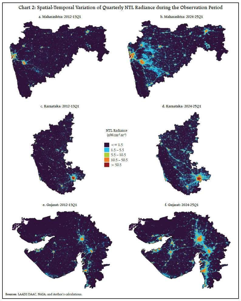
| Table 3: Correlation of y-o-y Quarterly NTL Growth with GSVA Growth and Modified GSVA Growth | | States | Observation Period | Correlation | | | Total GSVA | Modified GSVA | | Maharashtra | 2012-13 to 2024-25 | 0.90 | 0.90 | | Karnataka | 2012-13 to 2024-25 | 0.79 | 0.75 | | Gujarat | 2012-13 to 2023-24 | 0.66 | 0.60 | In addition to quarterly NTL growth, the study also incorporated quarterly GT growth data to improve the estimation of GSVA growth. However, only those GT categories that exhibited a statistically significant correlation with GSVA at the 5 per cent level were selected. The Table A1 presents the correlation coefficients and corresponding p-values, identifying GT categories that have a statistically significant relationship with economic activity, measured through Modified GSVA, in each state. Based on this analysis, Table A2 lists the GT categories selected for further processing through Principal Component Analysis (PCA) for Maharashtra, Karnataka, and Gujarat. A similar procedure was followed for Total GSVA to identify relevant GT categories. Several GT categories met the significance criterion; however, including all of them as external variables would increase model complexity and risk overfitting. To address this, a dimensionality reduction technique, Principal Component Analysis (PCA), was applied to the selected GT categories. The scores of the top principal components were then used as inputs in the ARIMAX specification. For each state, a final selection of principal components was based on minimising the Root Mean Squared Error (RMSE). It was noted that the sports category for Karnataka and Gujarat, though statistically significant, increased RMSE due to its high volatility. Hence, the sports category was excluded from the set of statistically significant GT categories used to generate PCA scores for Gujarat and Karnataka. 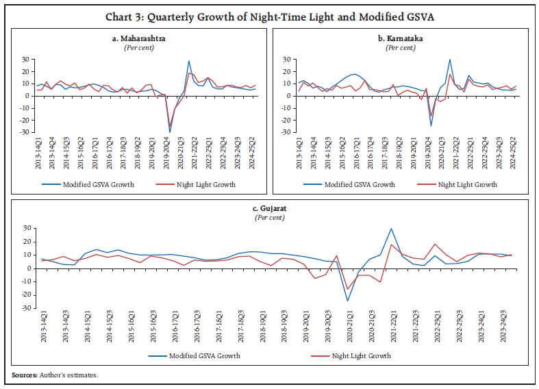 Further, the ARIMAX model was evaluated using an expanding window approach for both total GSVA growth and modified GSVA growth, using NTL growth, PCA-based scores, and their respective one-quarter lagged GSVA growth. Quarterly growth observations have been used for all states from 2013-14Q1 to 2024-25Q3, except for Gujarat, which is available only up to 2023-24Q4, wherein every observation shows year-on-year quarterly growth. Quarterly GSVA growth was estimated using the selected ARIMAX (1,0,0) specification within an expanding-window evaluation framework. The period 2013-14Q1 to 2021-22Q3 for the studied states except Gujarat served as the training period; for Gujarat, the data was up to 2020-21Q4 due to data constraints; the remaining quarters served as the test set to evaluate predictive performance. The ARIMAX model was trained in an expanding window manner such that at each step, the model incorporated all the data available then to generate a model-based estimate for the current quarter using contemporaneously available NTL and GT information. This iterative process approximated a pseudo-real-time information setting and ensured robustness over time. Model-based estimates were generated for both total GSVA and a modified version of GSVA, using the same modeling structure but their respective dependent variables accordingly. The out-of-sample evaluation examines whether incorporating external information from NTL and GT improves nowcast accuracy. Relative to the AR(1) benchmark, the ARIMAX model that includes both NTL and GT consistently achieves lower RMSE for total GSVA growth across all states (Table 4). The reduction in RMSE ranges from approximately 38 per cent in Maharashtra to 54 per cent in Karnataka and nearly 62 per cent in Gujarat, indicating substantial improvements in predictive performance. Even when compared with the ARIMAX using NTL alone, the joint inclusion of NTL and GT yields further improvements, confirming that these indicators provide complementary information. Out-of-sample performance varies when total GSVA is compared with modified GSVA. Maharashtra records modest RMSE improvement for the modified series, while Karnataka shows higher directional accuracy for the modified series despite a deterioration in RMSE. Gujarat also witnesses a deterioration in RMSE. Directional accuracy remains high for total GSVA in Maharashtra (Table 5). Overall, ARIMAX models that include NTL growth and PCA-based GT scores provide more accurate estimates of total GSVA than models using modified GSVA measures that exclude low-light sectors such as agriculture, forestry, and mining, indicating that sectoral exclusions do not consistently improve short-term estimation accuracy. This pattern is consistent with evidence that night-time lights capture broader economic dynamics than sector-specific production alone. The persistence of a strong association between aggregate GVA and NTL, even when low light sectors are retained, challenges the view that NTL proxies only industrial or service sector activity. A more plausible interpretation operates through income-expenditure linkages and spatial agglomeration. Although primary sectors generate limited direct luminosity, the income they create is largely spent in illuminated settlements, making NTL sensitive to the consumption footprint of economic activity rather than its point of production. Excluding these sectors therefore risks decoupling observed luminosity from its underlying income source. In addition, economic activity is spatially integrated, with low light rural hinterlands connected to high-light urban centers through supply chains, markets, and logistics networks (Beyer et al. 2021; Keola et al. 2015). In states such as Karnataka, stronger rural–urban integration amplifies this mechanism, while more spatially segmented production structures in Maharashtra may moderate it. Taken together, these channels suggest that NTL functions as a proxy for the general equilibrium of regional economic activity rather than for isolated sectoral output. | Table 4: Out-of-Sample RMSE Comparison for All Models | | States | AR1 Model | ARIMAX
(NTL) | ARIMAX
(NTL and GT) | | Maharashtra | 2.71 | 1.75 | 1.67 | | Karnataka | 2.88 | 1.79 | 1.32 | | Gujarat | 5.10 | 2.20 | 1.94 |
| Table 5: Out-of-Sample RMSE and Directional Accuracy for ARIMAX (NTL and GT) | | States | RMSE | Directional Accuracy | | Total GSVA Growth | Modified GSVA Growth | Total GSVA Growth (%) | Modified GSVA Growth (%) | | Maharashtra | 1.67 | 1.45 | 82 | 73 | | Karnataka | 1.32 | 1.44 | 63 | 73 | | Gujarat | 1.94 | 2.60 | 73 | 73 | To assess model adequacy and to motivate the timing structure of external predictors, the ARIMAX framework is evaluated using residual diagnostics and Granger causality tests for both total and modified GSVA growth. Ljung–Box tests at lags 5 and 10 generally indicate no significant residual autocorrelation, although the baseline specification shows residual autocorrelation for Gujarat at lag 10.7 Alternative specifications for Gujarat were therefore examined as robustness checks. Granger causality tests indicate that lagged night-time light growth contains statistically significant predictive information for GSVA growth, supporting its treatment as a leading indicator of economic activity within the ARIMAX framework. Model comparison and residual diagnostic results for the baseline and alternative specifications are reported in Appendix A3. In contrast, principal components derived from GTs do not exhibit consistent Granger causal effects when lagged, suggesting that their informational content is largely contemporaneous rather than predictive. Accordingly, these components are included contemporaneously in the ARIMAX specification as controls capturing real-time demand sentiment and information flows. This asymmetric timing structure reflects underlying economic mechanisms rather than ad hoc modelling choices. The resulting ARIMAX specification balances parsimony with predictive performance and is well suited for real-time nowcasting, where timely external signals improve current quarter estimates without introducing unnecessary lag complexity. The NTL integrated with GT captures broader economic dynamics. The results depict a strong alignment between benchmark and model-based estimates of Total GSVA and Modified GSVA for Maharashtra, Karnataka, and Gujarat (Chart 4). The model-based GSVA growth estimates for the selected states are shown in Table 6. Overall, the study demonstrates that combining NTL growth with GT growth data within an ARIMAX framework can generate informative quarterly GSVA growth estimates. Future methodological improvements may further enhance out-of-sample accuracy.
| Table 6: GSVA Growth Nowcasts | | (Per cent) | | FY Quarter | Maharashtra | Karnataka | Gujarat | | 2023-24Q1 | 7.8 | 8.6 | 7.2 | | 2023-24Q2 | 6.9 | 5.8 | 10.1 | | 2023-24Q3 | 7.1 | 7.2 | 7.6 | | 2023-24Q4 | 4.3 | 4.4 | 9.9 | | 2024-25Q1 | 6.2 | 3.9 | 4.2 | | 2024-25Q2 | 3.8 | 3.1 | 1.2 | | 2024-25Q3 | 4.0 | 6.1 | 9.0 | | Note: Karnataka and Gujarat have GSVA growth rate, while Maharashtra has a modified GSVA growth rate. | VI. Conclusions: The article proposes a novel and scalable methodology for high frequency estimation of subnational economic activity by integrating two high-frequency, open-source data sources, namely satellite-based NTL and Google Trends. The quarterly NTL time series has been refined using an advanced NTL data (NASA’s Black Marble Data) and further processing to remove poor pixels and background noise. The resulting series exhibits a statistically significant correlation with official year-on-year GSVA growth, effectively capturing major economic fluctuations, including the sharp downturn during the COVID-19 period. In a first-of-its-kind application within the Indian context, the study incorporates high frequency digital behavioural signals derived from Google Trends data into a state level nowcasting framework. Principal Component Analysis PCA was used to distil economically relevant search categories from Google Trends, which were then combined with NTL indicators and lagged GSVA in an ARIMAX specification. The resulting model demonstrated robust predictive performance across Gujarat, Maharashtra, and Karnataka. While the exclusion of low luminosity sectors marginally improved predictive accuracy in certain cases, the most consistent results were obtained for aggregate GSVA growth. Overall, the findings underscore the feasibility and utility of integrating geospatial and behavioural data streams for constructing high-frequency proxy indicators of economic activity at the subnational level. The methodology holds significant potential to complement existing statistical systems by addressing data gaps, thereby improving real-time measurement of economic activity, particularly in contexts where there is considerable time lag in official data release. References: Beyer, R., Chhabra, E., Galdo, V., & Rama, M. (2018). Measuring districts’ monthly economic activity from outer space (Policy Research Working Paper No. 8523). World Bank. Beyer, R., Franco-Bedoya, S., & Galdo, V. (2021). Examining the economic impact of COVID-19 in India through daily electricity consumption and nighttime light intensity. World Development, 140, 105287. Beyer, R. C., Hu, Y., & Yao, J. (2022). Measuring quarterly economic growth from outer space (Policy Research Working Paper No. 9893). World Bank. Bhadury, S., Beyer, R. C., & Pohit, S. (2018). A new approach to nowcast Indian gross value added (NCAER Working Paper No. 115). National Council of Applied Economic Research. Chen, X., & Nordhaus, W. D. (2011). Using luminosity data as a proxy for economic statistics. Proceedings of the National Academy of Sciences, 108(21), 8589–8594. Dasgupta, N. (2022). Using satellite images of nighttime lights to predict the economic impact of COVID-19 in India. Advances in Space Research, 70(4), 863–879. Denton, F. T. (1971). Adjustment of monthly or quarterly series to annual totals: An approach based on quadratic minimisation. Journal of the American Statistical Association, 66(333), 99–102. Ghosh, T., Elvidge, C. D., Hsu, F. C., Zhizhin, M., & Baugh, K. (2020). The dimming of lights in India during the COVID-19 pandemic. Remote Sensing, 12(20), 3289. Henderson, J. V., Storeygard, A., & Weil, D. N. (2012). Measuring economic growth from outer space. American Economic Review, 102(2), 994–1028. Hu, Y., & Yao, J. (2022). Illuminating economic growth. Journal of Econometrics, 228(2), 359–378. Keola, S., Andersson, M., & Hall, O. (2015). Monitoring economic development from space: Using nighttime light and land cover data to measure economic growth. World Development, 66, 322–334. Nordhaus, W. D., & Chen, X. (2015). A sharper image? Estimates of the precision of nighttime lights as a proxy for economic statistics. Journal of Economic Geography, 15(1), 217–246. Prakash, A., Shukla, A. K., Bhowmick, C., & Beyer, R. C. (2019). Night-time luminosity: Does it brighten understanding of economic activity in India? RBI Occasional Papers, 40(1), 1–24. Woloszko, N. (2020). Tracking activity in real time with Google Trends (OECD Economics Department Working Papers No. 1634). OECD.
Appendix | Table A1: Correlation Between Google Trends Categories and Modified GSVA: Correlation Coefficients and P-values | | Maharashtra | | S. No. | Category | Correlation | P-value | | 1 | Travel | 0.73 | 5.4E-09 | | 2 | Sports | 0.61 | 4.4E-06 | | 3 | Real Estate | 0.60 | 9.4E-06 | | 4 | Jobs & Education | 0.48 | 0.0007 | | 5 | Shopping | 0.40 | 0.006 | | 6 | Beauty & Fitness | 0.35 | 0.02 | | 7 | Autos & Vehicles | 0.33 | 0.02 | | 8 | Home & Garden | 0.32 | 0.03 | | 9 | Business & Industrial | 0.30 | 0.04 | | 10 | Law & Government | 0.28 | 0.06 | | 11 | People & Society | 0.24 | 0.12 | | 12 | Computers & Electronics | 0.25 | 0.13 | | 13 | Finance | 0.22 | 0.13 | | 14 | Hobbies & Leisure | 0.22 | 0.13 | | 15 | Science | 0.20 | 0.17 | | 16 | Art & Entertainment | 0.17 | 0.23 | | 17 | Books & Literature | 0.14 | 0.33 | | 18 | Games | 0.12 | 0.39 | | 19 | Reference | 0.09 | 0.51 | | 20 | Internet & Telecom | 0.08 | 0.57 | | 21 | News | 0.05 | 0.74 | | 22 | Online Communities | 0.03 | 0.83 | | 23 | Pets & Animals | 0.02 | 0.90 | | 24 | Food & Drink | -0.06 | 0.69 | | 25 | Health | -0.14 | 0.34 |
| Table A2: Google Trends Categories Selected for Principal Component Analysis (PCA) | | S. No. | Maharashtra | Karnataka | Gujarat | | 1 | Travel | Travel | Travel | | 2 | Sports | Jobs & Education | Shopping | | 3 | Real Estate | Beauty & Fitness | Real Estate | | 4 | Jobs & Education | Real Estate | Beauty & Fitness | | 5 | Shopping | Shopping | Autos & Vehicles | | 6 | Beauty & Fitness | Business & Industrial | Law & Government | | 7 | Autos & Vehicles | Autos & Vehicles | Home & Garden | | 8 | Home & Garden | Law & Government | People & Society | | 9 | Business & Industrial | Games | Business & Industrial | | 10 | | Arts & Entertainment | Jobs & Education | | 11 | | Finance | Hobbies & Leisure | | 12 | | Computers & Electronics | | | 13 | | People & Society | | | 14 | | Online Communities | |
| Table A3. Comparison of Alternative ARIMAX Specifications for Quarterly GSVA | | State | Model | AIC | BIC | Test RMSE | Test MAE | Ljung–Box
(Lag 10, p-value) | | Karnataka | ARIMAX(0,0,0) | 206.3 | 212.5 | 2.9 | 2.5 | 0.953 | | ARIMAX(1,0,0) | 192.0 | 199.8 | 1.3 | 1.1 | 0.677 | | ARIMAX(2,0,0) | 192.7 | 202.1 | 1.5 | 1.3 | 0.883 | | ARIMAX(1,0,1) | 192.6 | 201.9 | 1.4 | 1.3 | 0.890 | | ARIMAX(2,0,1) | 194.6 | 205.4 | 1.4 | 1.2 | 0.892 | | Maharashtra | ARIMAX(0,0,0) | 192.4 | 197.1 | 1.8 | 1.3 | 0.696 | | ARIMAX(1,0,0) | 193.3 | 199.5 | 1.7 | 1.2 | 0.887 | | ARIMAX(2,0,0) | 194.4 | 202.2 | 1.9 | 1.4 | 0.954 | | ARIMAX(1,0,1) | 193.0 | 200.8 | 2.1 | 1.8 | 0.618 | | ARIMAX(2,0,1) | 190.6 | 200.0 | 2.2 | 1.8 | 0.918 | | Gujarat | ARIMAX(0,0,0) | 206.6 | 212.4 | 4.0 | 3.0 | 0.019 | | ARIMAX(1,0,0) | 184.7 | 192.1 | 2.1 | 1.7 | 0.029 | | ARIMAX(2,0,0) | 182.8 | 191.6 | 1.9 | 1.6 | 0.101 | | ARIMAX(1,0,1) | 182.0 | 190.8 | 2.1 | 1.8 | 0.146 | | ARIMAX(2,0,1) | 182.9 | 193.1 | 2.1 | 1.8 | 0.158 | | Note: ARIMAX specifications with alternative autoregressive and moving-average orders were evaluated using AIC, BIC, out-of-sample RMSE and MAE, and Ljung–Box residual diagnostics. The model selection framework described in Section IV. |
| Table A4. Robustness Check: Comparison of Seasonal ARIMAX Specifications | | State | Seasonal ARIMAX specification | AIC | BIC | RMSE | MAE | Ljung–Box p-value
(Lag 5) | Ljung–Box p-value
(Lag 10) | | Karnataka | SARIMAX(1,0,0,4) | 207.6 | 215.4 | 2.05 | 1.74 | 0.589 | 0.814 | | SARIMAX(0,0,1,4) | 207.7 | 215.5 | 2.23 | 1.92 | 0.645 | 0.869 | | SARIMAX(1,0,1,4) | 207.0 | 216.4 | 2.21 | 1.78 | 0.242 | 0.5 | | SARIMAX(2,0,0,4) | 209.2 | 218.6 | 1.95 | 1.73 | 0.402 | 0.538 | | SARIMAX(2,0,1,4) | 208.9 | 219.8 | 2.27 | 1.91 | 0.274 | 0.52 | | Maharashtra | SARIMAX(1,0,0,4) | 181.3 | 187.5 | 1.55 | 1.16 | 0.477 | 0.16 | | SARIMAX(0,0,1,4) | 181.2 | 187.5 | 1.58 | 1.18 | 0.518 | 0.183 | | SARIMAX(1,0,1,4) | 182.1 | 189.8 | 1.63 | 1.22 | 0.286 | 0.259 | | SARIMAX(2,0,0,4) | 180.5 | 188.3 | 1.74 | 1.40 | 0.582 | 0.636 | | SARIMAX(2,0,1,4) | 180.7 | 190.0 | 1.93 | 1.31 | 0.635 | 0.727 | | Gujarat | SARIMAX(1,0,0,4) | 196.5 | 203.8 | 6.5 | 4.96 | 0.001 | 0.006 | | SARIMAX(0,0,1,4) | 199.4 | 206.7 | 6.41 | 4.76 | <0.001 | <0.001 | | SARIMAX(1,0,1,4) | 194.4 | 203.2 | 4.69 | 4.16 | 0.003 | 0.011 | | SARIMAX(2,0,0,4) | 197.4 | 206.2 | 5.59 | 4.84 | <0.001 | 0.003 | | SARIMAX(2,0,1,4) | 196.0 | 206.3 | 4.51 | 4.15 | 0.006 | 0.015 | | Note: Seasonal ARIMAX models use a four-quarter seasonal period and are compared using AIC, BIC, out-of-sample RMSE and MAE, and Ljung–Box residual diagnostics. A Ljung–Box p-value above 0.05 indicates no significant residual autocorrelation. |
|