RBI Bulletin

by Harendra Kumar Behera and Abhishek Ranjan^{^}

This study estimates Multivariate Core Trend (MCT) inflation by using disaggregated CPI series with dynamic sectoral weights. By assigning time-varying weights based on sectoral volatility, persistence, and co-movement, our model identifies whether underlying inflation is driven by broad-based trend or sector-specific forces. The results show a stable contribution of sector-specific trends, while changes in the common trend – comprising both volatile components (food and fuel) and more stable components (core) – largely determine the dynamics of MCT. We find that MCT inflation tracks both core and headline inflation more effectively over longer horizons, offering a more reliable gauge of underlying inflationary pressures.

Introduction

Understanding inflation dynamics is critical for designing effective economic policies, particularly for a country like India which emphasises price stability as the primary goal of its monetary policy. Moreover, accurately estimating trend inflation – vital for forecasting the future trajectory of inflation – becomes a key focus for the monetary policy formulation and decision-making after the introduction of flexible inflation target framework in June 2016. However, isolating the core inflationary pressures from the overall inflation rate is a complex challenge. Various forms of ‘noise’ influences aggregate inflation, making it difficult to differentiate between long-term persistent trends and short-term cyclical fluctuations. Therefore, the concept of trend inflation is pivotal to monetary policy, as it represents the level where actual inflation is expected to stabilise.

The Multivariate Core Trend (MCT) inflation model, originally developed to analyse inflation within the personal consumption expenditures (PCE) price index, offers a sophisticated approach to dissecting inflation trends across multiple sectors. This model’s relevance extends beyond its initial application, providing valuable insights into the persistent and transitory components of inflation.

The motivation of applying the MCT model to the Indian context stems from the need to address the complex and varied inflationary pressures across different sectors of the economy. Traditional measures of inflation often fail to capture the nuanced and sector-specific trends that can significantly impact economic stability and growth. By employing the MCT model, policymakers can gain a deeper understanding of these dynamics, enabling more precise and effective interventions.

The economic policymakers are particularly interested in distinguishing between temporary price fluctuations and more entrenched inflation trends. This distinction is vital for making informed decisions on interest rates and other monetary policy tools. The MCT model’s ability to decompose inflation into common trends, sector-specific trends, and transitory shocks provides a clearer picture of the underlying drivers of inflation.

Furthermore, as India continues to integrate into the global economy, the ability to accurately measure and respond to inflationary pressures becomes increasingly important. The insights gained from the MCT model can enhance the Reserve Bank’s capacity to maintain price stability, a key objective in its monetary policy framework. This, in turn, supports sustainable economic development and helps to mitigate the adverse effects of inflation on the broader economy.

The application of the MCT model in India is, therefore, motivated by the need to better understand and manage inflation dynamics in a complex and evolving economic landscape. By providing a more detailed and accurate measure of inflation, the MCT model supports more effective economic policies and contributes to the overall stability and growth of the Indian economy. The paper is organised in the following section: Section II presents the literature review and Section III highlights some facts about inflation. Section IV describes the model and Section V provides the empirical estimates and decomposition of the MCT. Section VI analyses the predictive power of the MCT inflation for both core and headline. Section VII concludes the paper.

II. Literature Review

Core inflation, as introduced by Eckstein (1981), is “the rate [of inflation] that would occur on the economy’s long-term growth path, provided the path were free of shocks, and the state of demand were neutral in the sense that markets were in long-run equilibrium”. The concept of core inflation is subsequently refined and articulated as the ‘central bank view’ of inflation, achieved by excluding or minimizing the impact of specific factors–especially those that are volatile or erratic (Blinder, 1982; Apel and Jansson, 1999). Thus, core inflation (i.e., inflation excluding food and fuel components), is considered as standard benchmark for the trend inflation.

Core-inflation measurement has evolved from simple exclusion-based approaches to more structural and model-based methods. In the Indian context, exclusion of food and fuel remains the conventional benchmark, followed by trimmed-mean, weighted-median, re-weighted CPI, UC-SV, and PCA-based trend metrics (George et al., 2024; Patra et al., 2024a; Behera and Patra, 2022). These approaches, while useful, do not fully account for time-varying persistence, sector-specific dynamics, and spillovers from volatile components.

Internationally, multivariate unobserved-components frameworks similar to the MCT model have been used across multiple economies. Stock and Watson (2016) demonstrate the multivariate trend structure for US inflation, motivating the Federal Reserve Bank of New York’s real-time MCT estimates for the US. Thailand adopted disaggregated UC-SV models to extract trend inflation (Manopimoke & Limjaroenrat, 2017), while the European Central Bank has applied factor-based and state-space filters to capture underlying inflation pressures across heterogeneous euro-area economies. Central banks in New Zealand and Australia also employ disaggregated trend models to address commodity-price shocks and housing-services persistence. Similarly, Korea and Japan have utilized UC-SV and factor-trend frameworks in low-inflation environments to detect turning points in persistent inflation. Emerging economies such as Brazil and South Africa have examined UC-based filters to account for large food-price shocks and exchange-rate pass-through. These experiences underscore the value of multivariate, time-varying frameworks in economies where supply shocks are sizeable and traditional exclusion-based measures may understate persistent pressures.

Against this background, the application of the MCT model to India is both relevant and timely, given India’s high food weight in CPI, repeated supply shocks, and documented spillovers from food to core inflation. The multivariate framework enables extraction of the true underlying trend by allowing time-varying persistence, volatility, and co-movement across CPI components – providing richer information than conventional core measures.

III. Some Facts about Inflation

A cross-country comparison of CPI basket compositions reveals significant variation in the weight of food and fuel across economies, reflecting structural differences in consumption patterns. In advanced economies such as the US, UK, Germany, and France, the combined weight of food and fuel is relatively low, typically ranging between 15 and 30 per cent (Table 1). In contrast, emerging market economies – particularly in Asia – exhibit much higher weights. For instance, India stands out with food accounting for nearly 46 per cent of its CPI basket, only second to Myanmar (58.5 per cent) and followed by Thailand (40.4 per cent) among the sample.

This pattern underscores the vulnerability of inflation in emerging markets to supply-side shocks, especially from food and energy prices. The high weight of food in India’s CPI, for example, amplifies the transmission of volatile food price movements to headline inflation. While fuel weights are more consistent across countries (generally between 5-7 per cent), exceptions such as the UK (14.1 per cent) and Brazil (11.5 per cent) reflect distinct energy pricing structures or broader definitions of household energy consumption. These structural differences justify the need for country-specific core inflation measures and motivate multivariate approaches like the MCT framework – that can distinguish between transitory and persistent components across heterogeneous CPI structures.

In Indian context, median inflation measures indicate a period of relative stability from January 2015 to early 2020, with values generally ranging between 4 and 6 per cent (Chart 1)¹. This was followed by a brief dip around mid-2020, likely reflecting the immediate economic impact of the pandemic. From late 2021, inflation rose sharply, peaking near 7 per cent by mid-2022. A sustained disinflationary phase then took hold, bringing median inflation down to around 3 per cent by late 2024. Notably, core median inflation – excluding volatile components – closely tracked the overall trend, pointing to broad-based movements in underlying inflation throughout the period. On the contrary, CPI inflation excluding food and fuel components moved upward since mid-2024. This requires further investigation of the sources driving the underlying dynamics of inflation in India.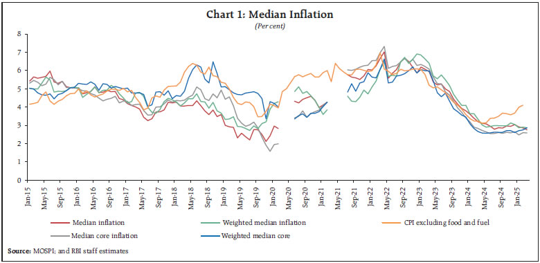

The MCT measure of inflation can be helpful in tracking headline for countries where food and fuel inflation are volatile and has significant weight in the headline inflation. The concept of MCT measure, based on the methodology proposed by Stock and Watson (2016), is popularised by the Federal Reserve Bank of New York (FRBNY) after Almuzara and Sbordone (2022) published an article in Liberty Street Economics to explain the sources of inflation surge in the post-pandemic period. The FRBNY publishes the MCT inflation for the US on Monday following the release of the PCE data. The MCT inflation measure accounts for time-varying weights influenced by the volatility, persistence, and co-movement of different sectoral inflation. Inflation of each sector is decomposed into four components: a common trend, a sector-specific trend, a common transitory shock, and a sector-specific transitory shock. CPI inflation trend is estimated by adding the common trend with the sector-specific trends weighted by the CPI Core weights. Trend decomposition can further help identify the source of inflation persistence (Almuzara and Sbordone (2022)). The persistence and spillover from the volatile components of the CPI contributes to MCT inflation through the common trend.

There has been series of studies in the Bulletin of Reserve Bank of India around alternate core measures. Patra et al., (2024a) investigates core-like properties of food inflation, viz. volatility, persistence, spillovers and cyclical sensitivity. George et al., (2024) investigates several core measures based on exclusion, trimmed means, reweighted CPI, and trend CPI (HP, CF, PCA etc). However, the inflation measure introduced in this paper captures the time varying persistence and second round effects² of the inflation components in the multivariate core trend (MCT). The inclusion of the contribution from volatile component, food and fuel, through common trend, is further justified by Patra et al., (2024b) which provides empirical evidence to suggest the spillover from food inflation to non-food components.

IV. Model Description

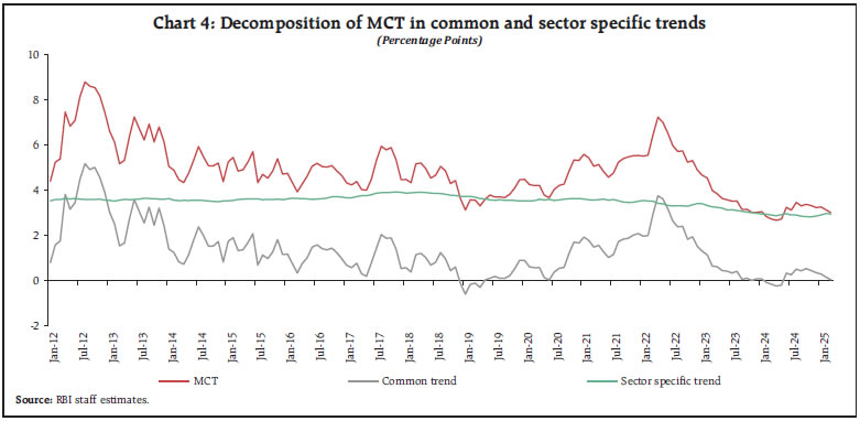
Where the disturbances (η_τ,c,t, η_ϵ,c,t, η_τ,i,t, η_ϵ,i,t, ζ_i,τ,t, ζ_i,ϵ,t, ν_Δτ,c,t, ν_ϵ,c,t, ν_Δτ,i,t, ν_ϵ,i,t) are independent and identically distributed standard normal. The multivariate model allows the outliers in inflation, which occur each period with probability p_c and p_i, respectively in common shocks and sector specific shocks, through independent and identically distributed normal random variables s_c and s_i (Stock and Watson, 2016).

The aggregate trend inflation (τ_t) is given by weighted sum of the sectoral trends where w_i is the weight or contribution of i^th sector in the combined consumer price index.

V. Empirical Results

We estimate MCT inflation for India using item-level CPI data from January 2012 to March 2025. The 9-digit-level CPI items are grouped into 23 subcategories: 12 under Food and Beverages, 6 under Miscellaneous, 2 under Clothing and Footwear, and one each under Pan, Tobacco and Intoxicants, Housing, and Fuel and Light⁴. Using the methodology outlined in the previous section and sub-group level CPI weights, we compute MCT inflation for India.

Before turning to the multivariate trend estimates, we first estimate univariate measures of trend inflation using the Unobserved Components model with Stochastic Volatility and Outlier Adjustments (UCSVO), applied separately to headline and core CPI. The UCSVO specification mirrors the MUCSVO model but excludes the common shock or common trend structure⁵. The univariate trend estimates suggest that inflation was generally on a declining trajectory until the starting of the COVID-19 pandemic (Chart 2). Supply disruptions during the pandemic and the Ukraine war led to a temporary rise in trend inflation until end-2022. Subsequently, trend inflation declined, reaching 4.3 per cent by March 2025.

The UCSVO results also indicate that the volatility of trend in headline CPI is higher than that of core inflation, reflecting the persistence of food and energy shocks⁶. This highlights the potential bias in conventional core inflation measures that exclude food and fuel components without accounting for their persistent effects (Stock and Watson, 2016; Manopimoke and Limjaroenrat, 2017). However, the temporary rise in stochastic volatility in core trend inflation reflects pandemic and war related supply disruptions that affected core services and goods, not just food and fuel. Elevated logistics costs, medical expenses, and administered price adjustments widened inflation persistence across core items, blurring the historical separation between volatile and “sticky” CPI groups.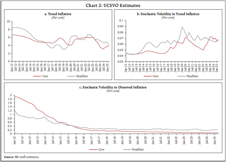

For both core and headline CPI, the stochastic volatility of observed inflation remains higher than that of the trend inflation, though both have declined steadily over time. Interestingly, volatility in core inflation was initially higher than headline inflation but reversed after September 2015.

To estimate MCT inflation, we use only the core CPI components, with their weights normalised to one. While these core weights are fixed, sectoral contributions vary over time due to time-varying coefficients on the common trend (α_i,τ,t). The estimated MCT inflation is considerably smoother and less volatile than both headline and core CPI (Chart 3). Between January 2012 and March 2025, headline inflation had a volatility of 2.16, core inflation 1.59, and MCT inflation of just 1.25. Although core CPI and MCT inflation tend to move together, core CPI appears to lag MCT. Both measures have remained below 4 per cent in recent months. MCT inflation rose from April 2019 to April 2022, then declined, suggesting a fall in inflation persistence.

To understand this recent decline in trend inflation, we decompose MCT inflation into common and sector-specific components. Each subgroup contributes to MCT through two channels: a common trend and a subgroup-specific trend. The common trend captures persistent shocks, including those from food and fuel, while the subgroup-specific trends reflect stickiness of core CPI components. This structure allows MCT to capture second-round effects more effectively than traditional core inflation measures. The contribution of common trend in MCT depends on the time varying weight attached to the trend component. Thus, contribution of any specific sector to MCT inflation comprise of both common trend component and its own trend component (Chart 4). While subgroup-specific contributions are relatively stable, changes in the common trend – comprising both volatile components (food and fuel) and more stable components (core) – largely determine the dynamics of MCT.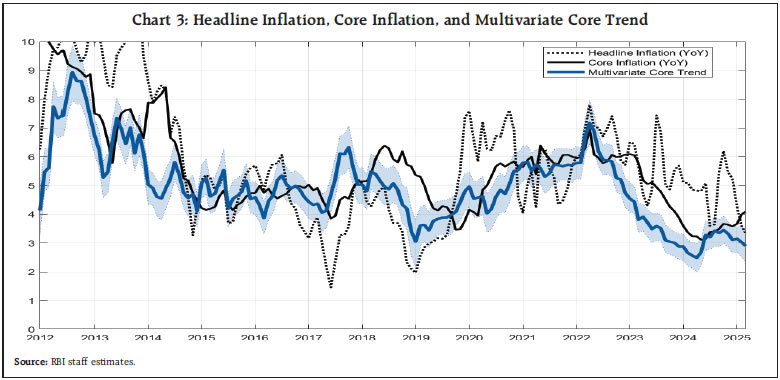

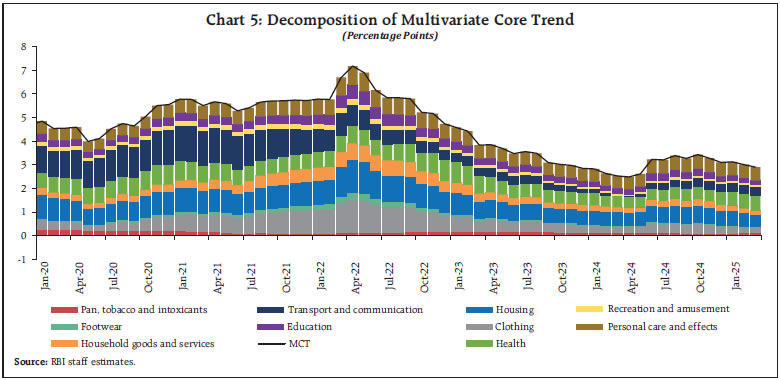A further decomposition reveals that contributions from transport and communication, clothing, and household goods and services have declined over time, while the role of personal care and effects has increased (Chart 5). This changing composition offers insight into the evolving sources of inflation persistence.

We also explore a less granular decomposition by aggregating subgroups into broader categories: clothing and footwear together with pan, tobacco and intoxicants; housing; and miscellaneous. Contributions from each major group are derived from their constituent subgroups. MCT inflation estimated from group-level components differs from that aggregated from subgroup-level estimates, due to differences in both common and sector specific trend dynamics. The results show a clear declining contribution of clothing and footwear and a recent increase in contribution of miscellaneous categories to overall MCT inflation (Chart 6).

Additionally, we classify inflation into goods and services: core goods, core services, non-core goods, and non-core services. Table 2 presents the number of items and their respective weights in each category.

The decomposition of MCT inflation by goods and services reveals no significant shift in contribution patterns overall (Chart 7). However, while goods historically contributed more to MCT, the share of services has risen in recent months.

This version of MCT inflation, constructed using goods and services decomposition, is also smoother than core and headline CPI inflation. Between January 2015 and March 2025, headline and core CPI inflation had volatilities of 1.39 and 0.91, respectively, compared to just 0.69 for MCT inflation. Table 3 summarises the descriptive statistics of all inflation measures, with MCT2 covering the period from January 2015 to March 2025.

VI. Predictive Power

We assess the predictive power of MCT inflation in forecasting both core and headline inflation. Forecast performance is evaluated using out-of-sample root mean square error (RMSE) for different time horizons (1, 3, 6, and 12 months ahead). Lower RMSE values imply better predictive accuracy. A baseline model using the most recent observed value of headline inflation (i.e., a random walk) is used as a benchmark, with its RMSE normalized to 1. Relative RMSEs for other models are then calculated.

Forecasts are evaluated over the test set from April 2024 to March 2025 using rolling RMSEs. Results show that MCT significantly improves forecast performance, particularly for core inflation, and consistently outperforms the benchmark across all horizons. For headline inflation, MCT improves long-horizon forecasts, but gains are limited at shorter horizons –likely due to its focus on persistent trends rather than short-term volatility in non-core items. Notably, forecasts based on MCT2 (estimated from goods and services decomposition) outperform the broader MCT model (Table 4).

VII. Conclusion

This paper develops a Multivariate Core Trend (MCT) inflation measure for India using a Bayesian multivariate unobserved‑components model with stochastic volatility, calibrated on disaggregated CPI components. The MCT framework provides a structural advantage over exclusion‑based core inflation metrics by allowing time‑varying sectoral sensitivities, explicitly modelling both common and idiosyncratic trends, and capturing second‑round effects from food and fuel through the common trend channel.

Empirically, MCT inflation is smoother and less volatile than both headline and conventional core inflation. It leads core inflation during turning points, suggesting its usefulness as an early signal of evolving inflation persistence. The decomposition shows that the common trend – combining persistent pressures from both core and volatile components – explains much of the recent inflation cycle, with sector‑specific persistence relatively stable. Notably, services inflation has gradually become a more prominent contributor to the MCT in the post‑pandemic period, consistent with evolving consumption patterns and supply‑chain normalisation.

Forecast evaluation confirms the usefulness of MCT: although short‑horizon gains are modest, MCT demonstrates superior predictive accuracy for core inflation at medium‑ and long‑term horizons, outperforming random‑walk and conventional core benchmarks. These results reinforce the importance of using flexible, disaggregated trend‑extraction frameworks when commodity‑price shocks and supply‑chain rigidities drive headline inflation dynamics.

However, MCT measure is not simple to interpret, and is difficult to communicate. Further, the choice of disaggregation can have impact on the MCT measure. The MCT decomposition can be used for tracking early signal of persistence and second round effects of inflation components.

Overall, the findings suggest that MCT inflation is a robust operational measure of underlying inflation pressures and can complement existing core measures in India’s monetary policy framework. Future work can explore high‑frequency extensions, real‑time filtering properties, and state‑dependent dynamics – particularly for differentiating supply‑driven and demand‑driven inflation persistence in India’s evolving macro‑financial environment.

References

Almuzara, M. and Sbordone, A. (2022) Inflation Persistence: How Much Is There and Where Is It Coming From?, Federal Reserve Bank of New York, Liberty Street Economics, April 20, 2022, Retrieved from https://libertystreeteconomics.newyorkfed.org/2022/04/inflation-persistence-how-much-is-there-and-where-is-it-coming-from/.

Apel, M., and Jansson, P. (1999), A Parametric Approach for Estimating Core Inflation and Interpreting the Inflation Process, Stockholm, Sweden, Sveriges Riksbank Working Paper Series, 80.

Behera, H. K., & Patra, M. D. (2022), Measuring Trend Inflation in India. Journal of Asian Economics, 80, 101474.

Behera, H. K. & Ranjan, A. (2024), Food and Fuel Prices: Second Round Effects on Headline Inflation in India, RBI Bulletin, April, 2024.

Blinder, A.S. (1982). The Anatomy of Double-Digit Inflation in the 1970s. In R.E. Hall (ed.), Inflation: Causes and Effects, 261-282, University of Chicago Press.

Chhibber, A. (2020), With Food and Fuel Consumer Price Index Surges, it’s Time to Rethink the Inflation Target Regime, Economic Times (24 January, 2020).

Eckstein, O. (1981). Core Inflation, Engelwood Cliffs, N.J, Prentice-Hall 1981.

Eichengreen, B., & Gupta, P. (2024) Inflation Targeting in India: A Further Assessment, NCAER Working Paper #174.

George, A.T., Bhatia, S., John, J. & Das, P. (2024), Headline and Core Inflation Dynamics: Have the Recent Shocks Changed the Core Inflation Properties for India?, RBI Bulletin, February, 2024.

Manopimoke, P., & Limjaroenrat, V. (2017). Trend inflation estimates for Thailand from disaggregated data. Economic Modelling, 65, 75-94.

Ministry of Finance (2024), Economic Survey 2023-24, New Delhi: Ministry of Finance, Department of Economic Affairs.

Patra, M.D., John, J. & George, A.T. (2024a), Are Food Prices the ‘True’ Core of India’s Inflation?, RBI Bulletin, January, 2024.

Patra, M.D., John, J. & George, A.T. (2024b), Are Food Prices Spilling Over?, RBI Bulletin, August, 2024.

Stock, J.H., Watson, M.W., (2007). Why has US inflation become harder to forecast? Journal of Money, Credit & Banking 39 (s1), 3-33.

Stock, J.H., Watson, M.W., (2016). Core inflation and trend inflation. The Review of Economics and Statistics 98 (4), 770-784.

Appendix

Data

The Ministry of Statistics and Program Implementation (MOSPI) release inflation data on 12th day⁷ of every month. The press release reports headline, and food inflation for India. It also releases disaggregated item level inflation data on its website. Each item has 9-digit code, and the coding structure has been devised such that each item is identified uniquely in various sub-grouping. 1st digit represents ‘Group’, 2nd digit represents ‘Category’ within the group, 3rd and 4th digits represent ‘Sub-group’ for every group, 5th digit represents ‘Section’, 6th digit represents ‘Goods/Services’, 7th and 8th digits gives item serial number within Section and 9th digit represents identification of items: Weighted Item or Priced Item. A sample of the items along with the code is provided in Table A1⁸.

1st digit which represents group are summarized in Table A2. Core inflation is obtained by removing Group 1 (Food and Beverages), and Group 5 (Fuel and Light).

2nd digit represents category within the group. For example, within Group 1, there are two categories: Food and Beverages. The code 1.1 represents Food whereas 1.2 represents Beverages. 3rd and 4th digit represents subgrouping within a group. For example, Food and Beverages are further subgrouped in Cereal and Products, Meat and Fish, Egg, Milk and Products, Oils and Fats, Fruits, Vegetables, Pulses and Products, Sugar and Confectionery, Spices, Non-alcoholic Beverages, and Prepared meals, snacks, sweets etc. Similarly other groups can be classified into different subgroups⁹. 5th digit is the section within subgroup. For example, Cereal and Products are further subclassified into different sections: Major cereals and products, Coarse cereals and products, and Grinding charges. 6th digit is 1 or 2 based on the item type. 1 represents Goods, whereas 2 is for Services. 7th and 8th digit is for the item serial number within section. 9th digit is identification type. 9th digit can be ‘X’, ‘P’ or ‘0’. ‘X’ is for an item if it has more than one priced item, ‘P’ is for PDS items, and ‘0’ for all remaining items. MOSPI (2015) provides full details of the classification. We use this 9-digit code to compute different Multivariate Core Trend Inflation.

The disaggregated subgroups along with their weights are provided in the Table A3.

^{^} The authors are from the Department of Economic and Policy Research, Reserve Bank of India. The views expressed in this article are those of the authors and do not represent the views of the Reserve Bank of India.

¹ Core inflation in India is commonly defined as CPI excluding food & beverages and fuel & light. Alternative operational definitions – such as excluding only food or excluding volatile subgroups – exist in literature but are not used in this baseline specification.

² Behera, H. K. & Ranjan, A. (2024), “Food and Fuel Prices: Second Round Effects on Headline Inflation in India” RBI Bulletin, April

³ For detailed estimation approach including choice of number of iteration and burnouts, please refer to online appendix of Stock and Watson (2016). https://www.princeton.edu/~mwatson/papers/core_and_trend_inflation_online_appendix_20151103.pdf

⁴ Details of data and sectoral weights are provided in the Appendix.

⁵ See more Stock and Watson (2016) for more details on UCSVO.

⁶ Model-detected outliers align with major macroeconomic disruptions: (i) nationwide lockdown and mobility restrictions (Q1-Q2 2020), (ii) supply chain normalisation with inventory restocking (late-2020), and (iii) global energy and commodity price surge after the Russia-Ukraine war (2022). These outliers reflect non-systematic, high-amplitude price movements that do not represent persistent inflation dynamics.

⁷ In case of weekend, it releases either on 11th or 13th day of the month.

⁸ For complete table along with their weights, please refer to https://cpi.mospi.gov.in/Weight_AI_Item_Combined_2012.aspx

⁹ For full classification, please refer MOSPI (2015).