Press Release RBI Working Paper Series No. 03 Monetary Policy Transparency and Anchoring of Inflation Expectations in India G. P. Samanta and Shweta Kumari@ Abstract * This study provides a measure of the degree of monetary policy transparency in India using text-mining techniques and, examines the impact of transparency on anchoring of inflation expectations. Inflation expectations are sourced from two RBI surveys - Survey of Professional Forecasters and Survey of Inflation Expectations of Households. The transparency level appears to have increased substantially since India adopted a flexible inflation targeting framework. Further, we assess if improved transparency has any impact on the degree of anchoring of inflation expectations. Though the expectation anchoring has been defined in several ways in the literature, we describe the concept in terms of sensitivity of expectations to available information. In this process, depending on the underlying information set, we consider the aspect of expectation anchoring in three categories, viz., weak-form, semi-strong-form and strong-form, and focused on the weak-form for empirical analysis. We find that the enhanced transparency is associated with improved weak-form anchoring of inflation expectations by professional forecasters well within the inflation tolerance band. Households' expectations are also found to be anchored in weak-form but at a level higher than the inflation target. JEL Classification: E500, E520, E580 Keywords: Policy transparency, survey-based inflation expectations, expectations anchoring, dummy variable regression, rolling regression Introduction Central bank transparency is key to building credibility and anchoring inflation expectations in the era of modern monetary policy-making. Keeping the public and markets informed and updated about the actions being taken to achieve the stated goals is one of the strategies practised widely by central banks across the globe, but the extent of transparency may vary from one central bank to another. Greater transparency may improve the effectiveness of monetary policy in several possible ways. First, it makes central banks more accountable, thereby creating a potential scope for enhanced credibility. Second, transparent and credible policy actions can influence market expectations to stabilise/ align their movements with stated policy targets. Further, in situations when a central bank needs to take unconventional policy actions, proper explanation of the rationale for such actions combined with credibility earned beforehand can help the market and other stakeholders to understand the situation and avoid any hasty reaction. So, transparency may enhance flexibility in policy-making. In India too, central bank communication, especially those related to monetary policy receives extensive coverage, in print media, social networks and TV channels. The policy decisions taken by the Reserve Bank of India (RBI) and communications on the outlook for the near future are widely sought after, along with the rationale behind such decisions and deliberations. RBI, for over more than a decade, has been putting efforts to improve the transparency, even before adopting flexible inflation targeting (FIT), by disclosure of relevant information, such as detailed policy review, publication of monetary policy surveys' results, forecasts of growth and inflation with the balance of risk and risk factors. The ';Expert Committee to Revise and Strengthen the Monetary Policy Framework'; (Chairman: Dr Urjit R Patel) in its 2014 report ('EC2014' hereafter) also emphasised on the importance of communication and transparency for monetary policy framework and recommended publishing frequent macro-economic assessment and clarify the policy stance, to enhance policy effectiveness and contain destabilising expectations. Central banks' communication and policy transparency have been key instruments for strengthening accountability and enhanced credibility, and for anchoring inflation expectations by promoting understanding of monetary policy (Blinder et al., 2008; Hubert, 2015; Rajan, 2013). In this context, it may be imperative to measure the degree of RBI's monetary policy transparency, its efficacy and role with regards to broader policy objectives. Against this background, this study attempts to (a) quantify the monetary policy transparency in India; (b) understand how the transparency level evolve; and (c) examine if transparency facilitated the anchoring of inflation expectations. We follow the methodology developed by Eijffinger and Geraats (2006), hereafter referred to as 'EG Methodology', based on the theoretical background, and construct an index which measures the monetary policy transparency in India. However, there are two noticeable differences: (i) instead of annual estimates of transparency index, a more frequent measure of transparency has been computed for every policy review window; and (ii) usage of big data techniques (especially text mining capabilities) to help in the reading of policy statements and other relevant documents (instead of complete manual reading). As mentioned by Warsh (2014) in a review of Bank of England's transparency practices, ';the most transparent central bank is not necessarily owed a gold star. That distinction is owed to the central bank, which makes the best decisions, effectively communicates those decisions, is held to account for its actions, and provides the fairest and most accurate historical record';. Taking a cue from this, we do not deliberate upon whether greater transparency is better or worse in the Indian context or determine an optimal level of transparency. Instead, we estimate the transparency of monetary policy as it has evolved over time and assess its likely impact on the anchoring of inflation expectations. We consider inflation forecasts as obtained in the Survey of Professional Forecasters (SPF) and inflation expectations as obtained in the Inflation Expectations Survey of Households (IESH) conducted by RBI in this study. The methodological framework adopted for analysing dynamics of inflation expectation and realised inflation in the presence of higher central bank transparency is due to Cruijsen and Demertzis (2005). The rest of the paper is structured as follows. Section II provides a review of relevant literature, covering monetary policy transparency as well as anchoring of inflation expectations. The methodology of construction of monetary policy transparency index along with measured transparency, and the significant factors contributing towards changes in the level of transparency are discussed in Section III. The data, methodology for analysing the anchoring of inflation expectations in the presence of transparency, and empirical results are presented in Section IV. Section V concludes. II. Literature Review: Policy Transparency and Inflation Expectations Anchoring For central banks across the globe, inflation is a matter of concern, more so for inflation targeting countries. The realised inflation is closely linked to inflation expectations as suggested by numerous studies in the literature. Anchoring inflation expectations is, therefore, considered as one of the significant steps to keep inflation within the target zone, and accordingly it has gained importance in the context of monetary policy, particularly for inflation-targeting central banks. Further, a broad consensus has also emerged in the central banking literature on the desirability of transparency in central bank policy and communication. II.1 Measuring Policy Transparency Measuring policy transparency is a challenging task primarily because it is a qualitative concept and burdened with subjectivity. In literature, there are a few techniques for measurement of transparency. Bini-Smaghi and Gros (2001) made an early attempt to construct an indicator of central bank transparency and accountability. They consider transparency under four significant aspects viz., goal and its quantification, strategy to achieve it, the publication of data and forecast, and communication strategy. One of the widely used approaches is due to Eijffinger and Geraats (2006) (EG hereafter), who suggest an analytical framework with theoretical background and estimate policy transparency index for nine central banks at annual frequency for the period 1998-2002. They divide central bank transparency under major five dimensions or aspects viz., political, economic, procedural, policy and operational, with a rationale that different aspects play different roles in monetary policy decision. They create a transparency index by quantifying, i.e., assigning scores on a set of three questions under each dimension. Dincer and Eichengreen (2014) replicate the EG methodology and construct the transparency index for more than 100 central banks for a longer time horizon, at annual frequency from 1998 to 2010. A review of Bank of England transparency practices (Warsh, 2014) also employs the transparency indices provided by Dincer and Eichengreen (updated up to 2014). They provide details on various aspects of transparency. As regards India, the quantitative measure of monetary policy transparency is scarce in the existing literature. Though Dincer and Eichengreen (2014) included India among the 100 central banks for their study (1998 to 2010), no explanation is provided for the scores assigned. Oikonomou and Spyromitros (2017) update the transparency index for 34 countries over the period from 2011 to 2016, including India, but again the rationale for the score allotted by them for India are not available. II.2 Anchoring of Inflation Expectations The degree of inflation expectations anchoring is vital because it affects inflation and other macroeconomic factors in general. The degree to which the expectations remain anchored may also reflect on commitment and credibility of a central bank. The topic of inflation expectations and its anchoring; therefore, has been a critical theme of many studies across the world, we only list a few studies. II.2.1 Defining Expectation Anchoring: Conceptual Issues Inflation expectation anchoring is a complex topic, and defining it is not straightforward. There are two broad approaches to defining and assessing the degree of inflation expectation anchoring. First, examining if inflation expectations or forecasts are indifferent to changing economic scenarios as reflected in the behaviour of one or more macro-economic variables. It merely says that the extent to which inflation expectations change given a change in economic conditions determines the degree of non-anchoring of expectations1. In other words, if expectations are not anchored, any (surprise) change in relevant variables or information at a given time will affect inflation expectations in the subsequent period to a great extent. Thus, inflation expectations may be said to be well anchored when they are relatively less sensitive to (unexpected) change in a set of variables representing economic conditions. In the simplest form, survey-based inflation expectations are regressed on any change in inflation. If anchored, inflation expectation will not be affected by realised inflation. The second approach defines inflation expectations in terms of technical aspects of convergence and consistency of expectations across respondents or time points/horizons. For example, five alternative definitions of anchored expectations, viz., ideally anchored, strongly anchored, weakly anchored, consistently anchored, and increasingly anchored, defined by Kumar et al. (2015), fall under this category. These definitions are grounded with strong analytical concepts and examine whether or how fast the expectations converge to either the central bank's target or other constant value that would emerge as the implicit consensus among the target group of respondents. II.2.2 Time Horizon of Inflation Expectations Inflation expectation anchoring is mostly studied regarding medium to long-term expectation sensitivity. However, as pointed out by Lyziak and Paloviita (2016), policy decisions and communication by a credible central bank can also influence short-and-medium-term inflation forecasts, which are important in the context of wage and price setting. Further, owing to data limitation due to non-availability of long-term inflation expectations, some studies have assessed the degree of expectation anchoring based on short-run inflation forecasts. For example, Lyziak and Paloviita (2016) carried out empirical analyses based on only one-year ahead inflation expectation from consumers' survey though used short-to-long run forecasts for the survey of professional forecasters. II.2.3 Empirical Literature: Inflation Expectations Anchoring Empirical studies available in the literature adopted various approaches to assess the degree of inflation expectation anchoring. In an early attempt, Levin et al. (2004), in a study of 12 central banks, examine the extent to which the inflation targeting regime significantly influences the expectation formation and inflation dynamics. They observe that the inflation targeting regime helps agents to form expectations, as the linkage between expectation and actual inflation weakens resulting in a higher degree of anchoring. Cruijsen and Demertzis (2005) analyse the dynamics of inflation expectation and realised inflation in the presence of higher central bank transparency for eight industrialised countries and the Euro Zone. They conclude that central banks with higher transparency are better able to anchor inflation expectations. Demertzis and Hallett (2007) present the evidence for nine OECD countries that transparency helped reduce the inflation variability, among other significant results. Later, Dincer and Eichengreen (2014) also obtained similar results for 100 central banks. Geraats (2009), while elaborating a theoretical framework of central bank transparency, analyses transparency trends across various monetary policy frameworks practised in different countries. It finds, inter alia, that lower average inflation follows a higher level of transparency. Patra and Ray (2010) explore the causal factors of inflation expectations in India and find that past inflation, as well as the real interest rate, has a significant impact on inflation perceptions. They generate inflation expectations using a model-based approach and also from Consensus Economics (through a survey covering financial entities), in the absence of long time-series data of inflation expectations from surveys at that point of time. Sousa and Yetman (2016) provide evidence that inflation expectations in emerging market economies (including India) have become more anchored over time, by estimating a long-term anchor for each country and estimating the sensitivity of inflation expectation to this anchor. A slightly different approach is adopted in Lyziak and Paloviita (2016), where they define anchoring as the ability of the European Central Bank (ECB) to manage inflation expectations, assessed in terms of communication tools such as the set target and inflation projections, in addition to sensitivity to actual inflation. Using aggregated quarterly survey data (both consumer and professional forecasters), they assess the degree of anchoring in the euro area and find evidence of de-anchoring in a recent period. Carvalho et al. (2017) examine anchoring defined in terms of linkage of long-term inflation expectations with short-term expectations. They find that the extent to which anchoring takes place may vary from time to time depending on the conduct of monetary policy and other economic developments, as observed for the US and some other countries. A recent study by Choi et al. (2018) assess inflation anchoring in terms of sensitivity of medium-term expectations to inflation shocks and go one step further to evaluate the effect of inflation anchoring on growth. They use survey-based measures of inflation expectations from Consensus Economics for 36 economies, including India. III. Monetary Policy Transparency Index for India Transparency is a qualitative concept and comes with inherent subjectivity, and therefore its quantification is a challenging task. Although RBI had been continuously working on to enhance the transparency by way of more information disclosure, the majority of the decisions to improve communication and transparency were recommended by the EC2014. Like many peer central banks, RBI specifies its goals and approach towards achieving the same. It provides the rationale for its policy decision by providing an assessment of the domestic and global macroeconomic situation. Besides, it also guides the near future outlook for the economy covering five-quarter forecasts for inflation and output, together with upside and downside risks associated with such forecasts. Even the dates of the Monetary Policy Committee (MPC) meetings and the release of policy decision are announced beforehand. By providing guidance to the general public, media, financial markets and other stakeholders and keeping surprise elements at bay, considerable importance is given to prudent communication and transparency. We adopt the analytical framework suggested by Eijffinger and Geraats (2006) and applied subsequently by Dincer and Eichengreen (2014) and Warsh (2014), for the construction of a monetary policy transparency index for India. The choice of using this framework is primarily driven by the theoretical background, descriptive questions and clarity of scoring mechanism for various questions. III.1 The EG Methodology The approach due to Eijffinger and Geraats (2006) is quite comprehensive as it covers various dimensions of transparency and provides a logical framework, which starts with a target to be achieved by monetary policy and ends with whether there is an assessment of the policy decisions about the accomplishment of the set target, as explained in Chart 1. Overall, there are five broad categories, consisting of three questions each, as summarised in Chart 2. The broad categories and the various questions are detailed in Annex I. Each question has multiple choice answers with a score of 0, 0.5 or 1, so the score of each category can be in the range of 0 to 3. Scores of five categories are then summed up to compute the overall transparency Index, which can range from 0 to 15. III.2 Measuring RBI's Monetary Policy Transparency Eijffinger and Geraats (2006), scanned the information published by central banks and government authorities. The computed scores were then shared with various central banks for review, based on which they reassessed the scores and made a few modifications. Dincer and Eichengreen (2014), collect information from central banks' websites, annual reports, and other published documents. For the present study, we use the information released by the RBI as contained in the Monetary Policy Statements, Monetary Policy Reports (MPR), Minutes of Monetary Policy Committee (MPC) meetings, erstwhile Macroeconomic and Monetary Developments (MMD) Reports and Minutes of Meeting of Technical Advisory Committee on Monetary Policy (TACMP), together with a few other reference documents form the data corpus, which was analysed for construction of Transparency Index (TRP Index). We consider the period of about a decade: from October 2009 to February 20192 for our study, to understand the dynamics of monetary policy transparency in various aspects. The basic premise of transparency is the release of information to the public, and therefore, only publicly available documents have been considered in the study, approximately 100 documents, all sourced from RBI website. During the period under study, RBI moved from quarterly policy reviews to the addition of mid-quarter reviews (in September 2010), to the current practice of bi-monthly reviews (since April 2014). In view of this change and to maintain consistency, we present the TRP index on monthly frequency where the value of TRP index for intervening months (between consecutive quarterly/bi-monthly policy reviews) is kept same as the previous value. III.2.1 Leveraging on Big Data techniques – Utilising Text Mining Techniques Reading these documents, which are available primarily in text form, and quantifying the answers to various questions for construction of transparency index is a tedious task and may consume considerable time. However, some major developments and events on the relevant areas are usually common knowledge, though there might be a possibility that details of some events are not readily available. So, to overcome possible overlooking of such events, we broadly followed a two-step process. In the first step, we let the big data and text mining techniques to read various documents automatically. In the second step, we manually recheck some of the events triggered/identified in the first step. Since each question is unique (please refer to Annex I for details), appropriate heuristic methods were adopted to find the answer and score the question. An indigenous program code was developed in the R programming language to automatically score each question using regular expressions. The scores of various questions in the five categories were added to get the overall TRP Index. The program code was then reiterated many times to process all documents from October 2009 to February 2019. It may be comparatively more straightforward for subject matter (monetary policy) experts to be able to provide answers to the various questions without manually scanning many reference documents; however, reading the numerous documents to find scores and estimation of transparency index may be a tedious task otherwise. Text Mining technique offers many advantages, viz. automatic scanning of reference documents, question by question scoring, ability to scan documents across periods, thus, saving time and minimising subjective bias. The technique may be regarded as useful if the derived estimate of transparency index can identify the changes taking place in monetary policy regime from time to time; otherwise, its scope would be limiting in nature. In the study, the change points identified by the estimated transparency index pertain to significant changes taken place in monetary policy area in India (as would be seen in a later section) implying the usefulness of text mining capabilities. Furthermore, we estimate a few variants of transparency index to address the issue of subjectivity in some aspects, as described in the next section. III.2.2 Monetary Policy Transparency Index As the notion of transparency is subjective, and its accurate measurement is challenging, we estimate a few variants of transparency index. This is done by altering scores of some questions, which are comparatively more subjective and re-estimate the index. Four variants of TRP index (denoted by TRP Index V1 to TRP Index V4) are plotted in Chart 33. As observed, their patterns broadly remain the same. Further, the time point of changes, is similar in different variants, except in the second variant where the second change did not occur. Major differences among different variants in terms of category wise scores are presented in Annex I. We find evidence of six changes in the transparency for the first variant of TRP Index, as described in Table 1, however since the latest change occurred in October 2018 resulting in the limited number of observations after that in our study period, we combine it with previous regime change. Accordingly, we exclude the sixth change point in transparency listed in Table 1 from empirical analysis. | Table 1: Changes in TRP Indexes | | Sr. No. | Starting period for possible change/ jump in TRP Indexes | Corresponding Quarter | | 1 | January 2011 | January-March 2011 | | 2 | October 2011 | October-December 2011 | | 3 | April 2014 | April-June 2014 | | 4 | April 2015 | April-June 2015 | | 5 | October 2016 | October-December 2016 | | 6 | October 2018 | October-December 2018 | | Note: For more information on the change in transparency, please refer to Annex I. | It is observed that transparency received a significant boost in April 2014, when some of the recommendations of EC2014 were implemented including the adoption of Consumer Price Index (CPI) based headline inflation as inflation measure and explicit recognition of disinflationary glide path. The TRP indexes remained low within 6-8.5 till the quarter of Oct-Dec. 2013 before witnessing a big jump in Apr-Jun 2014 quarter; passed through a transition phase of a couple of two other jumps to reach a new high level of 12-13 in the quarter Oct-Dec 2016 and remained stable around that level for the major part of the period thereafter. Interestingly, as we shall see later, the transition phase, by and large, coincides with the period of glide path in inflation target followed by the RBI. Noting that different variants of computed transparency indexes are broadly similar, we describe Variant 1, i.e. TRP Index V1, in detail in subsequent paragraphs. Chart 4 presents the first variant of transparency index together with its' disaggregated category wise scores for the period under study. It is observed that the transparency has increased considerably during the period from 6.5 to 13-14. Notably, transparency has increased significantly in almost all aspects. Now we discuss each aspect of transparency and the crucial factors which contributed to changes in scores over the period under study. Mandate/ Political transparency – Before April 2014, multiple indicator approach was followed where in addition to inflation, money, credit, output, trade, capital flows, fiscal situation, exchange rate, etc. were considered while taking monetary policy decisions. Since there was no defined prioritisation among these indicators, and no numeric values were set as a target, the transparency score was zero for such periods. Following the recommendations of EC2014, RBI had self-imposed targets as it adopted disinflationary glide path with targets of 8 per cent by the end-2014, 6 per cent by end-2015 and 5 per cent by end-2016 (see Patra, 2017). This was also announced in the monetary policy statement of April 2014, ';The Reserve Bank's policy stance will be firmly focused on keeping the economy on a disinflationary glide path that is intended to hit 8 per cent CPI inflation by January 2015 and 6 per cent by January 2016';. Setting up quantitative targets helped in improving the political transparency score from zero to two (starting from April 2014). Under flexible inflation targeting (FIT) framework, starting from the financial year 2016-17, the inflation target in India is set at 4 per cent with the lower threshold of 2 per cent and the upper threshold of 6 per cent, for the period up to March 2021. The move towards the FIT framework was formalised by ';Monetary Policy Framework Agreement (MPFA) by Government of India and RBI'; in February 20154, which further takes up the score to three. Accordingly, full three marks are allotted in political transparency since April 2015 (this was the first monetary policy announcement after MPFA came into place in February 2015). Economic transparency – EG Methodology suggests checking whether time-series data of key macroeconomic variables used as input for monetary policy is published, by the central bank or outside entity. They indicate five key variables viz., money supply, inflation, GDP, unemployment rate and capacity utilisation. However, it is natural that depending on the country-specific characteristics or the period under consideration, some of these variables may be replaced by the similar but more relevant/ significant variable. For example, in India, although data on money supply are available, liquidity is considered more relevant as an input to the monetary policy decision, since monetary policy operating framework is designed in terms of liquidity. An official measure of the unemployment rate is not available in India. However, there exist some proxies in terms of wage growth data, unemployment rate published by Centre for Monitoring Indian Economy (CMIE) and employment-related qualitative information for the manufacturing sector from Industrial Outlook Survey (IOS)5. Time series data on Capacity utilisation is available from Order Books, Inventories and Capacity Utilisation Survey (OBICUS) and also from IOS. Time series data on all variables under consideration are publicly available. While the data on GDP, Inflation, wage are sourced from the Central Statistics Office (CSO), Ministry of Statistics and Programme Implementation (MOSPI), Government of India (GOI), the data on OBICUS, IOS and liquidity (weighted average call rate, repo rate etc.) are released by RBI on a regular basis. All these data are available throughout the study period, except OBICUS which started getting published since October 2011, resulting in a full score for the first question of economic transparency, and one-half for earlier periods (prior to October 2011). Next question relates to disclosure of the policy model adopted internally. Although reference of a Quarterly Projection Model / Structural and other models occurs in the reference documents from time to time, it was only in MPR of October 2018 that an explicit reference was made towards ';Quarterly Projection Model for India: Key Elements and Properties'; (Benes et al. 2016) that the Reserve Bank uses for policy analysis and internal forecasts. Accordingly, the score comes out to be zero for the significant part of the period under consideration. The third question relates to whether the central bank releases internal macroeconomic forecasts. In this area, full marks are allotted for the entire study period, as RBI promptly releases numeric internal forecasts for inflation as well as output with each policy review statement, and also provides fan charts of internal projections for the medium term. In addition to the forecasts, underlying assumptions together with the balance of risk (both upward and downward) are also mentioned. Procedural transparency – This aspect begins with whether there is an explicit monetary policy rule or strategy describing the monetary policy framework6. Operating framework of monetary policy is in place during the study period. It is, therefore, appropriate to assign full score on this aspect7. The decision on key policy instrument (repo rate) is currently taken by the MPC and the minutes are published on the fourteenth day after every MPC meeting. These minutes are quite comprehensive and unique in the sense that it also consists of statements providing rationale for their individual votes, by all members, in the resolution adopted (i.e. the decision to increase, decrease or hold the policy rate). The information on the inputs considered by the MPC for such decision, e.g. internal macroeconomic projections along with risks, combined with indications coming out of various monetary policy surveys is also provided in the minutes and forward-looking arguments. However, before MPC came into existence, there was a Technical Advisory Committee on Monetary Policy (TACMP), whose role was advisory in nature without any voting rights. Although the TACMP was constituted in 2005, it was only in January 2011 that summarised deliberations started getting published including the recommendation for policy action, with an approximate one-month lag. So, the score for the question related to minutes comes out to be one since January 2011. Individual voting records, along with the statement made by each member of MPC are published as part of minutes, starting since October 2016, is one of the key elements contributing to the full score for procedural transparency in recent periods, while absence of voting by TACMP members resulted in lower procedural transparency score for earlier time periods. Policy (communication) transparency – This aspect is concerned with timely disclosure of policy decisions, together with the rationale behind such decisions, and also likely future policy actions. The decisions on the key policy instrument (repo rate) are announced immediately in Monetary Policy statement. Even in earlier periods, when the decision was made by Governor in the absence of MPC, the decision on key policy instrument was announced promptly. The calendar with specific dates when such announcements would be made is also published in advance in RBI website. Monetary Policy Statement also covers the main considerations underlying such decision in terms of assessment of the current macroeconomic situation (both domestic and global) as well as the outlook for medium-term. Further, although future policy inclination is not provided explicitly, the monetary policy stance is disclosed in the monetary policy statements, resulting in full score8. Considering the above disclosures, a full score on policy transparency is allotted for the entire period under study. Operational transparency – It relates to the implementation of policy actions taken by the central bank. Evaluation of target achievement along with the discussion on the transmission process and policy outcome form part of operational transparency. Starting from the financial year 2016-17, the inflation target in India is set at 4 per cent with the lower threshold of 2 per cent and the upper threshold of 6 per cent, for the period up to March 2021. The average inflation going out of the threshold bands for three consecutive quarters is considered as non-achievement of the target. Inflation has always been within this range during the study period. So, it can be said that RBI has perfect control over the target and therefore, a full score of one is achieved for this question. In the earlier period, as there was no quantified target, assigning a full score seems appropriate. For operational transparency, publication of current macro-economic developments, short-term forecasts, past forecast errors and contribution of monetary policy in achievement of target are examined. Discussion on macro-economic outlook (current and medium-term), evaluation of projected and realised inflation and forecast errors, transmission to money market rates, liquidity conditions, along with many other aspects, is provided in detail in the Monetary Policy Report (MPR), a document published semi-annually by the Reserve Bank. Achievement of defined targets is also examined, although contribution of monetary policy actions in meeting the objectives may not be mentioned very explicitly9. Similar information was earlier published in a quarterly document titled Monetary and Macroeconomic Developments (MMD), although not as extensively as MPR (primarily because there was no quantified target at that time). In view of this change, half score is assigned for each of the last two questions of operational transparency starting from April 2015, and zero for prior periods10. Score of RBI's monetary policy transparency in the three categories, viz. economic, procedural and policy transparency is quite good. A full score of three for policy transparency for the entire period under study establishes that RBI has been making efforts for higher transparency even before the adoption of FIT (political / mandate aspect). Further, releasing of TACMP minutes was also an additional step towards increasing transparency (procedural aspect), even before there was any formal MPC with voting rights. Publishing the results of monetary policy surveys (economic aspect), as well as providing detailed assessment and outlook for medium-term together with internal macroeconomic forecasts, have been significant steps towards transparency (policy communication). III. 2.3 Use of TRP Indexes in Empirical Analyses For our empirical analyses, we don't focus or use the actual values of the TRP index. Instead, we use them to identify potentially different regimes of change. Given that the different variants of TRP indexes constructed in this paper assume similar values, and most importantly follow step-like increasing paths exhibiting possible jumps at around the same set of time points. We, therefore, have used the first variant of TRP Index for econometric analysis in next Section, as only the changes in the value of TRP Index is utilized in model formulation and not the actual value itself. Based on the jumps and transition phase of TRP indexes, it appears that our study period (October 2009 to February 2019) consists of three possible regimes of change: First, the sub-period up to the quarter Jan-Mar 2014 when TRP indexes remained low within 6-8.5. Second, the transition phase covering the quarters from Apr-Jun 2014 to Jul-Sep, 2016, when TRP indexes witnessed a few jumps to reach a new high level. Third, the quarter Oct-Dec 2016 onwards when TRP indexes remained quite stable. IV. Inflation Expectation Anchoring and Monetary Policy Transparency in India After construction of the transparency index, we attempt to examine how well the inflation expectations are being anchored in India from time to time, particularly during the period when the degree of transparency remained reasonably stable around a high level. We employed survey-based quantification of inflation expectations in India, and due to non-availability of any medium-to-long-term forecasts from surveys, we restricted our analyses only to one-year ahead expectations from two of the RBI's surveys, viz., Inflation Expectations Survey of Households (IESH) and Survey of Professional Forecasters (SPF). Arguably, short-run inflation expectations may be influenced by realised inflation and many other factors. In general, the empirical analysis may be concerned with the possible dependence of expectations on information on one or more variables available at the time of expectation formation. We consider three relevant information sets in this context and depending upon the underlying information; we define three forms of expectation anchoring, viz., weak-form, semi-strong-form, and strong-form. In weak-form, the information set is just realised inflation, and one may examine if expectation adjusts/responds to realised inflation. The semi-strong form examines whether expectations are influenced by realised inflation as well as other information that are publicly available at the time of forecasting exercise. Finally, the strong-form models that are concerned with whether forecasters incorporate any privately available information on top of those covered under weak-or-semi-strong forms. This sort of approach is not new, and since the influential work of Fama (1970), the concept of three types of information set is extensively used in the finance literature to assess financial market efficiency11. While assessing the inflation expectations anchoring, it is also important to analyse the influence of monetary policy regime change on this. Higher transparency practices of a central bank with already established credibility may help the agents to have clearer clarifications, hence, a better understanding of policy actions which may lead to better expectations anchoring. This seems intuitive since market participants and private agents are possibly the first to adjust their expectation given any significant change in the central bank policy-making process. To address this aspect, we examine if (a) coefficient of realised inflation in a regression of inflation expectations vary across different regime of transparency; and (b) intercept changes over transparency regimes. The coefficient of realised inflation is insignificant when the degree of transparency is high. Further, when the expectation is anchored, the intercept gives an idea about the level of inflation around which expectation is anchored. Accordingly, we use dummy variable regressors to reflect change points in monetary policy transparency index together with realised inflation. IV.1 Database For the empirical assessment on the possible role of the monetary policy transparency on the anchoring of inflation expectations, our database includes the transparency index constructed by us, and the inflation expectations obtained from two RBI surveys, viz., SPF and IESH, as well as official statistics on the inflation rate. Headline inflation based on Consumer Price Index-Combined (CPI-C) has been adopted as the key measure of inflation by the RBI, as mentioned in the monetary policy statement of April 2014. Earlier, the official measure of inflation in India was derived based on the Wholesale Price Index (WPI). Accordingly, the realised inflation has been computed based on a mix of WPI and CPI data for respective time period12. Both these indices are available at monthly frequency. Quarterly data on inflation represents the average of annual inflation rates computed by CPI/WPI for the months in respective quarters. Both SPF and IESH were conducted at a quarterly frequency in earlier periods, though their frequency has been made six-times a year or aligned with bi-monthly monetary policy review window in recent years13. Thus, to obtain survey-based expectation for a quarter in recent years, we use the results of the survey round nearest to the respective quarter. Further, four-quarter-ahead (1-year-ahead) inflation expectations are considered in the absence of availability of expectation for the longer time horizon14. IV.2 Methodology This Section outlines the methodology followed to examine if monetary policy transparency has any role in inflation expectations anchoring. IV.2.1 Regression with Dummies for Change in Transparency Index We use the methodology adopted by Cruijsen and Demertzis (2005) for country-specific analysis, who also analyse the linkage between expectations and inflation in association with central bank transparency. They use transparency indices estimated by Eijffinger and Geraats (2002 and 2004a). The basic structure of the model is described below – where t = 1, 2 … T is the total number of time periods, Ki is the time when there is an observed change in transparency index. In Eqn.(1), it is assumed that at any time point t, while expectations are formed for time (t+h), data on actual inflation is available up to (t-l). In our case, at a given quarter, we usually have data for the previous quarter, so p=1. Further, the value of β gives the degree of inflation expectation anchoring, to begin with (i.e. before the first change in TRP index in our study period). A positive value of β, which is significant tells that inflation expectations are linked to inflation, whereas an insignificant or lower value of β indicates anchoring of expectations.   We first estimate a benchmark or base model using only constant and inflation as regressors in Eqn. (1). Then we augment the base model by adding transparency dummies to examine whether the intercept/constant and the coefficient of inflation vary over transparency-regimes. Every change in transparency may not affect the forming of expectation to the same extent, and we incorporate all possible transparency dummies to examine the influential or significant changes. Then we utilize a general-to-specific-type modelling approach, i.e. dropping one dummy at a time and re-estimating the model, to choose the final model. The basic model in Eqn.(1) is also generalized further by adding additional lags of realized inflation as below where positive integers represented by (p,q) and remaining symbols/variables are the same as in Eqn. (1), and the coefficients of inflation in Eqn. (3) maybe analysed in the same manner as discussed earlier. IV.2.2 Rolling Regression The regression method stated above assesses the changing coefficient of realized inflation through suitably chosen dummy variables assuming the changes in coefficient can happen only at certain discrete time points. An alternative approach for the purpose would be to carry out rolling regression and to examine how the coefficient of the actual inflation is varying over time. Accordingly, we re-estimated the Eqn.(1) on a rolling sample basis, with different rolling window sizes. IV.3 Empirical Results The models described in Section IV.2.1 and IV.2.2 do not use the value of transparency index. Instead, the change points in transparency levels have been considered for possible regime change or partitioning of entire study period, so as to examine evolving influence of realised inflation on expectations across various regimes. Given the five possible change points in transparency level considered earlier, we define five transparency dummies as listed in Table 2. | Table 2: Transparency Dummies | Sr. No.
(i) | Dummy
(Di) | Starting time period for Dummy to take value 1*(Ki) * | | 1 | D1 | January-March 2011 | | 2 | D2 | October-December 2011 | | 3 | D3 | April-June 2014 | | 4 | D4 | April-June 2015 | | 5 | D5 | October-December 2016 | | Note: '*' More information on the change in transparency are given in Annex I. Further, as stated in Eqn. (2), the i-th dummy variable Di is defined as where i=1,2, …, 5 and Ki's refer to the quarters given in the last column above. | IV.3.1 Some Stylised Facts The one-year ahead expectations, together with actual inflation, the transparency index and the path inflation target are shown in Chart 5. RBI carefully chose gradualism in setting targeted inflation level and followed a disinflationary glide path before adopting FIT. In initial periods, while inflation fluctuated around a falling path, either SPF and IESH expectations oscillated within a narrow band around a constant (i.e., 6.5 per cent for SPF and 13 per cent for IESH). It appears that respondents to either of these surveys didn't take feedback from the declining trend of realised inflation and formed expectations very sticky around a constant value. During the middle of the study period, realised-inflation, as well as two survey-based expectations, moved in tandem and each of them declined gradually to respective new low values. Towards the end-part of the study period, realised-inflation followed a slightly decreasing trend, though remained within the inflation target band. In contrast, SPF-expectations moved around a constant value, remained within the inflation target band, and exhibit volatility lower than that of realised-inflation. During the same period, the IESH-expectations also remained quite stable around a constant value but were always higher than the upper limit of the inflation target. 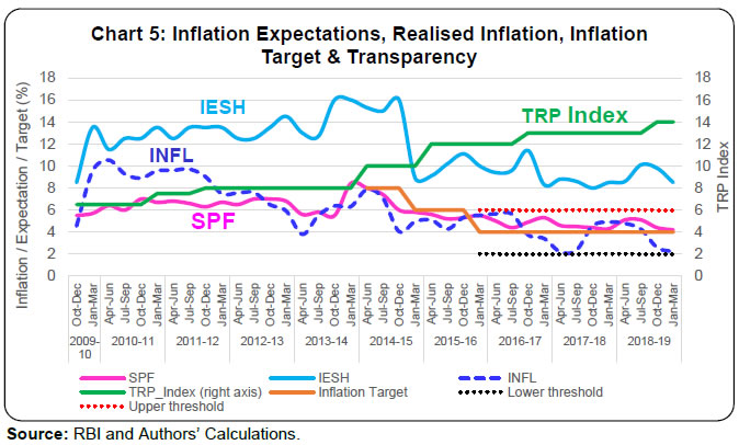 Transparency received a significant boost as soon as the announcement of adoption of the glide path of inflation was made in April 2014. The realised inflation has been within the comfort zone of the inflation target, and the expectations also appear to follow a declining path before stabilizing around new low values. Accordingly, it would be interesting to examine if transparency plays any significant role in the forming of inflation expectations. To examine how the behaviour of realised and expected inflation series evolved, we first study some basic statistics for different sub-periods. Given that RBI had announced in April 2014 a disinflationary glide path with targets of 8 per cent by end-2014, 6 per cent by end-2015 and 5 per cent by end-2016 (Patra, 2017), and also set the inflation target of 4 per cent with a variation of ±2 percentage points thereafter, and that the TRP indexes undergone a transition phase to shift from a low level to new highs during these quarters, we partition entire study period into three sub-periods/ phases or policy regimes, viz., transition-phase, pre-transition period, and post-transition period. The transition phase covers the quarters from Apr-Jun 2014 to Jul-Sep 2016. Summary statistics of inflation expectations and inflation in the three phases are provided in Table 3. Further, correlation coefficients between either of SPF and IESH expectations and realized inflation are given in Table 4. During both pre-transition and post-transition phases, inflation expectations from either SPF and IESH are much less volatile when compared with that of realised-inflation (as reflected in terms of standard deviation as well as coefficient of variation). These results indicate the possibility that during pre-and-post transition regimes, expectations didn't move as much as realised-inflation did, so the former may not be associated with the later. Indeed, correlations coefficients (Table 4) are also statistically insignificant during these periods. The IESH-based expectations, on average, are much higher as compared to both SPF-based expectations and realised-inflation. During transition-period, however, volatility (as measured by standard deviation and coefficient of variation) in actual inflation is much closer to that of survey-based expectations, indicating perhaps possible association between them. Interestingly, the correlation coefficient between SPF expectations and realized inflation is positive and statistically significant (Table 4). In the case of IESH, though the corresponding correlation is statistically insignificant, it remains positive with quite a high magnitude. | Table 3: Summary Statistics | | Period | Pre-transition
(Oct-Dec 2009 to Jan-Mar 2014) | Transition*
(Apr-Jun 2014 to Jul-Sep 2016) | Post-transition
(Oct-Dec 2016 to Jan-Mar 2019) | | Variable | SPF | IESH | INFL | SPF | IESH | INFL | SPF | IESH | INFL | | Observation | 18 | 10 | 10 | | Mean | 6.46 | 13.09 | 7.66 | 5.82 | 11.46 | 5.54 | 4.68 | 9.06 | 3.51 | | Std. Dev. | 0.72 | 1.63 | 1.98 | 1.09 | 2.82 | 1.16 | 0.39 | 1.05 | 1.10 | | Min. | 5.50 | 8.50 | 3.81 | 4.40 | 8.90 | 4.05 | 4.20 | 8.00 | 2.21 | | Max. | 8.40 | 16.00 | 10.54 | 8.00 | 16.00 | 7.86 | 5.30 | 11.40 | 4.91 | | Coefficient of variation | 0.11 | 0.12 | 0.26 | 0.19 | 0.25 | 0.21 | 0.08 | 0.12 | 0.31 |
| Table 4: Correlation Coefficient – Between Expected and Realised Inflation | | Inflation Expectation | Period/Quarters | | Pre-transition | Transition | Post-transition | Full-Sample | | SPF | 0.19 | 0.70* | 0.31 | 0.67* | | IESH | 0.01 | 0.39 | -0.01 | 0.55* | Note: '*' Significant at 5% level
Source: Authors’ Calculations. | We now move to test whether (a) expectations in pre-and-post transition periods are equal; (b) expectations during each sub-period are equal to corresponding realised inflation, and (c) the actual and expected inflation during different regimes were equal to some specified values. Empirical results of various mean equality tests are presented in Table 5. The Block/Panel A of this table presents the results of mean equality tests for SPF expectations. First, two rows in this panel show the results of two mean equality tests, viz., whether the pre-transition mean of SPF-expectations was (a) equal to 4.5 per cent, and (b) equal to mean of realized-inflation during the same period. Here negative t-statistics indicate that among two mean values under comparison, the mean of SPF-expectations was numerically lower. Similarly, the next two rows in Panel A show the results of mean equality tests for the post-transition period. Finally, the last (i.e. the fifth) row under Panel A tests whether the mean of SPF-expectations in the post-transition period was equal to that of the pre-transition period. Here, a negative value of t-statistics indicate that post-transition period mean lower than that in the pre-transition period. Same manner, Panel B and Panel C in Table 5 present the mean equality tests for IESH-expectations and realized-inflation, respectively. The results (Table 5) indicate that expectations of either professionals and households were different from inflation in both pre-and-post transition periods. Further, for the pre-transition period, the hypotheses of SPF-expectations, IESH-expectations, and realized-inflation to be equal to 6.5 per cent, 13 per cent and 7 per cent, respectively are accepted at the very high significance level (much above 10 per cent level). Whereas, in the post-transition period, the hypotheses of corresponding values to be equal to 4.5 per cent, 9 per cent and 4 per cent, respectively are accepted at a very high level of significance. Thus, results show a clear downward shift in expectations as well as actual inflation in the post-transition period. | Table 5: Mean Equality Tests | | Hypothesis tested | t statistic | p-value | Is the hypothesis accepted? (Yes/No) | | (A). Mean of SPF expectations | | Pre-transition period (Before Apr-Jun 2014) | | Equal to 6.5% | -0.2288 | 0.8218 | Yes | | Equal to inflation mean | -2.5664** | 0.0200 | No | | Post-transition period (Oct-Dec 2016 onwards) | | Equal to 4.5% | 1.4664 | 0.1766 | Yes | | Equal to inflation mean | 3.5610*** | 0.0061 | No | | Equal to pre-transition expectation mean | -8.4945*** | 0.0000 | No | | (B). Mean of IESH expectations | | Pre-transition period (Before Apr-Jun 2014) | | | | Equal to 13% | 0.2451 | 0.8093 | Yes | | Equal to inflation mean | 9.0213*** | 0.0000 | No | | Post-transition period (Oct-Dec 2016 onwards) | | | | Equal to 9% | 0.1807 | 0.8606 | Yes | | Equal to inflation mean | 11.4898*** | 0.0000 | No | | Equal to pre-transition expectation mean | -7.9316*** | 0.0000 | No | | (C). Mean of Realised-Inflation | | Pre-transition period (Before Apr-Jun 2014) | | | | Equal to 7% | 1.4068 | 0.1775 | Yes | | Post-transition period (Oct-Dec 2016 onwards) | | | | Equal to 4% | -1.4212 | 0.1890 | Yes | | Equal to pre-transition mean | -7.1390*** | 0.0000 | No | Note: '***', '**', and '*' denote significant at 1%, 5% and 10% levels, respectively.
Source: Authors’ Calculations. | Getting motivation from the empirical findings, we proceed to model the anchoring of inflation expectation as per the method described in Section IV.2. We follow the Newey-West method to adjust for the presence of auto-correlation, if any while estimating standard errors. An advantage with the Newey-West method is that it also handles the problem of heteroscedasticity of residuals if any. IV.3.2 Results for SPF expectations To estimate Eqn.(1), we need to fix a value for 'p'. In our case, at t-th quarter, we usually have inflation data upto the (t-1)th quarters, so we fix p=1. Further, considering 1-year horizon of expectations, we fix h=4. Table 6 presents estimated models, denoted by M0, M1, M2 and M3 relating to Eqn.(1). Initially, base model, denoted by M0, was estimated by regressing one-year-ahead SPF expectations on intercept and realized-inflation πt-1. Model M1 augments M0 by adding all five dummies (described in Table 2). Estimates of both the parameters in M0 are positive and statistically significant (at one per cent significance level). These results are consistent with significant positive correlation obtained for full-sample earlier (Table 4). However, given the regime changes/TRP indexes and possible change in relationship across regimes, the full-sample estimates may be inappropriate/misleading. Therefore, it would be imperative to examine whether the regression estimates are time-varying. We thus introduce dummy variables to capture possible changes in both intercept and inflation coefficient over time. Results of other models can be interpreted as discussed in Section IV. For example, Model M1 includes all five transparency dummies in the regression model. Both intercept-dummy and slope-dummy are considered. In this model, only the constant/intercept term and interaction dummy of D3 and inflation, i.e. (D3 * πt-1), appear statistically significant. It is interesting here to examine how the impact of realized-inflation (on SPF-expectation formation evolved through different regimes of policy transparency. Beginning with the insignificant value of 0.131, the coefficient of realized-inflation changes to (0.131 – 1.042) = -0.911, which is again insignificant, till the time D2 began assuming the value '1'. Before D3 starts assuming value '1', the said coefficient reduces further in magnitude to (-0.911 + 1.070) = 0.159, but thereafter the coefficient changes significantly by 0.419. Since D4 takes value '1', the coefficient of πt-1 changes further to (0.419 – 0.840) = -0.421 before becoming close to zero at (-0.421 + 0.373) = -0.048 from the quarter D5 starts assuming value '1'. Similarly, change in intercept over time can be examined from estimates of constant and coefficients of Di's , i=1,2, …, 5. | Table 6: SPF Expectations as Dependent Variable – Base Model and Other Models with Transparency Dummies | | Variable | M0 | M1 | M2 | M3 | | πt-1 | 0.302*** | 0.131 | 0.068 | 0.068 | | D1 * πt-1 | - | -1.042 | - | - | | D2 * πt-1 | - | 1.070 | - | - | | D3 * πt-1 | - | 0.419* | 0.510** | 0.590** | | D4 * πt-1 | - | -0.840 | -0.407* | - | | D5 * πt-1 | - | 0.373 | - | -0.546* | | D1 | - | 10.470 | - | - | | D2 | - | -9.961 | - | - | | D3 | - | -2.165 | -2.597* | -3.766*** | | D4 | - | 3.200 | 0.809 | - | | D5 | - | -2.253 | - | 2.116 | | Constant | 4.012*** | 4.995*** | 5.940*** | 5.940*** | | Adj. R2 | 0.431 | 0.674 | 0.684 | 0.573 | | AIC | 92.60 | 79.10 | 73.74 | 85.25 | | BIC | 95.88 | 98.75 | 83.57 | 95.07 | | DW Statistics | 0.82 | 2.21 | 1.80 | 1.34 | Note: '***', ‘**’ and ‘*’ denote significant at 1%, 5% and 10% level, respectively.
Source: Authors’ Calculations. | Among the 5 intercept-dummies, (D3 * πt-1), appears to be significant across various specifications. Further, (D4 * πt-1) or (D5 * πt-1) also turn out to be significant in some models. Therefore, we estimate model M2 which includes only the dummies D3, D4, (D3 * πt-1) and (D4 * πt-1) with base mode M0, and another model M3 that adds D3, D5, (D3 * πt-1) and (D5 * πt-1) with M0. Interestingly, while M3 uses the dummies D3 and D5, which are useful to partition our study period in pre-transition, transition, and post-transition regimes, M2 experiments with an alternative transition and post-transition periodisation. Results of these two models for SPF are broadly similar. However, to examine how the inflation expectations are anchoring changes over three policy regimes/data partition considered, we first discuss M3 in detail. The coefficient of πt-1 at 0.068 is statistically insignificant, which signifies that during the pre-transition period, SPF expectations didn't take any feedback from realized inflation. This is consistent with our earlier finding that though actual inflation did follow a declining path during these quarters, expectations hovered within a narrow band around a constant value. During the transition-phase, the impact of realized inflation on expectations was significant and positive at (0.068 + 0.590) = 0.658. This is justified by the fact that both the inflation rate and its expectations followed downward trends during this period. But in the post-transition period, the influence of inflation again faded away, as reflected in a reduction of overall impact/coefficient to only (0.658 – 0.546) = 0.112. The results are quite robust on alternative periods of transition and post-transition as reflected in model M2. Thus, it appears that the results presented here are not sensitive to identifying the transition-phase in our study period. The results of the Wald test, given in Table 7, suggest that while the combined coefficient of realised-inflation is equivalent to zero during either of pre-transition and post-transition periods, it remained significant during the transition phase. Further, the results of the Wald test are robust on the alternative selection of transition-phase (i.e. as identified either through D4 or D5). | Table 7: SPF Expectations - Regression Model and Wald Test for Significance of Combined Effect/Coefficient of πt-1 | | Variable | M2 | M3 | | Co-efficients | Wald Test | Co-efficients | Wald Test | | Hypothesis | F-Stat. | p-value | | Hypothesis | F-Stat. | p-value | | πt-1 | 0.068 | Coefficient of πt-1 = 0 | 0.88 | 0.357 | 0.068 | Coefficient of πt-1 = 0 | 0.65 | 0.427 | | D3 * πt-1 | 0.510** | Coefficients of πt-1 & (D3* πt-1) are all '0' | 8.97*** | 0.005 | 0.590** | Coefficients of πt-1 & (D3* πt-1) are all '0' | 10.96*** | 0.002 | | D4 * πt-1 | -0.407* | Coefficients of πt-1, (D3* πt-1) & (D4* πt-1) are all '0' | 1.95 | 0.172 | | - | | | | D5 * πt-1 | | - | - | - | -0.546* | Coefficients of πt-1, (D3* πt-1) & (D5* πt-1) are all '0' | 0.28 | 0.600 | | D3 | -2.597* | - | - | - | -3.766*** | - | | | | D4 | 0.809 | - | - | - | | - | | | | D5 | | - | - | - | 2.116 | - | | | | Constant | 5.940*** | - | - | - | 5.940*** | - | | | Note: '***', ‘**’ and ‘*’ denote significant at 1%, 5% and 10% level, respectively.
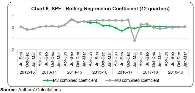
Source: Authors’ Calculations. | Thus, two institutional changes, i.e. announcement of glide path and adoption of informal inflation targeting by RBI (D3) and either the formal adoption of inflation targeting (D4) or the end-of transition phase/targeted disinflationary glide-path (D5) appear to have significant linkage with expectations, which helped to bring the survey-based inflation expectations down to respective new low levels. Notably, Cruijsen & Demertzis (2005) also find evidence of benefit from the adoption of inflation targeting in Australia and Canada. The estimates of constant/intercept term and coefficients of D3 and D5 in M3 also make some interesting findings. The estimated constant term was significant at 5.94 during the pre-transition phase when the impact of realized inflation on expectations formation was statistically insignificant. This estimated constant is very close to the average SPF-expectations observed at 6.46 during the pre-transition period. In post-transition phase, when the impact of inflation on expectations was insignificant, the overall estimate of intercept turns out to be (5.94 - 3.766 + 2.116) = 4.29, which is again very close to estimating of corresponding mean/average at 4.68. Macroeconomic disturbances may occur from time to time which may influence inflation, but the central bank does not alter its inflation target frequently. Similarly, if expectations are well anchored, respondents shall not change their expectation so often. Drawing from this analogy, in our analysis on SPF expectations, so far, we examine whether expectations are influenced by the latest realized value of inflation that was available at the time of expectations formation. However, to check the robustness further, we re-estimated the models M2 and M3 by including a few additional lags of inflation as in Eqn.(3) and check the coefficients. These extended models (given in Table 8), by-and-large, predict the evolving coefficient of πt-1 or sum of coefficients of π and its lags in line with the original models. For example, for M2, though in the variants with all 1 to 4 lags of πt-1 only the third lag appears statistically significant, the coefficient of second lag also quite substantial and opposite in sign, resulting into negligible cumulative lag-impact of πt-1 on expectations. Although the results indicate a strong linkage between realized inflation and corresponding expectation formed one year ago during transition-phase, the relationship was negligible during either of pre-and-post transition periods. However, it would be interesting to see how the relationship has evolved, i.e., whether such linkage is significant throughout the period examined. In other terms, whether the coefficient was similar in the entire period or it varied. Constrained by the non-availability of more extended time series, instead of performing separate regressions for various periods, the regression is performed on a rolling basis. Rolling regression was first carried out, keeping a window of 12 quarters at every estimation. The estimated coefficient of inflation from both the base model as well as for both M2 and M3 models are presented in Chart 6. It is clear that the coefficient of inflation was very close to zero during initial quarters, became quite large in magnitude during the transition phase, but again converged towards zero during the post-transition period. These results reconfirm the findings that while inflation expectations remained anchored in weak-form during both pre-and-post transition periods but not during the transition phase. To examine the robustness of these results, we also repeated the exercise using alternate rolling window size, viz., 8 and 16 quarters. The results for these window sizes lead to similar conclusions as obtained from 12 quarters window size (Annex II). | Table 8 – SPF Model with Additional Lags of Inflation, Eqn. (3) | | Variable | Variants of M2 | Variants of M3 | | Original Eqn. (1) | Past 4 lags of πt-1 | Select lag of πt-1 | Original Eqn. (1) | Past 4 lags of πt-1 | Select lag of πt-1 | | πt-1 | 0.068 | 0.031 | 0.072 | 0.068 | -0.030 | -0.009 | | D3 * πt-1 | 0.510** | 0.580** | 0.509** | 0.590** | 0.728*** | 0.664*** | | D4 * πt-1 | -0.407* | -0.499** | -0.409* | - | - | - | | D5 * πt-1 | - | - | | -0.546** | -0.637** | -0.512* | | πt-2 | - | 0.061 | - | - | 0.047 | - | | πt-3 | - | 0.178 | - | - | 0.290* | 0.131* | | πt-4 | - | -0.216* | 0.008 | - | -0.246 | - | | πt-5 | - | 0.084 | - | - | 0.099 | - | | D3 | -2.597* | -3.119** | -2.700* | -3.766*** | -4.501*** | -4.167*** | | D4 | 0.809 | 1.460 | 0.836 | - | - | - | | D5 | - | - | | 2.116 | 2.819** | 2.191 | | Constant | 5.940*** | 5.596*** | 5.976*** | 5.940*** | 5.382*** | 5.611*** | | Adj. R2 | 0.684 | 0.746 | 0.714 | 0.573 | 0.656 | 0.636 | | AIC | 73.74 | 65.38 | 68.15 | 85.25 | 75.68 | 77.93 | | BIC | 83.57 | 80.64 | 79.04 | 95.07 | 90.95 | 89.01 | | DW Statistics | 1.80 | 1.83 | 2.02 | 1.34 | 1.20 | 1.48 | Note: '***', ‘**’ and ‘*’ denote significant at 1%, 5% and 10% level, respectively.
Source: Authors’ Calculations. |
 IV.3.3 Results for IESH expectations Summary results of the base model (M0) and models augmented with transparency dummies about IESH expectations are given in Table 9. The base model without any dummy reveals that the coefficient of inflation in Eqn. (1) would be positive and statistically significant, and so is also reflected in the significant positive correlation between realised and expected inflation, when estimates are based on full-sample data (Table 4). However, like the case of SPF expectations, here also the full-sample estimates may not give reliable picture given that full-data period consists of multiple transparency/policy regimes, viz., pre-transition, transition and post-transition periods. Like earlier, when we augment the base model with transparency dummies – both for intercept and interaction with inflation – the effective impact of inflation shows changing pattern. The model M1, which extends the base model by including all dummies shows that coefficients of all intercept and interaction dummies are insignificant, though the magnitude of some of them appears high. The models M2 and M3 are of interest as either of them use two transparency dummies, either {D3, D4} or {D3, D5} aligned with alternative partitioning of study period into pre-transition, transition and post-transition periods. Results are broadly similar in line with those obtained for SPF. It is seen that irrespective of partitioning considered, the households' expectations did not take feedback from realised-inflation during both pre-and-post transition periods. Once again, like the case of SPF, IESH expectations declined in association with actual inflation during the transition phase. Further, the Wald tests (Table 10) reconfirmed that on cumulative-basis, while the overall impact of inflation in M2 and M3 during both pre-and-post transition periods was insignificant, the same was significant during the transition period, albeit at 10 per cent level. This is observed more clearly when we carry out rolling regression (Chart 7 & Annex II). | Table 9: IESH Expectations as the Dependent Variable – Base Model and Other Models with Transparency Dummies | | Variable | M0 | M1 | M2 | M3 | | πt-1 | 0.592*** | 0.698** | 0.006 | 0.006 | | D1 * πt-1 | - | 1.205 | - | - | | D2 * πt-1 | - | -1.995 | - | - | | D3 * πt-1 | - | 0.613 | 0.515 | 0.934 | | D4 * πt-1 | - | -0.778 | -0.309 | - | | D5 * πt-1 | - | 0.243 | - | -0.954 | | D1 | - | -10.870 | - | - | | D2 | - | 19.530 | - | - | | D3 | - | -3.697 | -2.365 | -6.801* | | D4 | - | 0.565 | -2.189 | - | | D5 | - | -2.140 | - | 2.860 | | Constant | 8.047*** | 5.717* | 13.047*** | 13.050*** | | Adj. R2 | 0.287 | 0.615 | 0.554 | 0.420 | | AIC | 166.6 | 150.9 | 152.4 | 162.3 | | BIC | 169.9 | 170.5 | 162.2 | 172.1 | | DW Statistics | 0.82 | 2.16 | 1.76 | 1.44 | Note: '***', ‘**’ and ‘*’ denote significant at 1%, 5% and 10% level, respectively.
Source: Authors’ Calculations. |
| Table 10: IESH Expectations – Regression Model and Wald Test for Significance of Combined Effect/Coefficient of πt-1 | | Variable | M2 | M3 | | Coefficients | Wald Test | | Wald Test | | | Hypothesis | F-Stat. | p-value | Coefficients | Hypothesis | F-Stat. | p-value | | πt-1 | 0.006 | Coefficient of πt-1 = 0 | 0.00 | 0.976 | Coefficient of πt-1 = 0 | 0.006 | 0.00 | 0.979 | | D3 * πt-1 | 0.515 | Coefficients of πt-1 & (D3* πt-1) are all '0' | 0.92 | 0.344 | Coefficients of πt-1 & (D3* πt-1) are all '0' | 0.934 | 2.95* | 0.095 | | D4 * πt-1 | -0.309 | Coefficients of πt-1, (D3* πt-1) & (D4* πt-1) are all '0' | 0.38 | 0.542 | - | - | - | - | | D5 * πt-1 | - | - | - | - | Coefficients of πt-1, (D3* πt-1) & (D5* πt-1) are all '0' | -0.954 | 0.00 | 0.982 | | D3 | -2.365 | - | - | - | - | -6.801* | - | - | | D4 | -2.189 | - | - | - | - | - | - | - | | D5 | - | - | - | - | - | 2.860 | - | - | | Constant | 13.047*** | - | - | - | - | 13.050*** | - | - | Note: '***', ‘**’ and ‘*’ denote significant at 1%, 5% and 10% level, respectively.
Source: Authors’ Calculations. | Rolling regression results (Chart 7 for window size 12 quarters, and Annex II for window size 8 and 16 quarters) also confirm the results. Further, to check the robustness, we include a few additional lags from 1 to 4 of πt-1 and check the coefficients (Eqn. 3). Results, presented in Table 11, reveal the conclusion similar to what we saw for corresponding models under Eqn.1. 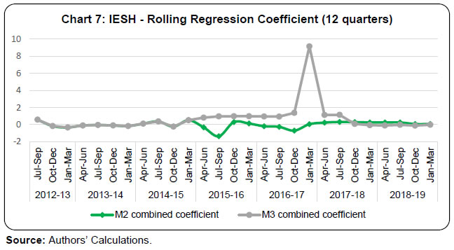
| Table 11 – IESH Model with Additional Lags of Inflation, Eqn. (3) | | Variable | Variants of M2 | Variants of M3 | | Original Eqn. (1) | Past 4 lags of πt-1 | Select lag of πt-1 | Original Eqn. (1) | Past 4 lags of πt-1 | Select lag of πt-1 | | πt-1 | 0.006 | -0.528* | -0.466* | 0.006 | -0.720* | -0.546* | | D3 * πt-1 | 0.515 | 0.558 | 0.909* | 0.934 | 1.211* | 1.320** | | D4 * πt-1 | -0.309 | -0.394 | -0.408 | - | - | - | | D5 * πt-1 | - | - | - | -0.954 | -1.343* | -0.995 | | πt-2 | - | 0.931** | 0.289 | - | 0.903** | 0.401* | | πt-3 | - | -0.305 | - | - | 0.061 | - | | πt-4 | - | -0.316 | - | - | -0.388 | - | | πt-5 | - | -0.034 | - | - | -0.094 | - | | D3 | -2.365 | -3.578 | -5.463 | -6.801* | -9.435** | -9.626*** | | D4 | -2.189 | -2.262 | -1.345 | - | - | - | | D5 | - | - | | 2.860 | 4.342 | 3.372 | | Constant | 13.047*** | 15.666*** | 14.787*** | 13.050*** | 15.480*** | 14.550*** | | Adj. R2 | 0.554 | 0.760 | 0.682 | 0.420 | 0.617 | 0.562 | | AIC | 152.4 | 120.3 | 136.1 | 162.3 | 136.2 | 148.0 | | BIC | 162.2 | 135.6 | 147.4 | 172.1 | 151.4 | 159.3 | | DW | 1.76 | 2.05 | 1.97 | 1.44 | 1.56 | 1.51 | Note: '***', ‘**’ and ‘*’ denote significant at 1%, 5% and 10% level, respectively.
Source: Authors’ Calculations. | V. Conclusion The central banks across the countries have attached increasing importance in recent decades to both monetary policy transparency and anchoring of private agents' inflation expectations. However, precise measurement of transparency is difficult, and the literature provides multiple measures of transparency. A credible central bank can use communication as a useful tool to influence/manage market expectations and thereby policy transmission. However, like transparency, anchoring is also defined in multiple ways, and empirical literature provides mixed results on both degrees of anchoring and its role in monetary policy. Further, anchoring varies over time, respondent categories, and economic sectors as well as across countries and over policy regimes. Against the above backdrop, this paper has two broad objectives: (a) construct an index to measure the evolving monetary policy transparency in India since 2009, and (b) assess whether and how far the one-year-ahead inflation expectations of households and professionals, captured through two RBI surveys, viz., SPF and IESH, have been anchored. We determine transparency based on publications and information disseminated by RBI and the construction of transparency index was aided by text-mining approach. As seen in earlier studies, the transparency index exhibits a step-like pattern. It is found that, as India moved towards an inflation targeting regime, the degree of transparency enhanced greatly. Based on the timing and magnitude of changes in the transparency index, we identify that our study period consists of three distinct transparency/policy regimes: transition, pre-transition and post-transition periods. Interestingly, these transition phases broadly coincide with the periods of RBI's adoption of self-imposed disinflationary glide path since 2014 and implementation of flexible inflation targeting in 2016. Starting from a low value before 2014, transparency index increased substantially on two occasions during the policy transition period, and during the post-transition period, the degree of transparency continued to remain high and stable. As regards inflation expectations anchoring, we follow the stream of literature which defines expectations anchoring in terms of the relationship between survey-based expectations and available set of information at the time of expectation formation. Depending on the underlying information base, the expectations anchoring aspect has been categorised into three types, viz., weak-form, semi-strong-form and strong-form. Empirical analysis on weak-form suggests that the participants of SPF could anchor their inflation expectations slightly above the central value of inflation target post-adoption of the FIT framework by the RBI and policy transparency index improved substantially during this period. Households' inflation expectations were also found to be anchored in weak-form during this period, as they do not appear to be influenced by realised inflation, though the anchoring point remains above the upper limit/band of the RBI's inflation target. Further, during the pre-transition period, expectations of both households and professionals were reasonably anchored in weak-form, albeit at a higher level, when compared with the post-transition period. During this period though actual inflation declined gradually, neither professionals nor the households appear to have taken feedback from falling inflation to form their expectations. Interestingly, during the transition phase, when transparency improved substantially on a few occasions, both the realised and expected inflation declined in tandem resulting in a case of no anchoring of inflation expectations. The present study focuses on the weak-form of inflation expectations anchoring. Future research may extend this work in many ways. One straightforward application would involve the investigation of semi-strong/strong or other types of expectations anchoring defined in the literature, such as ideally anchored, consistently anchored, and so on. It would be of interest to examine the potential benefits of anchoring – through wage-price dynamics – and its role under variants of Phillips-curves or output-gap models. Further, one may look at the consequences and effects of policy transparency on lags and magnitude of policy transmission.
References Benes, J., Clinton, K., George, A. T., Gupta, P., John, J., Kamenik, O., Laxton, D., Mitra, P., Nadhanael, G. V., Portillo, R., Wang, H., & Zhang, F. (2016). Quarterly Projection Model for India: Key Elements and Properties. RBI Working Paper No. 8. Bini-Smaghi, L. & Gros, D. (2001). Is The ECB Sufficiently Accountable and Transparent?. ENEPRI Working Paper No. 7. Blinder, A. S. (2002). Through the looking glass: Central Bank Transparency. CEPS Working Paper No. 86. Blinder, A. S., Ehrmann, M., Fratzscher, M., De Haan, J. & Jansen, D.J (2008). Central Bank Communication and Monetary Policy: A Survey of Theory and Evidence. NBER Working Paper No. 13932. Bordoloi, S., Kavedia, R., Roy, S. & Goyal, A. (2019). Changes in Macroeconomic Perceptions: Evidence from the Survey of Professional Forecasters. RBI Bulletin November, 15-26. Carvalho, C., Eusepi, S., Moench, E. & Preston, B. (2017). Anchored Inflation Expectations. (Available at SSRN: https://ssrn.com/abstract=3018198 or http://dx.doi.org/10.2139/ssrn.3018198; downloaded on July 14, 2019). Choi, S., Furceri, D. & Loungani, P. (2018). Inflation Anchoring and Growth: Evidence from Sectoral Data. IMF Working Paper No. 18/36. Cruijsen, C. van der & Demertzis, M. (2005). The Impact of Central Bank Transparency on Inflation Expectations. DNB Working Paper No. 31. Demertzis, M. & Hallet, A. H. (2007). Central Bank Transparency in Theory and Practice. Journal of Macroeconomics, 29, 760-789. Dincer, N. N. & Eichengreen, B. (2014). Central Bank Transparency and Independence: Updates and New Measures. International Journal of Central Banking, 10, 189-253. Eijffinger, S. C. W. & Geraats, P. M. (2006). How Transparent Are Central Banks. European Journal of Political Economy, 22, 1-21. Fama, E. F. (1970). Efficient Capital Markets: A Review of Theory and Empirical Work. The Journal of Finance, 25(2), 383-417. Fama, E. F. (1991). Efficient Capital Markets: II. The Journal of Finance, 46(5), 1575-1617. Geraats, P. M. (2002). Central Bank Transparency. The Economic Journal, 112(483), F532-F565. Geraats, P. M. (2009). Trends in Monetary Policy Transparency. CESifo Working Paper No. 2584. Hubert, P. (2015). ECB Projections as a Tool for Understanding Policy Decisions. Journal of Forecasting, 34(7), 574-587. Kedan, D. & Stuart, R. (2014). Central Bank Communications: A Comparative Study. Central Bank of Ireland Quarterly Bulletin 02, 89-104. Kumar, S., Afrouzi, H., Coibion, O. & Gorodnichenko, Y. (2015). Inflation Targeting Does Not Anchor Inflation Expectations: Evidence from Firms in New Zealand. Brookings Paper on Economic Activity, Fall. Levin, A. T., Natalucci, F. M. & Piger, J. M. (2004). The Macroeconomic Effects of Inflation Targeting. Federal Reserve Bank of St. Louis Review, 86(4), 51-80. Liikanen, E. (2017). Is More Always Better? Transparency, Accountability, and the Clarity of Message. ECB Central Bank Communications Conference. Lyziak, T. & Paloviita, M. (2016). Anchoring of Inflation Expectations in the Euro Area: Recent Evidence Based on Survey Data. ECB Working Paper No. 1945. Mohan, R. (2009). Communications in Central Banks: A Perspective. Stanford Centre for International Development Working Paper No. 408. Oikonomou, G. & Spyromitros, E. (2017). Trends in Central Bank Transparency. Theoretical Economics Letters, 7, 2089-2103. Patra, M. D. & Ray, P. (2010). Inflation Expectations and Monetary Policy in India: An Empirical Exploration. IMF Working Paper No. 10/84. Patra, M. D. (2017). One Year in the Life of India's Monetary Policy Committee. Speech delivered at the Jaipur Regional Office of the RBI on October 27, 2017. (https://www.rbi.org.in/Scripts/BS_SpeechesView.aspx?Id=1050). Rajan, R. (2013). Statement by Dr. Raghuram Rajan on taking office on September 4, 2013.https://www.rbi.org.in/scripts/BS_PressReleaseDisplay.aspx?prid=29479). RBI (2010). Inflation Expectations Survey of Households. RBI Bulletin May, 1161-1226. RBI (2013). Survey of Professional Forecasters. RBI Bulletin December, 73-82. RBI (2014). Report of the Expert Committee to Revise and Strengthen the Monetary Policy Framework (Chairman: Dr. Urjit R. Patel). RBI (2017). Inflation Expectations Survey of Households, 2016-17. RBI Bulletin June, 41-48. Sousa, R. & Yetman, J. (2016). Inflation Expectations and Monetary Policy. BIS Papers No. 89 Subbarao, D. (2011). Dilemmas in Central Bank Communication - Some Reflections Based on Recent Experience. Second Business Standard Annual Lecture, New Delhi, January. Warsh, K. (2014). Transparency and the Bank of England's Monetary Policy Committee. (https://www.hoover.org/sites/default/files/transparency_and_the_bank_of_englands_monetary_policy_committee.pdf ; Downloaded: May 2020).
Annex I: Monetary Policy Transparency (TRP) Index In this Annex, we first present the estimated four variants of TRP index, viz., V1, V2, V3 and V4 for October 2009, which is the first month of the study period (Table I.1), followed by incremental change post-October 2009 (Table I.2). The TRP index is the sum of scores for the answers to the fifteen questions below (minimum score=0, maximum score=1515). Reasons for differences in scores for V2, V3 and V4 from V1 are as below; -
V2 - This variant assumes that consistent time-series data on unemployment is not available (Q2.1). -
V3 - This variant considers the MPFA executed in 2015, which paved the way for FIT, as earlier framework existed without any specific quantified target (Q3.1). -
V4 - This variant takes into account that explicit future policy inclination is not provided after every policy meeting (Q4.3). | Table I.1: Score in October 2009 | | # | Category / Question | V1 | V2 | V3 | V4 | | 1 | Mandate / Political transparency | 0 | 0 | 0 | 0 | | (1) | Formal objective | 0 | 0 | 0 | 0 | | (2) | Quantification of objective | 0 | 0 | 0 | 0 | | (3) | Institutional arrangement between Govt. and central bank | 0 | 0 | 0 | 0 | | 2 | Economic transparency | 1.5 | 1.5 | 1.5 | 1.5 | | (1) | Availability of relevant data for policy-making | 0.5 | 0.5 | 0.5 | 0.5 | | (2) | Publication of internal models | 0 | 0 | 0 | 0 | | (3) | Publication of macroeconomic forecasts | 1 | 1 | 1 | 1 | | 3 | Procedural transparency | 1 | 1 | 0 | 1 | | (1) | Policy strategy describing monetary policy framework | 1 | 1 | 0 | 1 | | (2) | Publication of deliberations/ MPC meeting minutes | 0 | 0 | 0 | 0 | | (3) | Publication of voting records | 0 | 0 | 0 | 0 | | 4 | Policy (communication) transparency | 3 | 3 | 3 | 2 | | (1) | Prompt announcement of policy decisions | 1 | 1 | 1 | 1 | | (2) | Rationale behind the decisions | 1 | 1 | 1 | 1 | | (3) | Indication of likely future actions | 1 | 1 | 1 | 0 | | 5 | Operational transparency | 1 | 1 | 1 | 1 | | (1) | Evaluation of target achievement | 1 | 1 | 1 | 1 | | (2) | Evaluation of transmission process | 0 | 0 | 0 | 0 | | (3) | Evaluation of policy outcome | 0 | 0 | 0 | 0 | | | TRP Index (aggregated score) | 6.5 | 6.5 | 5.5 | 5.5 |
| Table I.2: Incremental change in transparency | | Month of change | V1 | V2 | V3 | V4 | | January 2011 | (1, 7.5)
[Procedural transparency Q3.2 score increased from 0 to 1 - TACMP minutes publication started] | (1, 7.5)
[same as V1] | (1, 6.5)
[same as V1] | (1, 6.5)
[same as V1] | | October 2011 | (0.5, 8)
[Economic transparency Q2.1 score increased from 0.5 to 1 - CU publication started along with survey results] | (0, 7.5)
[this variant assumes that consistent time-series data on unemployment is not available and therefore CU publication did not alter the score of Q2.1] | (0.5, 7)
[same as V1] | (0.5, 7)
[same as V1] | | April 2014 | (2, 10)
[Political transparency Q1.1 and Q1.2 score increased from 0 to 1 – disinflationary glide path announcement, self-imposed targets] | (2, 9.5)
[same as V1] | (2, 9)
[same as V1] | (2, 9)
[same as V1] | | April 2015 | (2, 12)
[Political transparency Q1.3 score increased from 0 to 1 – first monetary policy after MPFA for FIT came into place; Operational transparency Q5.2 and Q5.3 score improved from 0 to 0.5 - MPR publication giving more details including forecast errors started] | (2, 11.5)
[same as V1] | (3, 12)
[same as V1 + Q3.1 score improved from 0 to 1 - Revised framework with targets and strategy came into existence] | (2, 11)
[same as V1] | | October 2016 | (1, 13)
[Procedural transparency Q3.3 score improved from 0 to 1 - MPC meeting minutes publication started with individual votes] | (1, 12.5)
[same as V1] | (1, 13)
[same as V1] | (1, 12)
[same as V1] | | October 2018 | (1, 14)
[Economic transparency Q2.2 score improved from 0 to 1 - explicit reference of model used in policy analysis is provided in MPR] | (1, 13.5)
[same as V1] | (1, 14)
[same as V1] | (1, 13)
[same as V1] | | Note: First number in ( ) represents incremental score at the corresponding month and second number represents overall / cumulative score upto the same month. Text in [ ] represents the reason of increment in transparency score. | Annex II: Rolling Regression Results II.1 Rolling Regression Results – SPF
II.2 Rolling Regression Results – IESH
|