1. Introduction 2.1 This chapter analyses the consolidated finances of states reflected in their budgets for 2020-21, with the caveat that most states released their budgets in February-March 2020, i.e., prior to the outbreak of COVID-19 in India1. Hence, budget estimates (BE) are likely to get substantially revised. Nonetheless, the analysis assumes significance as an early warning sensor, as the states are in the vanguard of the fight against the pandemic. As is widely anticipated, the COVID-19-related lockdown and containment measures may impact states’ revenue coincident with higher expenditure to manage the health crisis and heal and restore economic activity to pre-COVID-19 levels. 2.2 The rest of this chapter is divided into seven sections. Against the backdrop of an overview of key fiscal parameters in Section 2, the chapter examines actual budgetary outcomes for 2018-19, revised estimates (RE) for 2019-20 and BE for 2020-21 in Sections 3, 4 and 5, respectively. Section 5 also throws light on specific COVID-19 effects on expected fiscal outcomes during 2020-21 that have macro-economic and financial implications. Section 6 deals with the financing pattern of states’ combined gross fiscal deficit and Section 7 addresses outstanding liabilities of states, including contingent liabilities. Section 8 sets out concluding observations. 2. Key Fiscal Indicators 2.3 States have budgeted their consolidated gross fiscal deficit (GFD) at 2.8 per cent of GDP in 2020-21. Although the RE for 2019-20 placed the GFD at 3.2 per cent of GDP (Table II.1), provisional accounts released by the Office of the Comptroller and Auditor General (CAG) of India indicate that the budgeted level was achieved through large cutbacks on both revenue and capital expenditure to compensate for cyclical shortfalls in tax collections (Box II.1). | Table II.1: Major Deficit Indicators - All States and Union Territories with Legislature | | (₹ lakh crore) | | Item | 2006-11 (Average) | 2011-16 (Average) | 2016-17 | 2017-18 | 2018-19 | 2019-20 (BE) | 2019-20 (RE) | 2020-21 (BE) | | 1 | 2 | 3 | 4 | 5 | 6 | 7 | 8 | 9 | | Gross Fiscal Deficit | 1.30 | 2.74 | 5.36 | 4.10 | 4.63 | 5.54 | 6.52 | 6.26 | | (Per cent of GDP) | (2.2) | (2.4) | (3.5) | (2.4) | (2.4) | (2.6) | (3.2) | (2.8) | | Revenue Deficit | -0.17 | -0.02 | 0.36 | 0.19 | 0.18 | -0.08 | 1.37 | 0.00 | | (Per cent of GDP) | (-0.4) | (-0.0) | (0.2) | (0.1) | (0.1) | (-0.0) | (0.7) | (0.0) | | Primary Deficit | 0.20 | 0.98 | 2.81 | 1.17 | 1.44 | 1.99 | 3.04 | 2.38 | | (Per cent of GDP) | (0.3) | (0.8) | (1.8) | (0.7) | (0.8) | (0.9) | (1.5) | (1.1) | BE: Budget Estimates. RE: Revised Estimates.
Notes: 1. Data include 31 states and union territories with legislature.
2. Negative (-) sign indicates surplus.
3. GDP at current market prices is based on the National Statistical Office (NSO)’s National Accounts 2011-12 series.
Source: Budget documents of state governments. |
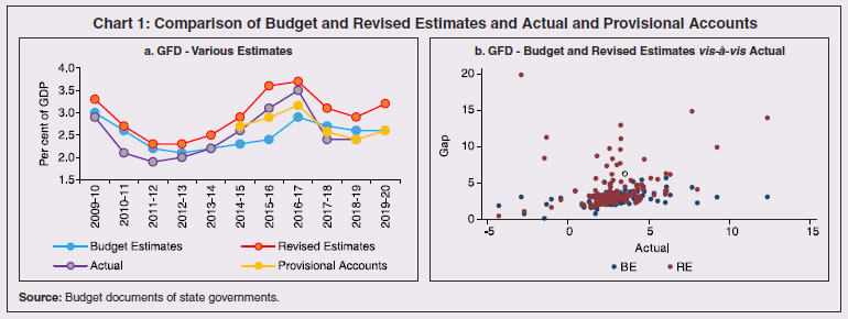
Box II.1: Is there a Systematic Bias in Revised Estimates? The aggregation of monthly provisional accounts (PA) estimates of states’ receipts and expenditure by the Comptroller and Auditor General of India (CAG) for individual states is a timely indicator for assessing the true fiscal position of states, albeit at the cost of loss of some granularity. For every fiscal year, budget estimates (BE) give a projection before the start of the year, while revised estimates (RE) are available towards the end of the fiscal year. PA are available with a lag of about another two months, and accounts arrive with an additional lag of about nine to ten months. RE reveal a systematic upward bias, albeit with outliers across states (Chart 1a and 1b). The Reserve Bank of India started consolidating monthly PA data across states for 2018-19 and released them along with RE in the State Finances: A Study of Budgets of 2019-20. 2019-20 PA indicate that the GFD-GDP ratio was 2.6 per cent, exactly as budgeted, as against RE of 3.2 per cent (Table 1). In a panel framework for 24 states for the period 2014-15 to 2019-20 using three gap variables – Gap1 (difference between actual and BE), Gap2 (difference between actual and RE) and Gap3 (difference between actual and PA), a test is conducted to check if the means of these gap variables are statistically different from zero. A simple fixed effects model without any explanatory variables is estimated using equation (1) to examine if the intercept term is statistically close to zero, and standard t-tests reported below (Table 2). | Table 1: Fiscal Position of States | | (₹ lakh crore) | | | 2017-18 | 2018-19 | 2019-20 BE | 2019-20 RE | 2019-20 PA | 2020-21 BE | | I. Revenue Receipts | 23.21 | 26.21 | 31.54 | 29.40 | 27.63 | 33.27 | | | (13.6) | (13.8) | (14.9) | (14.5) | (13.6) | (14.8) | | II. Capital Receipts | 0.40 | 0.41 | 0.62 | 0.60 | 0.45 | 0.16 | | | (0.2) | (0.2) | (0.3) | (0.3) | (0.2) | (0.1) | | III. Revenue Expenditure | 23.40 | 26.38 | 31.46 | 31.76 | 28.36 | 33.27 | | | (13.7) | (13.9) | (14.9) | (15.1) | (13.9) | (14.8) | | IV. Capital Expenditure | 4.31 | 4.87 | 6.22 | 5.78 | 4.97 | 6.46 | | | (2.5) | (2.6) | (2.9) | (2.8) | (2.4) | (2.9) | | a. Capital Outlay | 3.94 | 4.40 | 5.81 | 5.31 | 4.55 | 5.98 | | | (2.3) | (2.3) | (2.8) | (2.6) | (2.2) | (2.7) | | b. Loans and Advances by States | 0.38 | 0.47 | 0.41 | 0.47 | 0.42 | 0.48 | | | (0.2) | (0.3) | (0.1) | (0.2) | (0.2) | (0.2) | | V. Fiscal Deficit/Surplus | 4.10 | 4.63 | 5.54 | 6.52 | 5.25 | 6.26 | | | (2.4) | (2.4) | (2.6) | (3.2) | (2.6) | (2.8) | | VI. Revenue Deficit/Surplus | 0.19 | 0.18 | -0.08 | 1.37 | 0.72 | 0.00 | | | (0.1) | (0.1) | (-0.0) | (0.7) | (0.4) | (0.0) | Note: (1) Figures in parentheses are per cent of GDP.
(2) Data for 2019-20 Provisional Accounts (PA) are accounts figures of 24 states available with CAG and for the remaining 7 states/UTs 2019-20 Budget Estimates (BE) figures are used to arrive at all states and UTs.
Sources: Budget documents of state governments and CAG. |
| Table 2: Panel Fixed Effect Model of Gap Variables | | Dependent Variable# | Intercept | Std. Error | t-statistics | p-value | Remark | | Gap1 | 0.059 | 0.158 | 0.37 | 0.710 | Mean is same | | Gap2 | -1.193 | 0.305 | -3.91 | 0.000** | Mean is different | | Gap3 | -0.016 | 0.103 | -0.16 | 0.877 | Mean is same | # Gap between actual and other estimates - BE, RE and PA.
** Significance at 5 per cent level of significance.
Source: RBI staff estimates. |
 The results show that the average gap of BE and PA from actuals is not statistically different from zero, with the means across states being almost equal, while the deviation of RE from actual is statistically significant. The negative and statistically significant sign for Gap2 indicates an upward bias in RE. These results have two important policy implications. First, PA consolidated across states can be safely used as a benchmark for making comparative assessments of fiscal performance across time for policy purposes instead of the RE. Second, considering that the 2020-21 BE is projected with 2019-20 RE as the base, the large shortfall in receipts in 2019-20 PA vis-à-vis the RE clearly distorts the fiscal arithmetic for 2020-21 BE, even without the impact of the pandemic. | 2.4 In the event, these movements in states’ finances have possibly negated the fiscal impulse from central finances in that year to counter the cyclical slowdown. Cuts in spending also explain the improvement in 2018-19 (Table II.1 and Chart II.1). 2.5 In 2020-21, about half of the states have budgeted the GFD-GSDP ratio at or above the 3 per cent threshold although, as stated earlier, most of these budgets were presented prior to the onset of COVID-19 (Chart II.2). The direction of possible revision is evident from the fact that the average for states presenting their budget before the outbreak of the pandemic is 2.4 per cent, while the average for the balance number of states that made post-outbreak budget presentation is 4.6 per cent of GSDP. 2.6 Thus, states are grappling with the pandemic with constrained fiscal space. In terms of primary balances, states are clearly in an unfavourable position, with most states incurring primary deficits in 2019-20, as against primary surpluses at the onset of the global financial crisis (Chart II.3).
3. 2018-19: Accounts 2.7 For the second consecutive year, states maintained their GFD at 2.4 per cent of GDP in 2018-19 (Chart II.4). This rectitude was brought about by higher revenue receipts on account of tax devolution, even though revenue expenditure and capital expenditure increased (Table II.2). 2.8 The tax revenue to GDP ratio increased marginally with the higher devolution, partly offset by lower own tax revenue (Table II.2), although the latter was made good through the GST compensation cess, booked as grant-in-aid from the centre in accounting terms. Lower own tax revenue was reflected in a sharp decline in sales tax/value added tax (VAT), even as states’ goods and services tax (SGST) collections increased.
2.9 Non-tax revenue, comprising own non-tax revenue and grants from the centre improved in 2018-19 vis-à-vis 2017-18, driven by higher collections from general services and petroleum (Table II.2).2.10 The rise in revenue expenditure in 2018-19 vis-à-vis the preceding year was largely on the non-developmental front (Table II.3). Appropriation for reduction or avoidance of debt increased along with other committed expenditures like pensions and administrative and miscellaneous general services. | Table II.2: Aggregate Receipts of State Governments and UTs | | (₹ lakh crore) | | Item | 2016-17 | 2017-18 | 2018-19 | 2019-20 (RE) | 2020-21 (BE) | | 1 | 2 | 3 | 4 | 5 | 6 | | Aggregate Receipts (1+2) | 26.46 | 27.76 | 31.27 | 35.90 | 39.53 | | | (17.3) | (16.2) | (16.5) | (17.6) | (17.6) | | 1. Revenue Receipts (a+b) | 20.81 | 23.21 | 26.20 | 29.40 | 33.27 | | | (13.6) | (13.6) | (13.8) | (14.5) | (14.8) | | a. States' Own Revenue (i+ii) | 11.17 | 13.10 | 14.34 | 15.79 | 17.66 | | | (7.3) | (7.7) | (7.6) | (7.8) | (7.9) | | i. States' Own Tax | 9.46 | 11.30 | 12.15 | 13.40 | 14.98 | | | (6.1) | (6.6) | (6.4) | (6.6) | (6.7) | | ii. States' Own Non-Tax | 1.71 | 1.80 | 2.19 | 2.39 | 2.68 | | | (1.1) | (1.1) | (1.2) | (1.2) | (1.2) | | b. Central Transfers (i+ii) | 9.69 | 10.11 | 11.87 | 13.60 | 15.60 | | | (6.3) | (5.9) | (6.3) | (6.7) | (6.9) | | i. Shareable Taxes | 6.08 | 6.05 | 7.47 | 7.03 | 8.17 | | | (3.9) | (3.5) | (3.9) | (3.5) | (3.6) | | ii. Grants-in Aid | 3.61 | 4.06 | 4.40 | 6.57 | 7.43 | | | (2.3) | (2.4) | (2.3) | (3.2) | (3.3) | | 2. Net Capital Receipts (a+b) | 5.61 | 4.54 | 5.06 | 6.50 | 6.26 | | | (3.3) | (2.7) | (2.7) | (3.2) | (2.8) | | a. Non-Debt Capital Receipts (i+ii) | 0.16 | 0.40 | 0.42 | 0.62 | 0.20 | | | (0.1) | (0.2) | (0.2) | (0.3) | (0.1) | | i. Recovery of Loans and Advances | 0.16 | 0.40 | 0.41 | 0.60 | 0.16 | | | (0.1) | (0.2) | (0.2) | (0.3) | (0.1) | | ii. Miscellaneous Capital Receipts | 0.00 | 0.00 | 0.01 | 0.02 | 0.04 | | | (0.0) | (0.0) | (0.0) | (0.0) | (0.0) | | b. Debt Receipts (i+ii) | 5.45 | 4.15 | 4.64 | 5.88 | 6.06 | | | (3.6) | (2.4) | (2.4) | (2.9) | (2.7) | | i. Market Borrowings | 3.52 | 3.45 | 3.73 | 4.88 | 5.61 | | | (2.3) | (2.0) | (2.0) | (2.4) | (2.5) | | ii. Other Debt Receipts | 1.93 | 0.70 | 0.91 | 1.00 | 0.45 | | | (1.3) | (0.4) | (0.5) | (0.5) | (0.2) | RE: Revised Estimates. BE: Budget Estimates.
Notes: 1. Figures in parentheses are per cent of GDP.
2. Debt receipts are on net basis.
Source: Budget documents of state governments. |
| Table II.3: Revenue Expenditure Pattern of State Governments and UTs | | (₹ lakh crore) | | Item | 2016-17 | 2017-18 | 2018-19 | 2019-20 (RE) | 2020-21 (BE) | | 1 | 2 | 3 | 4 | 5 | 6 | | Revenue Expenditure (1+2) | 21.22 | 23.40 | 26.38 | 30.76 | 33.27 | | | (13.8) | (13.7) | (13.9) | (15.1) | (14.8) | | 1. Development Expenditure (i+ii) | 13.66 | 14.66 | 16.36 | 19.46 | 20.68 | | | (8.9) | (8.6) | (8.6) | (9.6) | (9.2) | | (i) Social Services | 8.54 | 9.13 | 10.32 | 12.24 | 13.35 | | | (5.5) | (5.3) | (5.4) | (6.0) | (5.9) | | (ii) Economic Services | 5.12 | 5.53 | 6.04 | 7.23 | 7.32 | | | (3.3) | (3.2) | (3.2) | (3.6) | (3.3) | | 2. Non-development Expenditure | 6.99 | 8.06 | 9.22 | 10.36 | 11.64 | | of which: | (4.5) | (4.7) | (4.9) | (5.1) | (5.2) | | Appropriation for Reduction or Avoidance of Debt | 0.16 | 0.18 | 0.34 | 0.21 | 0.39 | | | (0.1) | (0.1) | (0.2) | (0.1) | (0.2) | | Interest Payments | 2.55 | 2.93 | 3.19 | 3.49 | 3.89 | | | (1.7) | (1.7) | (1.7) | (1.7) | (1.7) | | Pension | 2.27 | 2.75 | 3.15 | 3.55 | 3.86 | | | (1.5) | (1.6) | (1.7) | (1.7) | (1.7) | | Administrative Services | 1.47 | 1.62 | 1.84 | 2.20 | 2.56 | | | (1.0) | (0.9) | (1.0) | (1.1) | (1.1) | RE: Revised Estimates. BE: Budget Estimates.
Note: Figures in parentheses are per cent of GDP.
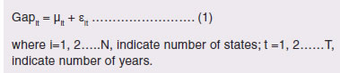
Source: Budget documents of state governments. | 2.11 Under developmental expenditure, there were reallocations under social and economic services (Chart II.5). 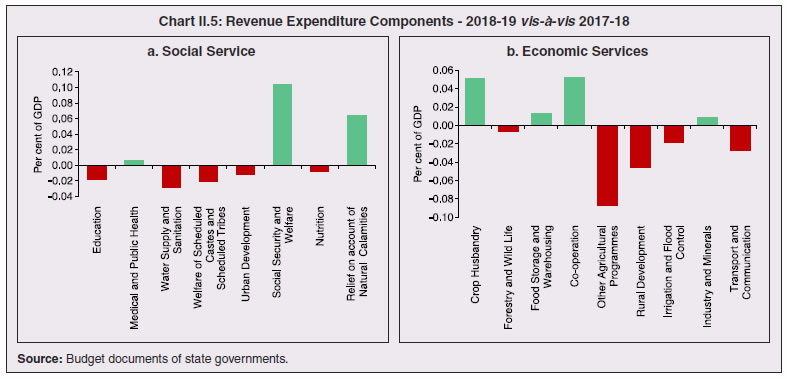
| Table II.4: Expenditure Pattern of State Governments and UTs | | (₹ lakh crore) | | Item | 2016-17 | 2017-18 | 2018-19 | 2019-20 (RE) | 2020-21 (BE) | | 1 | 2 | 3 | 4 | 5 | 6 | | Aggregate Expenditure (1+2 = 3+4+5) | 26.38 | 27.72 | 31.25 | 36.54 | 39.73 | | | (17.1) | (16.2) | (16.5) | (18.0) | (17.7) | | 1. Revenue Expenditure | 21.22 | 23.40 | 26.38 | 30.76 | 33.27 | | of which: | (13.8) | (13.7) | (13.9) | (15.1) | (14.8) | | Interest payments | 2.55 | 2.93 | 3.19 | 3.49 | 3.89 | | | (1.7) | (1.7) | (1.7) | (1.7) | (1.7) | | 2. Capital Expenditure | 5.17 | 4.31 | 4.87 | 5.78 | 6.46 | | of which: | (3.4) | (2.5) | (2.6) | (2.8) | (2.9) | | Capital outlay | 3.96 | 3.94 | 4.40 | 5.31 | 5.98 | | | (2.6) | (2.3) | (2.3) | (2.6) | (2.7) | | 3. Development Expenditure | 18.62 | 18.77 | 21.01 | 24.88 | 26.69 | | | (12.1) | (11.0) | (11.1) | (12.2) | (11.9) | | 4. Non-Development Expenditure | 7.20 | 8.26 | 9.44 | 10.71 | 12.09 | | | (4.7) | (4.8) | (5.0) | (5.3) | (5.4) | | 5. Others* | 0.56 | 0.68 | 0.80 | 0.94 | 0.95 | | | (0.4) | (0.4) | (0.4) | (0.5) | (0.4) | RE: Revised Estimates. BE: Budget Estimates.
*: Includes grants-in-aid and contributions (compensation and assignments to local bodies).
Notes: 1. Figures in parentheses are percent of GDP.
2. Capital Expenditure includes capital outlay and loans and advances by state governments.
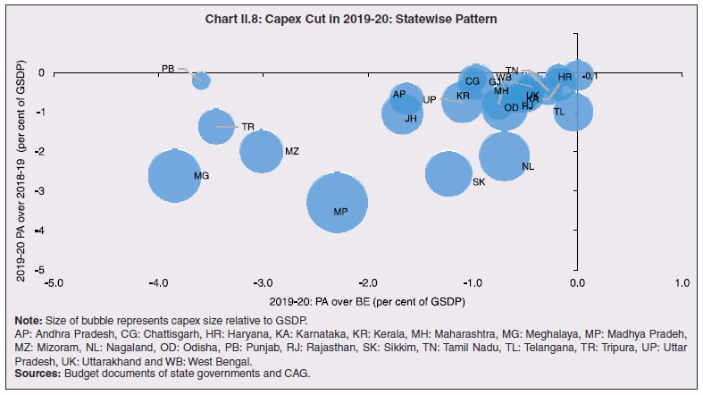
Source: Budget documents of state governments. | 2.12 Capital expenditure undertaken by states, which accounts for more than 60 per cent of general government capital expenditure is generally treated as a residual and is prone to adjustment, conditional upon revenue generation. In 2017-18 and 2018-19 as well, capital spending was reduced from budgeted levels (Table II.4). 4. 2019-20: Revised Estimates and Provisional Accounts 2.13 Drawing inference from Box II.1, the RE for 2019-20 is discussed only for expenditure composition, as the same is not available for the PA. 2.14 Despite lower revenue collection (as reflected in RE as well as in PA), states maintained revenue spending closer to 2018-19 levels, albeit lower than budgeted levels, with a re-allocation towards development expenditure (Chart II.6). As per PA, however, there is a perceptible decline in revenue spending, although break-up is not available (Table 1 of Box II.1). 2.15 Committed expenditure also rose, particularly pension payments (Chart II.7). Notably, allocation of spending towards farm loan waivers went up in 2019-20 (Table II.5). 2.16 The reduction in capital spending vis-a-vis BE observed in 2017-18 and 2018-19 recurred in 2019-20 on account of lower revenue accretion and was mainly concentrated in the rural development and irrigation sectors. 2.17 During 2019-20 as per PA, all states cut capex not only against budgeted levels, but also vis-à-vis the previous year, with all states remaining in the negative quadrant (Chart II.8). 
| Table II.5: Fiscal Impact of States’ Farm Loan Waiver Programmes | | (₹ crore) | | State | Announcement Year | Amount Announced | Budgeted Amount | | 2014-15 | 2015-16 | 2016-17 | 2017-18 | 2018-19 | 2019-20 (RE) | 2020-21 (BE) | | 1 | 2 | 3 | 4 | 5 | 6 | 7 | 8 | 9 | 10 | | Andhra Pradesh | 2014-15 | 24,000 | 4,000 | 742 | 3,512 | 3,602 | 875 | - | - | | | | | (0.8) | (0.1) | (0.5) | (0.5) | (0.1) | - | - | | Telangana | 2014-15 | 17,000 | 4,250 | 4,250 | 2,957 | 4,016 | 20 | 6,000 | 6,225 | | | | | (0.8) | (0.7) | (0.4) | (0.5) | (0.0) | (0.6) | (0.6) | | Tamil Nadu | 2016-17 | 5,280 | - | - | 1,682 | 1,870 | 884 | 807 | 735 | | | | | - | - | (0.1) | (0.1) | (0.1) | (0.0) | (0.0) | | Maharashtra | 2017-18 | 34,020 | - | - | - | 15,020 | 3,517 | - | - | | | | | - | - | - | (0.6) | (0.1) | - | - | | Maharashtra | 2019-20 | 15,000 | - | - | - | - | - | 16,931 | - | | | | | - | - | - | - | - | (0.6) | - | | Maharashtra | 2020-21 | 7,000 | - | - | - | - | - | - | 7,001 | | | | | - | - | - | - | - | - | (0.2) | | Uttar Pradesh | 2017-18 | 36,360 | - | - | - | 21,102 | 3,732 | 540 | 317 | | | | | - | - | - | (1.4) | (0.2) | (0.0) | (0.0) | | Punjab | 2017-18 | 10,000 | - | - | - | 348 | 4,238 | 2,000 | 2,000 | | | | | - | - | - | (0.1) | (0.8) | (0.3) | (0.3) | | Karnataka | 2018-19 | 44,000 | - | - | - | 3,917 | 12,640 | 5,176 | 441 | | | | | - | - | - | (0.3) | (0.8) | (0.3) | (0.0) | | Rajasthan | 2018-19 | 18,000 | - | - | - | - | 3,000 | 4,271 | 4,173 | | | | | - | - | - | - | (0.3) | (0.4) | (0.4) | | Madhya Pradesh | 2018-19 | 36,500 | - | - | - | - | - | - | - | | | | | - | - | - | - | - | - | - | | Chhattisgarh | 2018-19 | 6,100 | - | - | - | - | 3,250 | 4,984 | - | | | | | - | - | - | - | (1.1) | (1.5) | - | | Jharkhand | 2020-21 | 2,000 | - | - | - | - | - | - | 2,000 | | | | | - | - | - | - | - | - | (0.5) | | Total | | 2,31,260 | 8,250 | 4,992 | 8,151 | 49,875 | 32,156 | 40,708 | 22,893 | | Per cent of states’ total expenditure | | | 0.4 | 0.2 | 0.3 | 1.8 | 1.0 | 1.1 | 0.6 | | Per cent of GDP | | | 0.1 | 0.0 | 0.1 | 0.3 | 0.2 | 0.2 | 0.1 | RE: Revised Estimates. BE: Budget Estimates. ‘- ‘: Not available/Not applicable.
Note: Figures in parentheses indicate loan waiver as a percentage of GSDP for the corresponding year.
Source: Budget documents of state governments. |
 2.18 Although states have been conservative in adhering to FRL targets even at the cost of cutting capital spending, several factors impinging on states’ spending decisions pose challenging trade-offs (Box II.2). Box II.2: Determinants of States’ Discretionary Spending States’ total primary spending (total spending less interest payments) is considered as an indicator of discretionary spending2, driven by policy considerations rather than macroeconomic conditions. States’ discretionary spending remained at around 13 per cent of GDP in the pre-global financial crisis period (Chart 1). Since 2015, however, discretionary spending has risen in response to exogenous fiscal shocks in the form of UDAY, farm loan waivers and income support schemes (RBI, 2019a). In a panel framework for 14 non-special category3 Indian states covering the time period 1980-81 to 2012-13, capital outlay is observed to be procyclical and primary revenue expenditure is acyclical (not linked to the business cycle) (RBI, 2014). For the current analysis, discretionary spending measured by primary expenditure is modelled as follows (Arena and Revilla, 2009; Sturzenegger and Werneck (2006):  where i=1, 2…..N, indicate number of states; t =1, 2……T, indicate number of years; α represents state fixed effects which control for heterogeneity across states; primary expenditure is the governments’ discretionary spending; GSDP growth captures the state of the economy; debt or outstanding liabilities of state governments reflects sustainability of government finances; election is represented by a dummy variable taking the value 1 in the election year (to capture spending in an election year), and 0 otherwise; calamities is a dummy variable taking the value 1 if a state is affected by natural calamities such as drought, floods and cyclones, and 0 otherwise; and ε is an error term. The variables primary expenditure and debt are expressed as ratios of GSDP. The variables relating to the output gap and debt are used as two interactive dummies to examine asymmetric reactions of discretionary spending to impulse therefrom. The variable GSDP growth is interacted with positive and negative output gaps separately. The debt variable is also separated via two interactive dummies – high debt (above 25 per cent of GSDP) and low debt (less than or equal to 25 per cent of GSDP)4. A dummy for FRL implementation is also incorporated, i.e., 1 for the year states have been under this rule and 0 otherwise. Base results indicate that debt plays an important role in states’ spending decisions. Spending sensitivity to debt seems asymmetric, negative and significant at higher levels of debt (greater than 25 per cent). States’ discretionary spending is also inclined towards pro-cyclicality. Natural calamities are statistically significant and surprisingly, influence discretionary spending adversely5. The other two dummies are not statistically significant. Table 1: Two-Step System Generalized Method of Moments (GMM) Results
Dependent Variable: Primary Expenditure | | | Base Equation | Asymmetry 1 (Debt) | Asymmetry 2 (State of the Economy) | | 1 | 2 | 3 | 4 | 5 | 6 | 7 | | Primary Exp (-1) | .373** | .379** | .049 | .067 | .240 | .269 | .333 | | | (.170) | (.143) | (.321) | (.359) | (.310) | (.315) | (.231) | | GSDP Growth | .233* | .165 | .182 | .173 | .107 | | | | | (.129) | (.104) | (.111) | (.106) | (.120) | | | | Debt (-1) | -.105*** | -.073* | -.134*** | | | -.117* | -.140** | | | (.034) | (.035) | (.044) | | | (.060) | (.051) | | FRL Dum | | .764 | 1.315 | 1.177 | 1.078 | 1.519 | 1.522* | | | | (.717) | (1.001) | (.868) | (.847) | (1.428) | (.770) | | Calamities Dum | | | -6.179** | -6.734** | -6.376* | -6.195 | -4.572 | | | | | (2.883) | (2.788) | (3.189) | (5.165) | (3.899) | | Election Dum | | | -.408 | -.311 | -.441 | -.960 | -.570 | | | | | (.868) | (.780) | (.876) | (.897) | (.624) | | Debt>25% | | | | -.086* | | | | | | | | | (.042) | | | | | Debt<=25% | | | | | .167 | | | | | | | | | (.156) | | | | GSDP*Output Gap pos | | | | | | -.114 | | | | | | | | | (.139) | | | GSDP*Output Gap neg | | | | | | | .207* | | | | | | | | | (.113) | | Constant | 14.003*** | 12.964*** | 21.426** | 18.987** | 12.495** | 17.017** | 15.617** | | | (3.989) | (3.647) | (7.823) | (8.35) | (4.953) | (6.938) | (5.644) | | Observations | 396 | 396 | 396 | 396 | 396 | 396 | 396 | | Group/Instruments | 22/18 | 22/18 | 22/18 | 22/18 | 22/18 | 22/18 | 22/18 | | F-Statistics | 0.004 | 0.003 | 0.004 | 0.009 | 0.028 | 0.027 | 0.006 | | AR (2) | 0.174 | 0.133 | 0.662 | 0.550 | 0.340 | 0.804 | 0.341 | | Hansen | 0.229 | 0.274 | 0.367 | 0.443 | 0.429 | 0.212 | 0.612 | Note: ***, ** and * are statistical significance at the 1, 5 and 10 per cent levels, respectively; t statistics in parentheses are based on White heteroscedasticity-consistent standard errors; p-values reported for AR (2) and Hansen statistics.
Source: RBI staff estimates. |
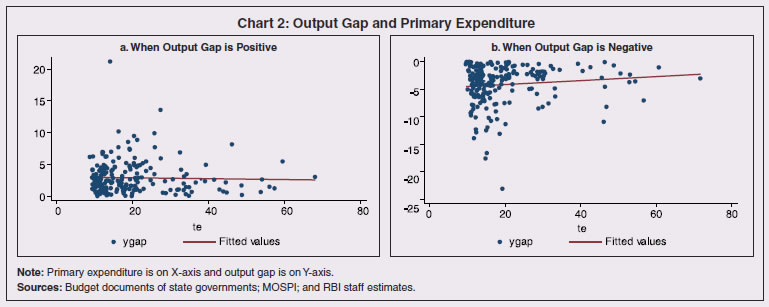 Finally, there is an asymmetric response of states’ spending to GSDP growth (Table 1; Chart 2). When actual output is above potential, states’ decisions on spending have acyclical characteristics. On the other hand, when output is below potential, states’ spending tends to get pro-cyclical, primarily by cutting spending on the capex front to accommodate for cyclical revenue shortfall. To sum up, the prominent factors influencing states’ discretionary spending decisions are debt and GSDP growth. References: Arena, Marco and Julio E. Revilla (2009). “Procyclical Fiscal Policy in Brazil - Evidence from the States”. Policy Research Working Paper series No. 5144. The World Bank. December. Reserve Bank of India. (2014). State Finances: A Study of Budgets of 2014-15. ………………………. (2019a). State Finances: A Study of Budgets of 2019-20. Sturzenegger, Fredrico and Rogerio L.F.Werneck. (2006). “Fiscal Federalism and Pro-cyclical spending: The cases of Argentina and Brazil”. Economica La Plata. Volume LII. No. 1-2. | 5. 2020-21: Budget Estimates and Actual so far 2.19 For 2020-21, states have budgeted the combined GFD at 2.8 per cent of GDP; more than half of them have budgeted for revenue surpluses (Table II.6). As explained earlier, COVID-19 is likely to undermine fiscal targets and associated receipts for 2020-21 (BE). The crisis literature focuses on the operation of the scissor effects - loss of revenues due to demand slowdown, coupled with higher expenditure associated with the pandemic (Blochliger et al., 2010; OECD, 2020b). The duration of stress on state finances will likely be contingent upon factors like tenure of lockdown and risks of renewed waves of infections, all of which make traditional backward-looking tax buoyancy forecasting models unreliable. | Table II.6: Deficit Indicators of State Governments - State-wise | | (Per cent) | | State | 2017-18 | 2018-19 | 2019-20 (RE) | 2020-21 (BE) | | RD/ GSDP | GFD/ GSDP | PD/ GSDP | RD/ GSDP | GFD/ GSDP | PD/ GSDP | RD/ GSDP | GFD/ GSDP | PD/ GSDP | RD/ GSDP | GFD/ GSDP | PD/ GSDP | | 1 | 2 | 3 | 4 | 5 | 6 | 7 | 8 | 9 | 10 | 11 | 12 | 13 | | 1 | Andhra Pradesh | 2.0 | 4.1 | 2.3 | 1.6 | 4.1 | 2.3 | 2.7 | 4.2 | 2.5 | 1.7 | 4.4 | 2.6 | | 2 | Arunachal Pradesh | -12.8 | 1.4 | -0.7 | -15.3 | 8.0 | 5.9 | -12.8 | 3.1 | 0.8 | -21.3 | 2.4 | 0.1 | | 3 | Assam | 0.5 | 3.3 | 2.1 | -2.1 | 1.5 | 0.3 | -0.2 | 6.1 | 4.7 | -2.3 | 2.4 | 0.9 | | 4 | Bihar | -3.2 | 3.1 | 1.1 | -1.3 | 2.6 | 0.7 | 3.0 | 9.5 | 7.7 | -2.8 | 2.9 | 1.1 | | 5 | Chhattisgarh | -1.2 | 2.5 | 1.4 | -0.2 | 2.7 | 1.5 | 2.9 | 6.4 | 4.9 | -0.7 | 3.2 | 1.6 | | 6 | Goa | -0.7 | 2.3 | 0.5 | -0.5 | 2.5 | 0.6 | -0.3 | 5.0 | 3.1 | -0.4 | 5.3 | 3.3 | | 7 | Gujarat | -0.4 | 1.6 | 0.2 | -0.2 | 1.8 | 0.4 | -0.1 | 1.6 | 0.3 | 0.0 | 1.8 | 0.5 | | 8 | Haryana | 1.6 | 2.9 | 1.1 | 1.5 | 3.0 | 1.1 | 1.8 | 2.8 | 0.9 | 1.6 | 2.7 | 0.8 | | 9 | Himachal Pradesh | -0.2 | 2.8 | 0.1 | -1.0 | 2.3 | -0.3 | 2.4 | 6.4 | 3.7 | 0.4 | 4.0 | 1.3 | | 10 | Jharkhand | -0.7 | 4.4 | 2.7 | -2.0 | 2.1 | 0.5 | -2.0 | 2.4 | 0.8 | -0.5 | 2.2 | 0.7 | | 11 | Karnataka | -0.3 | 2.3 | 1.3 | 0.0 | 2.5 | 1.5 | 0.0 | 2.3 | 1.2 | 0.0 | 2.6 | 1.3 | | 12 | Kerala | 2.4 | 3.8 | 1.7 | 2.2 | 3.4 | 1.3 | 2.0 | 3.0 | 0.9 | 1.6 | 3.0 | 1.0 | | 13 | Madhya Pradesh | -0.6 | 3.1 | 1.6 | -1.1 | 2.7 | 1.1 | 0.3 | 3.6 | 2.1 | 1.8 | 5.0 | 3.3 | | 14 | Maharashtra | -0.1 | 1.0 | -0.4 | -0.5 | 0.9 | -0.4 | 1.1 | 2.7 | 1.5 | 0.3 | 1.7 | 0.6 | | 15 | Manipur | -4.2 | 1.3 | -0.9 | -2.9 | 3.3 | 1.2 | -0.9 | 8.5 | 6.8 | -5.6 | 3.8 | 2.2 | | 16 | Meghalaya | -2.9 | 0.5 | -1.5 | 1.6 | 6.1 | 4.1 | -2.0 | 3.6 | 1.6 | -2.3 | 3.8 | 1.7 | | 17 | Mizoram | -9.1 | 1.7 | -0.1 | -7.9 | 1.8 | -0.1 | 2.8 | 10.4 | 8.7 | -3.3 | 2.3 | 0.7 | | 18 | Nagaland | -3.4 | 1.8 | -0.9 | -1.9 | 4.0 | 1.1 | 1.9 | 8.0 | 5.1 | -3.0 | 4.0 | 1.1 | | 19 | Odisha | -3.0 | 2.1 | 1.0 | -2.9 | 2.1 | 0.9 | -1.2 | 3.4 | 2.2 | -1.6 | 3.0 | 1.8 | | 20 | Punjab | 2.0 | 2.7 | -0.6 | 2.5 | 3.1 | 0.0 | 2.2 | 3.0 | -0.1 | 1.2 | 2.9 | 0.0 | | 21 | Rajasthan | 2.2 | 3.0 | 0.7 | 3.1 | 3.7 | 1.4 | 2.7 | 3.2 | 0.8 | 1.1 | 3.0 | 0.7 | | 22 | Sikkim | -4.1 | 1.8 | 0.4 | -2.4 | 2.2 | 0.7 | -0.2 | 3.7 | 2.1 | -1.7 | 2.8 | 1.3 | | 23 | Tamil Nadu | 1.5 | 2.7 | 0.9 | 1.4 | 2.9 | 1.1 | 1.4 | 3.0 | 1.3 | 1.0 | 2.8 | 1.1 | | 24 | Telangana | -0.5 | 3.5 | 2.1 | -0.5 | 3.1 | 1.7 | 0.0 | 2.3 | 0.8 | -0.4 | 3.0 | 1.7 | | 25 | Tripura | 0.7 | 4.7 | 2.7 | -0.3 | 2.7 | 0.6 | 3.8 | 6.5 | 4.4 | 0.4 | 3.5 | 1.4 | | 26 | Uttar Pradesh | -0.9 | 1.9 | -0.1 | -1.7 | 2.1 | 0.2 | -1.5 | 2.8 | 0.9 | -1.4 | 2.7 | 0.8 | | 27 | Uttarakhand | 0.9 | 3.6 | 1.8 | 0.4 | 3.0 | 1.2 | 0.0 | 2.5 | 0.6 | 0.0 | 2.6 | 0.6 | | 28 | West Bengal | 1.0 | 3.0 | 0.1 | 1.0 | 3.1 | 0.4 | 0.5 | 2.7 | 0.2 | 0.0 | 2.2 | -0.1 | | 29 | Jammu and Kashmir | -5.5 | 2.0 | -1.4 | 3.1 | 8.5 | 5.1 | -4.4 | 7.1 | 5.0 | -12.8 | 5.3 | 1.7 | | 30 | NCT Delhi | -0.7 | 0.0 | -0.4 | -0.8 | -0.3 | -0.7 | -1.1 | -0.1 | -0.4 | -0.8 | 0.5 | 0.2 | | 31 | Puducherry | -0.6 | 0.6 | -1.5 | 0.0 | 0.8 | -1.1 | -0.3 | 0.8 | -1.0 | 1.0 | 1.8 | 0.2 | | All States and UTs | 0.1 | 2.4 | 0.7 | 0.1 | 2.4 | 0.8 | 0.7 | 3.2 | 1.5 | 0.0 | 2.8 | 1.1 | RE: Revised Estimates. BE: Budget Estimates. RD: Revenue Deficit. GFD: Gross Fiscal Deficit. PD: Primary Deficit.
GSDP: Gross State Domestic Product.
Note: Negative (-) sign in deficit indicators indicates surplus.
Source: Budget documents of state governments. | Crisis hampers compliance culture as countries defer filing/payment dates to enhance cash flows in the hands of taxpayers or to encourage social distancing (IMF, 2020 a and d6). Under such circumstances, uncertainty around central forecasts has to be captured either through fan charts (as in case of UK) or by building up forward-looking scenarios. Receipts 2.20 In anticipation of a recovery of economic activity in 2020-21, states budgeted for higher tax revenue collection, with broad-based increases in all tax components. Developments in the first half of the year have completely belied these expectations. It is increasingly certain that the slump in economic activity due to COVID-19 led lockdown will adversely impact states’ revenue collections. The implied tax buoyancy for 2020-21 (based on 2019-20 PA) is higher than budgeted on the basis of 2019-20 RE and much higher than previous year’s average (Table II.7). 2.21 The major head under states’ own tax revenue, viz., taxes on commodities and services would be impacted the most. SGST plummeted by 47.2 per cent during Q1:2020-21 - sharper than the overall GST decline - with variations contingent upon state-specific spatial features. During Q2, however, the decline moderated to 6.4 per cent. 2.22 Stamp duties, which are a major source of revenue under states’ direct taxes, are also likely to witness a shortfall, consequent upon contraction in construction activity, reverse migration of labourers and social distancing norms. Furthermore, revenue specific measures, viz., extension of deadlines for payment of taxes to provide relief to businesses and citizens may further exacerbate the already worsening revenue situation of states. Monthly analysis of the data for April - June 2020 gives a glimpse of the deterioration, with revenue collections having seen the steepest year on year (y-o-y) fall across the majority of states, though with unlocking in phases, July 2020 data available for few states shows marginal improvement (Chart II.9). 2.23 Nonetheless, in order to garner some additional revenues during these unprecedented times, 22 states/UTs have hiked their duties on petrol and diesel, while 25 states/UTs have hiked duties on alcohol. The consequent rise in petrol /diesel prices is in the range of 60 paisa to ₹8, while for alcohol, it is in the range of 10-120 per cent, on an average basis (Chart II.10a and b). This is expected to provide a revenue gain in the range of 0.03 to 0.35 per cent of GSDP. Petroleum and alcohol, on an average, account for 25-35 per cent of the own tax revenue of states (RBI, 2019a) (Chart II.10c). | Table II.7: Tax Buoyancy of States’ Own Tax Revenue | | | 2013-14 | 2014-15 | 2015-16 | 2016-17 | 2017-18 | 2018-19 | 2019-20 | 2020-21 BE | | 1 | 2 | 3 | 4 | 5 | 6 | 7 | 8 | 9 | | Based on 2019-20 RE | | | | | | | 1.49 | 1.18 | | As per Actual/ PA | 0.68 | 0.83 | 0.85 | 0.65 | 1.75 | 0.69 | 0.92 | 1.61 | | Sources: Budget documents of state governments; CAG; and RBI staff estimates. |
2.24 Another major source of revenue for states is tax transfers from the centre from the divisible pool. Of the total revenue receipts of states, central tax transfers comprise 25 to 29 per cent, while own tax revenues have a share of 45 to 50 per cent. Given that a large shortfall in the divisible pool is highly likely in 2020-21, central tax transfers to states could fall by a significant margin. Automatic stabilisers inherent in states’ own tax revenue and central tax transfers, albeit low, could be important in low growth phases, when both components are taken together (Box II.3). 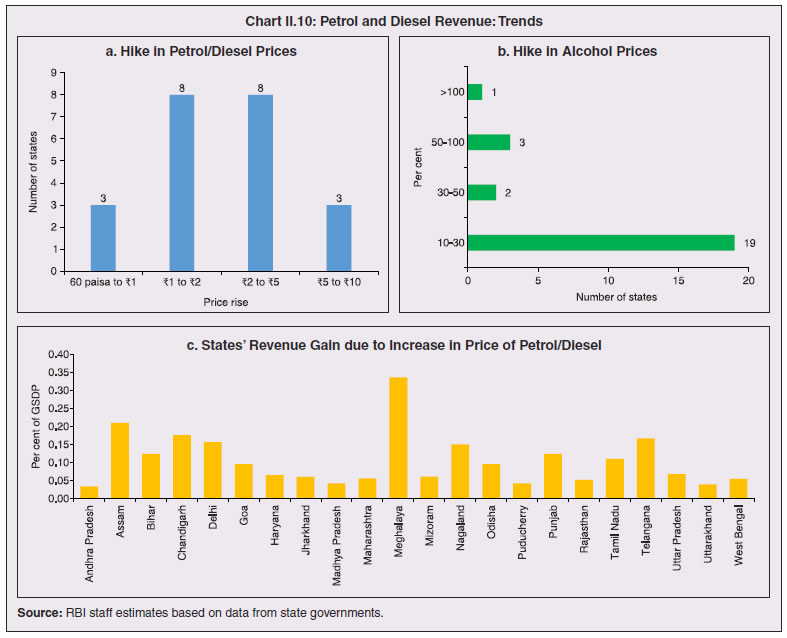
Box II.3: Automatic Stabilisers in States’ Own Tax Revenue and Transfers Automatic stabilisers for own tax revenue and central tax transfers are calculated on the basis of tax elasticities and output gap estimates (following Fedelino et al., 2009). The elasticity of central tax transfers with respect to GDP captures the dynamics of tax performance of the Union Government of India and is generally higher than the states’ own tax elasticity in view of the progressive nature of the taxes in the centre’s kitty7. Regressing states’ own tax revenue growth on GDP growth in a co-integrated framework with suitable dummies for policy changes yields a long run elasticity of about 1.0. In view of statistical evidence of regime shifts revealed by the Wald test, short run tax elasticities are estimated by applying Markov switching regressions (Hamilton, 1989), assuming variance to be common for both the regimes. The implementation of VAT and GST are captured through dummies. The results indicate two distinct elasticities for the high and low growth regimes, with higher growth associated with lower tax elasticity and vice versa (Chart 1). With the pandemic expected to produce negative nominal GDP growth, not part of estimation series, tax elasticity could be even higher8. The overall automatic stabiliser for states, combining both own tax revenue and the central tax revenues component, albeit low in the range of 10-30 bps of GDP, is observed to be significant during low growth years (Chart 2). References Fedelino, A., Anna I., and Mark H. 2009. Cyclically Adjusted Balances and Automatic Stabilizers: Some Computation and Interpretation Issues. IMF Technical Notes and Manuals. Hamilton, J. D. (1989). “A new approach to the economic analysis of nonstationary time series and the business cycle” Econometrica. 57: 357-384. | 2.25 Revenue receipts are likely to be cushioned by revenue deficit grants, which compensate for deficits that prevail even after devolution, and the GST compensation cess, which states are stipulated to receive if their revenues fall below a threshold in any particular year (GST Compensation Cess Act, 2017). The share of grants is particularly high for special category states, mainly due to higher revenue deficit grants (Chart II.11). It may be noted that with an increase in revenue deficit grants by ₹44,340 crores in the additional supplementary demand for grants announced by the centre in September 2020 on top of the budgeted ₹30,000 crore on February 1, 2020, it has released the full quantity of revenue deficit grants as recommended by the Fifteenth Finance Commission (FC-XV). Accordingly, the revenue deficit grants in 2020-21 are more than double the average of the previous few years. 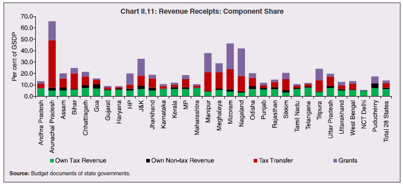 2.26 As regards GST compensation cess, states have received the full GST compensation in the first three years of GST implementation. Unlike 2017-18 and 2018-19, for 2019-20, amount transferred to states was higher than collections during the year (Table II.8). Nevertheless, the high uncertainty associated with the quantum of GST cess collections by the centre, coupled with ambiguity around the timing and amount of compensation transfer9, has raised concerns. In 2020-21, while ₹ 65,000 cess collections are expected, the Centre has decided to borrow an additional ₹1.1 lakh crore in tranches in H2:2020-21 to provide compensation to states for shortfall in their revenue in 2020-21 arising on account of GST implementation. The amount so borrowed will be passed on to states as a loan, in lieu of GST compensation cess release, and will reflect as capital receipts of state governments, going into the financing of respective fiscal deficits10. | Table II.8: GST Compensation Cess | | (₹ crore) | | | 2017-18 | 2018-19 | 2019-20 | | 1 | 2 | 3 | 4 | | Compensation Cess Collected | 62,612 | 95,081 | 95,444 | | Compensation Cess Transferred to States | 48,785 | 81,141 | 1,65,302 | | Sources: Press Information Bureau; Lok Sabha Unstarred Question and Dept. of Revenue, Ministry of Finance. | Expenditure 2.27 States have budgeted for reduction in revenue expenses in 2020-21 vis-à-vis 2019-20 RE, and a higher capital expenditure in 2020-21 vis-à-vis 2019-20 RE, mostly in social services under capital outlay. While higher spending is budgeted in education, water supply and sanitation, rural and urban development, spending on energy and transport is expected to be curtailed (Table II.9). | Table II.9: Variation in Major Components | | (₹ lakh crore) | | Item | 2016-17 | 2017-18 | 2018-19 | 2019-20 (RE) | 2020-21 (BE) | Percent Variation | | 2019-20 RE over 2018-19 | 2020-21 BE over 2019-20 | | 1 | 2 | 3 | 4 | 5 | 6 | 7 | 8 | | I. Revenue Receipts (i+ii) | 20.86 | 23.21 | 26.20 | 29.40 | 33.27 | 12.2 | 13.2 | | (i) Tax Revenue (a+b) | 15.54 | 17.36 | 19.62 | 20.43 | 23.16 | 4.2 | 13.3 | | (a) Own Tax Revenue | 9.46 | 11.30 | 12.15 | 13.40 | 14.98 | 10.3 | 11.8 | | of which: Sales Tax | 6.10 | 4.02 | 2.89 | 3.11 | 3.42 | 7.7 | 10.1 | | (b) Share in Central Taxes | 6.08 | 6.05 | 7.47 | 7.03 | 8.17 | -5.8 | 16.2 | | (ii) Non-Tax Revenue (a+b) | 5.32 | 5.86 | 6.59 | 8.96 | 10.12 | 36.1 | 12.9 | | (a) States' Own Non-Tax Revenue | 1.71 | 1.80 | 2.19 | 2.39 | 2.68 | 9.3 | 12.1 | | (b) Grants from Centre | 3.61 | 4.06 | 4.40 | 6.57 | 7.43 | 49.4 | 13.1 | | II. Revenue Expenditure | 21.22 | 23.40 | 26.38 | 30.76 | 33.27 | 16.6 | 8.2 | | of which: | | | | | | | | | (i) Development Expenditure | 13.66 | 14.66 | 16.36 | 19.46 | 20.68 | 19.0 | 6.2 | | of which: Education, Sports, Art and Culture | 3.95 | 4.25 | 4.68 | 5.40 | 5.89 | 15.4 | 9.0 | | Transport and Communication | 0.48 | 0.51 | 0.51 | 0.57 | 0.64 | 11.8 | 12.3 | | Power | 1.33 | 1.16 | 1.29 | 1.55 | 1.33 | 20.1 | -14.5 | | Relief on account of Natural Calamities | 0.28 | 0.16 | 0.30 | 0.49 | 0.35 | 63.3 | -28.6 | | Rural Development | 1.26 | 1.32 | 1.38 | 1.73 | 1.89 | 25.8 | 9.4 | | (ii) Non-Development Expenditure | 6.99 | 8.06 | 9.22 | 10.36 | 11.64 | 12.3 | 12.4 | | of which: Administrative Services | 1.47 | 1.62 | 1.84 | 2.20 | 2.56 | 19.5 | 16.4 | | Pension | 2.27 | 2.75 | 3.15 | 3.55 | 3.86 | 12.7 | 8.6 | | Interest Payments | 2.55 | 2.93 | 3.19 | 3.49 | 3.89 | 9.3 | 11.4 | | III. Net Capital Receipts # | 5.61 | 4.55 | 5.06 | 6.50 | 6.26 | 28.6 | -3.9 | | of which: Non-Debt Capital Receipts | 0.16 | 0.40 | 0.42 | 0.62 | 0.20 | 47.6 | -67.7 | | IV. Capital Expenditure $ | 5.17 | 4.31 | 4.87 | 5.78 | 6.46 | 18.6 | 11.8 | | of which: Capital Outlay | 3.96 | 3.94 | 4.40 | 5.31 | 5.98 | 20.6 | 12.7 | | of which: Capital Outlay on Irrigation and Flood Control | 0.83 | 0.83 | 0.93 | 0.92 | 1.05 | -1.1 | 14.1 | | Capital Outlay on Energy | 0.53 | 0.46 | 0.43 | 0.54 | 0.31 | 25.5 | -42.0 | | Capital Outlay on Transport | 0.96 | 0.93 | 1.14 | 1.33 | 1.33 | 16.7 | 0.0 | | Memo Item: | | Revenue Deficit | 0.36 | 0.19 | 0.18 | 1.37 | 0.00 | 661.1 | -100.0 | | Gross Fiscal Deficit | 5.36 | 4.10 | 4.63 | 6.52 | 6.26 | 40.8 | -4.0 | | Primary Deficit | 2.81 | 1.17 | 1.44 | 3.04 | 2.38 | 111.1 | -21.7 | RE: Revised Estimates. BE: Budget Estimates.
# : It includes following items on net basis - Internal Debt, Loans and Advances from the Centre, Inter-State Settlement, Contingency Fund, Small Savings, Provident Funds etc., Reserve Funds, Deposits and Advances, Suspense and Miscellaneous and Appropriation to Contingency Fund and Remittances.
$ : Capital Expenditure includes Capital Outlay and Loans and Advances by State Governments.
Notes: 1. Negative (-) sign in deficit indicators indicates surplus.
2. Also see Notes to Appendices.
Source: Budget documents of state governments. |
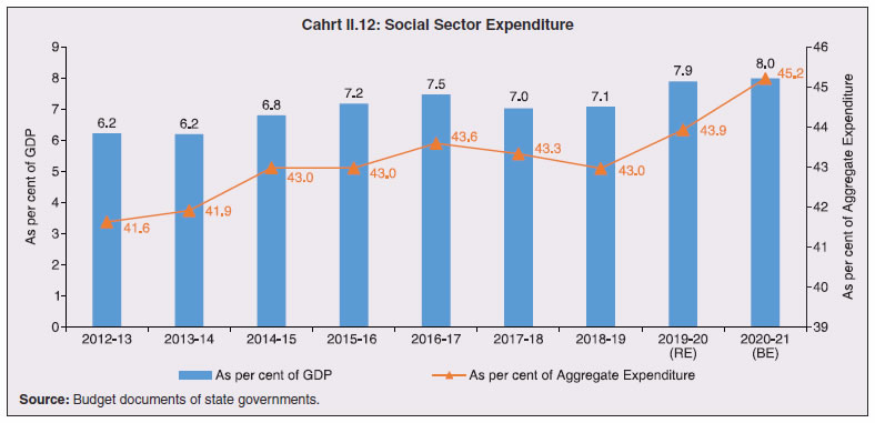 2.28 Social sector expenditure has been increasing since 2018-19 and is budgeted to reach 8.0 per cent of GDP in 2020-21 (Chart II.12). 2.29 In social sector spending, the share of urban development and welfare of SCs, STs and OBCs has seen a clear rise, while all other expenditures are either declining or are stagnant (Table II.10). 2.30 The pandemic has necessitated fiscal policy actions to boost aggregate demand. Table II.10: Composition of Expenditure on Social Services
(Revenue and Capital Accounts) | | (Per cent of expenditure on social services) | | Item | 2015-16 | 2016-17 | 2017-18 | 2018-19 | 2019-20 (RE) | 2020-21 (BE) | | 1 | 2 | 3 | 4 | 5 | 6 | 7 | | Expenditure on Social Services (a to l) | 100.0 | 100.0 | 100.0 | 100.0 | 100.0 | 100.0 | | (a) Education, Sports, Art and Culture | 44.0 | 43.0 | 42.9 | 41.8 | 40.8 | 40.3 | | (b) Medical and Public Health | 11.6 | 11.8 | 12.3 | 12.3 | 12.1 | 12.1 | | (c) Family Welfare | 2.0 | 1.9 | 2.0 | 2.1 | 2.0 | 2.0 | | (d) Water Supply and Sanitation | 6.1 | 6.5 | 7.0 | 6.6 | 6.5 | 6.5 | | (e) Housing | 2.9 | 3.2 | 3.8 | 3.5 | 3.2 | 4.0 | | (f) Urban Development | 6.5 | 8.0 | 7.6 | 7.6 | 8.4 | 9.7 | | (g) Welfare of SCs, STs and OBCs | 7.0 | 6.9 | 7.4 | 6.9 | 8.0 | 8.4 | | (h) Labour and Labour Welfare | 0.9 | 0.8 | 0.9 | 1.0 | 1.0 | 1.0 | | (i) Social Security and Welfare | 11.4 | 10.9 | 10.4 | 11.9 | 10.9 | 9.9 | | (j) Nutrition | 2.6 | 2.4 | 2.3 | 2.1 | 2.2 | 2.2 | | (k) Expenditure on Natural Calamities | 3.9 | 2.9 | 1.6 | 2.6 | 3.6 | 2.3 | | (l) Others | 1.1 | 1.6 | 1.8 | 1.6 | 1.3 | 1.5 | RE: Revised Estimates. BE: Budget Estimates.
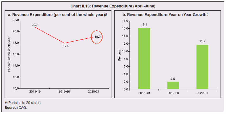
Source : Budget documents of state governments. | Alongside the centre, state governments have been proactive in undertaking policy measures to contain the impact of the pandemic (Table II.11). The financial supports are in the form of insurance cover for doctors and nurses; purchase of medical equipment and tools; hospital arrangements with a sufficient number of beds for COVID-19 patients; providing food free of cost; cash for those who are not availing of any government schemes; cash for registered construction workers; remitting a fixed sum for those trapped abroad in other states; and advance salary and pension payments. Quantifying the various kinds of policy measures, the fiscal stimulus works to about 0.3 per cent of GDP11. 2.31 Monthly data on revenue expenditure during April-June 2020 show no significant increase when compared with corresponding months of previous few years (Chart II.13). Although states generally receive and spend about one fifth of their budgeted allocations during Q1 each year, they have maintained their spending at previous years’ levels in 2020-21, despite receiving only one-eighth of their budgeted revenues. | Table II.11: State-wise Policy Measures to Contain the Adverse Impacts of Pandemic | | Measure | State Specific Effort | | Health Expenditure | • Fund for scaling up health infrastructure (screening facilties, lab equipments, ventilators) by Andhra Pradesh, Jharkhand, UP, Uttarakhand, J&K, MP (telemedicine facility also) and Chattisgarh
• Assam announced to bear the treatment cost of COVID-19 patients
• Odisha earmarked a separate amount to augment its Public Health Response Fund
• Rajasthan, Tamil Nadu, West Bengal and Sikkim have provided additional funding to their health departments
• UP created a Corona Care Fund for setting up testing facilities and provision made for providing medical facilities.
• West Bengal enhanced insurance coverage for medical staff. Tamil Nadu has set up a corpus fund under a new health insurance scheme for the treatment of government employees and pensioners infected by COVID-19.
• Tripura flagged off emergency life support ambulances. Tamil Nadu has also purchased additional ambulances.
• Gujarat distributed free N-95 masks to doctors. Tamil Nadu introduced a scheme for distributing free face masks to all family card holders in districts other than Chennai through fair price shops.
• Karnataka has announced various incentives for ASHA workers and other frontline workers of COVID-19. | | Social Assistance to Vulnerable Sections | Assam, Bihar, Kerala, Andhra Pradesh, Odisha, Punjab, Sikkim, Tamil Nadu, Telangana, UP, Himachal Pradesh, West Bengal, Rajasthan, Jammu and Kashmir, Gujarat, Karnataka and Delhi | | Free Ration | Bihar, Jharkhand, Kerala, Odisha, Punjab, Sikkim, Tamil Nadu, Telangana, UP, Manipur, Rajasthan, Jammu and Kashmir, Delhi, West Bengal, Gujarat, Andhra Pradesh, MP, Karnataka and Chhattisgarh | | Assistance to Construction Workers, Migrant Labourers and Daily Wage Workers | Bihar, Punjab, Odisha, Sikkim, Tamil Nadu, Telangana, Uttarakhand, UP, West Bengal, Himachal Pradesh, Mizoram, Delhi, Andhra Pradesh, Karnataka and Jammu and Kashmir | Note: The list may not be exhaustive as it is based on information received from states.
Source: State governments. |
 2.32 This can be also attributed to re-prioritization of expenditure by curtailment of some revenue expenditure allocations by various state governments viz., DA freeze; deferment of part or full salaries and wages and deduction from salary (Table II.12). On the whole, states’ fiscal response to COVID-19 should reflect in a larger increase in revenue expenditure in 2020-21 than budgeted. These spendings coupled with revenue receipts shortfall are likely to convert revenue surpluses as budgeted in 2020-21 into large deficits. | Table II.12: Expenditure Rationalisation by States During COVID-19 | | No. | Type of Revenue Expenditure | State | | 1 | 2 | 3 | | 1. | Deferment of part or full of salary, wages and bills | Andhra Pradesh, Assam, Mizoram, Odisha, and Telangana | | 2. | Deduction of salary | Maharashtra | | 3. | Freezing of DA | Karnataka | | 4. | Suspension of encashment facility of earned leave | Karnataka, Kerala and Tamil Nadu | | 5. | Rationalisation of travel and vehicle expenses, establishment and other expenses | Assam and Odisha | Note: The list may not be exhaustive as it is based on information received from states.
Source: State governments. | 2.33 Globally, India has the highest de-centralisation of capital expenditure12 (Chart II.14a). 2.34 Capital spending in India is not completely executed, however, and often falls short of the budgeted targets, as explained earlier. Moreover, inefficiency leads to a substantial waste of funds spent on public infrastructure across many Emerging market economies (IMF, 2020a). States have a tendency to cut back their capital expenditure by almost 0.5 per cent of GDP, on an average (Chart II.14b), to meet FRL- prescribed fiscal deficit targets. A similar tendency relative to BE can be expected in 2020-21, particularly since states have not been able to start much capex in H1 because of lockdown (in Q1) and monsoons (in Q2). As in revenue expenditure, one may see major re-adjustments and re-prioritisation as well. While the obvious focus in H1:2020-21 seems to be on capex in health and education sectors in response to the pandemic, other critical sectors like roads and construction may draw attention in H2. To drive capex, centre also recently announced a special interest free 50-year loan to states for capital expenditure of ₹12,000 crore to be spent till March 2021, albeit it represents a small fraction of budgeted capex of ₹ 6.5 lakh crores.  6. Market Borrowings13 and Projected GFD 2.35 On average, market borrowings financed slightly more than half of the consolidated fiscal deficit of states till 2016-17. Since 2017-18, however, the share of market borrowings has increased rapidly and is budgeted to reach close to 90 per cent in 2020-21 BE (Table II.13). As per 2018-19 actual, states with GFD equal to or less than 3 per cent of GSDP financed it mostly through market borrowings. States with GFD-GDP ratios of more than 3 per cent have relied on other sources, viz., withdrawal from public accounts like provident funds, deposit and advances, and cash withdrawals, being constrained by the provisions of Article 293 of the constitution14. 2.36 In a longer-term perspective, borrowing by states/UTs - gross and net - are fast catching up with those of the centre, with the drying up of all other sources of financing. The share of states’ market borrowing in general government borrowings has more than doubled in the last five years, also necessitated by rising redemptions (Chart II.15). | Table II.13: Financing Pattern of Gross Fiscal Deficit | | Item | 2016-17 | 2017-18 | 2018-19 | 2019-20 (RE) | 2020-21 (BE) | 2018-19# (Per cent of GSDP/GDP) | | GFD<=3.0 per cent | GFD>3.0 per cent | All States/ UTs | | 1 | 2 | 3 | 4 | 5 | 6 | 7 | 8 | 9 | | Financing (1 to 8) | 100.0 | 100.0 | 100.0 | 100.0 | 100.0 | 2.1 | 3.6 | 2.4 | | 1. Market Borrowings | 65.7 | 84.0 | 80.6 | 74.9 | 89.5 | 1.8 | 2.7 | 2.0 | | 2. Loans from centre | 1.0 | 1.1 | 1.9 | 1.7 | 2.8 | 0.0 | 0.1 | 0.0 | | 3. Special Securities issued to NSSF/Small Savings | -6.0 | -7.9 | -7.3 | -4.9 | -5.2 | -0.2 | -0.2 | -0.2 | | 4. Loans from LIC, NABARD, NCDC, SBI and Other Banks | 8.1 | 3.1 | 3.9 | 2.9 | 4.0 | 0.1 | 0.0 | 0.1 | | 5. Provident Fund | 7.4 | 8.2 | 10.3 | 5.2 | 5.5 | 0.2 | 0.5 | 0.3 | | 6. Reserve Funds | 3.9 | 0.9 | 3.8 | 4.5 | 2.4 | 0.1 | 0.1 | 0.1 | | 7. Deposits and Advances | 7.9 | 15.6 | 11.1 | 1.8 | 3.0 | 0.2 | 0.4 | 0.3 | | 8. Others | 11.9 | -5.1 | -4.3 | 13.9 | -2.0 | -0.1 | 0.0 | -0.1 | RE: Revised estimates. BE: Budget estimates.
NSSF: National Small Savings Fund; LIC: Life Insurance Corporation of India; NCDC: National Co-Operative Development Corporation; SBI: State Bank of India; NABARD: National Bank for Agriculture and Rural Development
#: Excludes Delhi and Puducherry.
Notes: 1. See Notes to Appendix Table 9.
2. ‘Others’ includes Compensation and Other Bonds, Loans from Other Institutions, Appropriation to Contingency Fund, Inter-State Settlement, Contingency Fund, Suspense and Miscellaneous, Remittance and Overall Surplus/Deficit.
Source: Budget documents of state governments. | 2.37 While net borrowings of the states/ UTs increased by about 40 per cent during 2019-20, gross market borrowings at ₹6.3 lakh crore increased by 32.7 per cent, one of the highest in the recent past (Table II.14). While states like Odisha and Haryana have been pragmatic in trying to meet their higher fiscal deficits by using their own rainy funds without recourse to higher permissible market borrowings, there are states like Gujarat and Punjab which have over-borrowed despite consolidation, with Uttar Pradesh being an extreme case - it has borrowed above 20 per cent of the budgeted amount, despite registering a fiscal surplus as against a budgeted deficit in 2019-20 (Chart II.16). 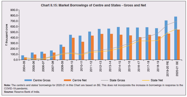
| Table II.14: Market Borrowings of State Governments | | (₹ crore) | | Item | 2017-18 | 2018-19 | 2019-20 | 2020-21* | | 1 | 2 | 3 | 4 | 5 | | Maturities during the year | 78,819 | 1,29,680 | 1,47,067 | 54,607 | | Gross sanction under Article 293(3) | 4,82,475 | 5,5,0071 | 7,12,744 | 5,77,255 | | Gross amount raised during the year | 4,19,100 | 4,78,323 | 6,34,521 | 3,53,596 | | Net amount raised during the year | 3,40,281 | 3,48,643 | 4,87,454 | 2,98,989 | | Amount raised during the year to total Sanctions (per cent) | 87 | 87 | 89 | 61 | | Weighted Average Yield of SDLs | 7.67 | 8.32 | 7.24 | 6.43 | | Weighted Average Spread over corresponding G-Sec (bps) | 59 | 65 | 55 | 53 | | Average Inter- State Spread (bps) | 6 | 6 | 6 | 9 | *: As on September 30, 2020.
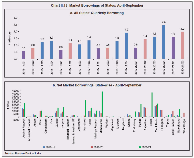
Source: Reserve Bank of India. | 2.38 For 2020-21, states had budgeted a gross borrowing of ₹7 lakh crore. Under the Aatma Nirbhar Package in May 2020, states are allowed to increase their borrowing limits from 3 per cent to 5 per cent for 2020- 21. This is expected to provide extra resources of ₹4.28 lakh crore. 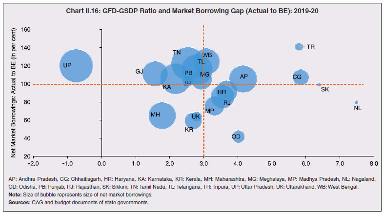 2.39 While the increase from 3 to 3.5 per cent of GDP is unconditional, which states can access after suitable revision of their FRLs (many states have promulgated ordinance to this effect)15, the balance increase in market borrowing was initially made conditional. As per the specific scheme notified by the Department of Expenditure, an additional 1 per cent of GDP will be provided in four tranches of 0.25 per cent, with each tranche linked to clearly specified, measurable and feasible reform actions in four areas: universalisation of ‘One Nation One Ration card’; ease of doing business; power distribution; and urban local body revenue reforms. While some states have already met two of the reform measures (one-nation-one-ration card and the ease of doing business), some others may pursue them during the second half. An additional 0.5 per cent was to be allowed if milestones are achieved in at least three out of four reform areas (GoI, 2020a). Subsequent to the October GSTC Council meeting, states which benefit from the special window could get this additional 0.5 per cent borrowing unconditional. This is, however, expected to have a limited impact on the fiscal deficit of state governments that are likely to borrow a considerably lesser amount from the additional borrowing facility of 2 per cent of GSDP under the Aatma Nirbhar Package. On the whole, given states past track record of not being able to access market borrowings despite higher limits, and considering the meticulous process that states need to adhere to in order to get the clearance certificate from respective Ministries/ Departments with regard to achievement of the specified reform measures for the conditional part of the borrowing within the current fiscal year, they may be able to utilise only half of the additional borrowing given to them - conditional and unconditional on an average. With borrowings financing about 90 per cent of states’ fiscal deficit, on an average, borrowing limits under Article 293 (3) act as soft constraint. Thus, from the financing side, states’ combined GFD-GDP ratio is likely to remain around 4 per cent with a bias tilted to the upside, higher than the budgeted 2.8 per cent of GDP (Chart II.17), albeit with state-wise variations. 2.40 Accordingly, in H1:2020-21, more than 60 per cent increase in borrowings on a year on year basis has already occurred, with about 7-8 states accounting for the bulk of the increase (Chart II.18 a and b). This additional borrowing, coupled with withdrawal of cash balances, are likely to be used for financing the slippage from revenue shortfall and rise in revenue expenditure. 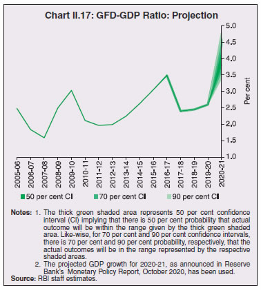
 2.41 The maturity profile of states’ debt indicates that state development loans (SDLs) redemptions are likely to more than double from 2026 onwards (Chart II.19). The weighted average (cut-off) yield (WAY) of SDLs had been rising since 2016-17 till 2018-19, although it moderated in 2019-20 to 7.24 per cent, about 108 bps lower than in 2018-19 (Chart II.19). After significant moderation in Q1:2020-21, SDL yields and spreads have been picking up in Q2. The average inter-state spread on SDLs of 10-year maturity (fresh issuance) was higher at 9 bps in H1:2020-21 (4 bps in H1:2019-20). The Reserve Bank in its Monetary Policy Statement, October 2020 has allowed open market operations (OMO) in SDLs, which may improve secondary market liquidity and lower their spreads over corresponding G-secs. The first ever such OMO of ₹10,000 crore, conducted on October 22, 2020, will purchase SDLs of Andhra Pradesh, Arunachal Pradesh, Assam, Bihar, Chhattisgarh, Goa, Gujarat, Haryana, Himachal Pradesh, Jammu and Kashmir, Jharkhand, Karnataka, Kerala, Madhya Pradesh and Maharashtra through a multi-security auction using multiple price method with no security-wise notified amount. 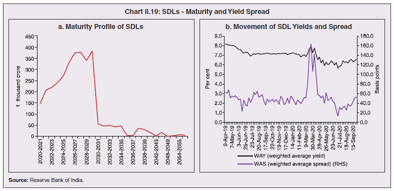 2.42 Re-issuances to enhance liquidity saw a fillip in 2019-20, with their share in overall issuances rising from 10 per cent in 2017-18 to close to 20 per cent in 2019-2016. During the year, 17 states and the UT of Puducherry issued securities of non-standard maturities, ranging between 2 and 40 years, moving away from the usual practice of issuance of 10 year paper, to elongate maturities and contain roll-over risks. At end-March 2020, 66.8 per cent of the outstanding SDLs was in the residual maturity bucket of five years and above (Table II.15). Cash Management of State Governments 2.43 States have been accumulating sizeable cash surpluses in recent years in the form of Intermediate Treasury Bills (ITBs) and Auction Treasury Bills (ATBs), involving a negative carry of interest rates and warranting improvement in cash management practices going forward (Table II.16). There is, however, evidence of utilisation of cash balances on the part of many states in H1:2020-21, notably for ITBs. Financial Accommodation by States 2.44 The ways and means advances (WMA) limits of states was reviewed by an Advisory Committee in 2016 and it recommended the limit of ₹32,225 crore for all states/UTs together. Currently, a new committee, viz., the Advisory Committee to Review the Ways and Means limits for State Governments and Union Territories (UTs) (Chairman: Shri Sudhir Shrivastava) is reviewing the WMA limits. With the onset of the COVID-19 pandemic and the strained finances of states, the Reserve Bank decided on April 1, 2020 to increase states’ WMA limit by 30 per cent from the existing limit for all states/UTs and this was increased further by 60 per cent over and above the level as on March 31, 2020, extended for a further period of 6 months till March 31, 2021. Furthermore, the number of days for overdraft (OD) has been increased, effective April 7, 2020, till September 30, 2020 and further extended till March 31, 2021. 16 states availed the Special Drawing Facility (SDF) in 2019-20, while 13 states resorted to WMA and ten states availed OD. During 2020-21 so far, utilisation of WMA has shown significant rise. 14 states and one UT have resorted to WMA during H1:2020-21. Enhanced WMA limit is availed by eight states and one UT during the same period. Moreover, five states and one UT were in OD during H1:2020-21. Table II.15: Maturity Profile of Outstanding State Government Securities
(As at end-March 2020) | | State | Per cent of Total Amount Outstanding | | 0-1 years | 1-3 years | 3-5 years | 5-7 years | Above 7 years | | 1 | 2 | 3 | 4 | 5 | 6 | | 1. Andhra Pradesh | 5.2 | 11.1 | 14.2 | 17.2 | 52.3 | | 2. Arunachal Pradesh | 0.0 | 4.7 | 12.5 | 13.6 | 69.2 | | 3. Assam | 1.9 | 7.2 | 12.4 | 15.0 | 63.5 | | 4. Bihar | 2.4 | 12.3 | 13.7 | 27.0 | 44.6 | | 5. Chhattisgarh | 4.9 | 14.4 | 22.2 | 21.3 | 37.3 | | 6. Goa | 2.3 | 10.8 | 13.8 | 21.3 | 51.9 | | 7. Gujarat | 5.5 | 15.5 | 15.9 | 22.3 | 40.8 | | 8. Haryana | 2.8 | 15.1 | 21.0 | 22.8 | 38.4 | | 9. Himachal Pradesh | 7.2 | 13.5 | 15.6 | 21.9 | 41.8 | | 10. Jharkhand | 1.0 | 12.3 | 18.6 | 24.0 | 43.9 | | 11. Karnataka | 3.5 | 10.0 | 16.7 | 24.1 | 45.7 | | 12. Kerala | 3.9 | 14.4 | 18.3 | 22.7 | 40.8 | | 13. Madhya Pradesh | 5.5 | 12.5 | 16.1 | 26.3 | 39.6 | | 14. Maharashtra | 6.6 | 17.5 | 16.9 | 22.5 | 36.6 | | 15. Manipur | 4.3 | 7.1 | 13.6 | 20.6 | 54.4 | | 16. Meghalaya | 2.7 | 9.9 | 12.7 | 23.8 | 50.9 | | 17. Mizoram | 9.1 | 16.5 | 16.7 | 12.6 | 45.1 | | 18. Nagaland | 4.7 | 15.2 | 14.9 | 26.5 | 38.8 | | 19. Odisha | 7.2 | 33.2 | 20.7 | 11.6 | 27.2 | | 20. Punjab | 6.6 | 17.5 | 14.1 | 15.1 | 46.7 | | 21. Rajasthan | 6.0 | 13.2 | 19.1 | 20.4 | 41.3 | | 22. Sikkim | 0.0 | 2.7 | 11.1 | 27.0 | 59.1 | | 23. Tamil Nadu | 3.5 | 10.7 | 17.3 | 23.9 | 44.6 | | 24. Telangana | 2.9 | 9.1 | 13.4 | 18.5 | 56.1 | | 25. Tripura | 3.1 | 10.4 | 7.7 | 17.2 | 61.6 | | 26. Uttar Pradesh | 4.8 | 10.1 | 10.1 | 23.6 | 51.4 | | 27. Uttarakhand | 2.7 | 8.6 | 13.4 | 25.7 | 49.5 | | 28. West Bengal | 3.3 | 14.7 | 14.8 | 20.1 | 47.1 | | 29. Jammu and Kashmir | 8.0 | 13.8 | 10.2 | 13.9 | 54.1 | | 30. Puducherry | 10.0 | 17.2 | 16.2 | 17.1 | 39.5 | | All States and UTs | 4.5 | 13.0 | 15.7 | 21.7 | 45.1 | | Source: Reserve Bank records. |
Table II.16: Investment of Surplus Cash Balances of State Governments
(Outstanding as on March 31) | | (₹ crore) | | Item | 2017-18 | 2018-19 | 2019-20 | 2020-21 H1# | | 1 | 2 | 3 | 4 | 5 | | 14-Day (ITBs) | 1,50,871 | 1,22,084 | 1,54,757 | 1,06,912 | | ATBs | 62,108 | 73,927 | 33,504 | 76,220 | | Total | 2,12,979 | 1,96,011 | 1,88,261 | 1,83,132 | #: As at end-September 2020.
Source: Reserve Bank of India. | State Reserve Funds 2.45 Maintaining reserve funds is a best practice in debt management strategy. State governments maintain the Consolidated Sinking Fund (CSF) and the Guarantee Redemption Funds (GRF) with the Reserve Bank as buffer for repayment of their future liabilities. States also avail the SDF at a discounted rate from the Reserve Bank against incremental funds invested in CSF and GRF. As at end-March 2020, 23 states and one UT were members of the CSF scheme, while 18 states were members of the GRF scheme (Table II.17). Since then, one more state has joined the CSF. | Table II.17: Investment in CSF/GRF by States | | (₹ crore) | | State | CSF | GRF | CSF as per cent of Outstanding Liabilities | | 1 | 2 | 3 | 6 | | Andhra Pradesh | 8,059 | 791 | 2.6 | | Arunachal Pradesh | 1,344 | 2 | 11.4 | | Assam | 4,301 | 53 | 5.7 | | Bihar | 7,683 | - | 4.0 | | Chhattisgarh | 4,300 | - | 5.0 | | Goa | 578 | 291 | 2.6 | | Gujarat | 13,277 | 465 | 4.1 | | Haryana | 2,022 | 1,166 | 1.0 | | Jharkhand | 0 | - | 0.0 | | Karnataka | 4,110 | - | 1.3 | | Kerala | 2,090 | - | 0.8 | | Madhya Pradesh | - | 891 | 0.0 | | Maharashtra | 39,948 | 415 | 8.3 | | Manipur | 367 | 97 | 3.1 | | Meghalaya | 644 | 35 | 5.4 | | Mizoram | 536 | 38 | 6.4 | | Nagaland | 1,595 | 32 | 13.5 | | Odisha | 13,004 | 1,412 | 11.0 | | Puducherry | 285 | - | 3.2 | | Punjab | 234 | 0 | 0.1 | | Tamil Nadu | 6,437 | - | 1.4 | | Telangana | 5,500 | 1,198 | 2.5 | | Tripura | 319 | 5 | 1.8 | | Uttarakhand | 3,069 | 77 | 4.6 | | West Bengal | 10,730 | 519 | 2.4 | | Total | 1,30,431 | 7,486 | 3.3 | ‘-’ : Indicates no fund is maintained.
Source: Reserve Bank of India. | 7. Outstanding Liabilities/Contingent Liabilities 2.46 Outstanding debt continued to grow in double digits, albeit lower than in the years of Ujwal DISCOM Assurance Yojana (UDAY) implementation (Table II.18). State-wise data reveal that the debt-GSDP ratio is expected to increase for 13 states. For 19 states, this ratio is expected to exceed 25 per cent in 2020-21 (Statement 20) which may force curtailment of capital expenditure. 2.47 The ratio of interest payment to revenue receipts, an indicator of debt sustainability, has been declining in recent years, although it remains higher than the threshold prescribed by the fourteenth Finance Commission (FC-XIV) (Chart II.20). | Table II.18: Outstanding Liabilities of State Governments and UTs | | Year | Amount | Annual Growth | Debt /GDP | | (End-March) | (₹ lakh crore) | (Per cent) | | 1 | 2 | 3 | 4 | | 2013 | 22.45 | 10.6 | 22.6 | | 2014 | 25.10 | 11.8 | 22.3 | | 2015 | 27.43 | 9.3 | 22.0 | | 2016 | 32.59 | 18.8 | 23.7 | | 2017 | 38.59 | 18.4 | 25.1 | | 2018 | 42.92 | 11.2 | 25.1 | | 2019 | 47.87 | 11.5 | 25.2 | | 2020 (RE) | 53.43 | 11.6 | 26.3 | | 2021 (BE) | 59.89 | 12.1 | 26.6 | RE: Revised Estimates. BE: Budget Estimates.
Sources: 1. Budget documents of state governments.
2. Combined Finance and Revenue Accounts of the Union and the State Governments in India, Comptroller and Auditor General of India.
3. Ministry of Finance, Government of India.
4. Reserve Bank records.
5. Finance Accounts of the Union Government, Government of India. |
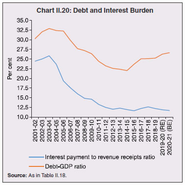
Table II.19: Composition of Outstanding Liabilities of State Governments and UTs
(As at end-March) | | (Per cent) | | Item | 2016 | 2017 | 2018 | 2019 | 2020 RE | 2021 BE | | 1 | 2 | 3 | 4 | 5 | 6 | 7 | | Total Liabilities (1 to 4) | 100.0 | 100.0 | 100.0 | 100.0 | 100.0 | 100.0 | | 1. Internal Debt | 72.1 | 73.3 | 72.7 | 72.2 | 73.4 | 74.9 | | of which: | | | | | | | | (i) Market Loans | 46.6 | 48.2 | 51.4 | 53.5 | 57.2 | 60.4 | | (ii) Special Securities Issued to NSSF | 17.5 | 14.0 | 11.1 | 9.2 | 7.7 | 6.3 | | (iii) Loans from Banks and Financial Institutions | 4.3 | 5.2 | 4.9 | 4.8 | 4.6 | 4.5 | | 2. Loans and Advances from the Centre | 4.7 | 4.1 | 3.8 | 3.6 | 3.4 | 3.3 | | 3. Public Account (i to iii) | 23.1 | 22.5 | 23.5 | 24.1 | 23.0 | 21.7 | | (i) State Provident Funds, etc. | 10.8 | 10.5 | 10.3 | 10.2 | 9.7 | 9.3 | | (ii) Reserve Funds | 4.3 | 3.2 | 4.1 | 4.2 | 4.3 | 4.1 | | (iii) Deposits & Advances | 8.0 | 8.8 | 9.1 | 9.7 | 8.9 | 8.3 | | 4. Contingency Fund | 0.1 | 0.1 | 0.1 | 0.1 | 0.1 | 0.1 | RE: Revised Estimate. BE: Budget Estimate.
Source: Same as that for Table II.18. | Composition of Debt 2.48 Outstanding debt, largely dominated by market borrowings, is expected to reach 75 per cent of GDP at end-March 2021 (Table II.19). There is a compositional shift towards market borrowings after the recommendation of the FC-XIV, to exclude states from National Small Savings Funds (NSSF) financing facility. Accordingly, the share of NSSF, bank and financial institutions and loans from the central government has been declining. Contingent Liabilities of States 2.49 Along with higher borrowings and the attendant servicing costs, debt sustainability of states is vulnerable to risks arising out of potential realisation of contingent liabilities in the form of guarantees, which have increased post COVID-19 (RBI, 2019a). As part of first tranche of the centre’s Aatma Nirbhar Bharat Package announced in May 2020, emergency liquidity infusion of ₹90,000 crore for cash-stressed power distribution companies (DISCOMs) was announced against state government guarantees, thus, adding to their contingent liabilities for 2020-21 by about 0.42 per cent of GDP (Table II.20)17. It may be noted that historically, any large accretion to states’ outstanding guarantees has, in general, been followed by an increase in debt. State guarantees, which increased prior to 2014, fell sharply thereafter, primarily driven by subsuming of power sector guarantees into state government liabilities under the UDAY programme. However, since 2017-18, net accretion to guarantees has seen a significant jump. This could be an early sign of future fiscal risks. Although a cap/ limit amounting to about 2 per cent of GSDP is considered optimal as per State Acts, there is no strict adherence to it. | Table II.20: Guarantees issued by State Governments | | Year | Guarantees Outstanding | Accretion during the Year | | ₹ lakh crore | In per cent of GDP | ₹ lakh crore | In per cent of GDP | | 1 | 2 | 3 | 4 | 5 | | 2013-14 | 3.79 | 3.4 | 0.80 | 0.4 | | 2014-15 | 4.28 | 3.4 | 0.49 | 0.1 | | 2015-16 (UDAY year) | 3.64 | 2.6 | -0.64 | -0.8 | | 2016-17(UDAY year) | 3.12 | 2.0 | -0.52 | -0.6 | | 2017-18 | 4.30 | 2.5 | 1.18 | 0.5 | | 2018-19 | 5.38 | 2.8 | 1.08 | 0.3 | | 2019-20 Provisional * | 6.00 | 3.0 | 0.62 | 0.2 | | 2020-21 (as per fiscal package)** | | | 0.90+ | 0.42+ | Note: * Based on actual reported for 20 states and last year’s value for balance states.
** States’ own guarantees given to SPSEs available only for few states as given in Statement 28.
Source: State governments. | 2.50 Even post-UDAY, state owned enterprises in power distribution (DISCOMs) continue to impart significant downside risk (leading to higher states’ liabilities) with no visible signs of turnaround. States’ outstanding liabilities increased by 1.5 per cent of GDP due to UDAY in 2015-16 and 2016-17; however, despite this steep fiscal cost, DISCOM losses since then have reached pre-UDAY level of 0.3 per cent of GDP in 2018-19. In fact, adjusted for revenue grants made under UDAY - which are transitory and in the nature of accounting transfers - DISCOM losses are significantly higher in 2018-19 vis-a-vis 2015-16 (Chart II.21a). Estimates of the revenue gap per unit of power sold - average cost of supply minus average realisable revenues (ACS-ARR gap) for 2019-20 reveal that most states have seen a further worsening in their financial performance. Only five states - Assam, Goa, Gujarat, Haryana and Maharashtra - have eliminated revenue gaps in 2019-20, thus meeting the UDAY target. Jammu and Kashmir, Rajasthan, Andhra Pradesh and Telangana have the highest revenue gaps, which have widened further in 2019-20 (Chart II.21b). 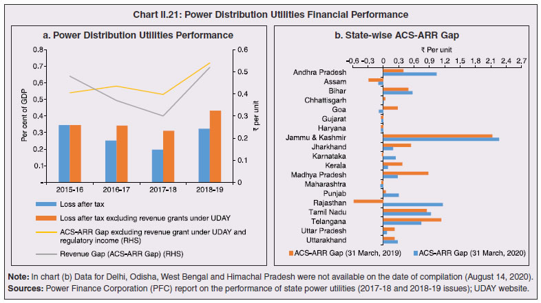 2.51 The financial position of DISCOMs is expected to weaken further in 2020-21 as COVID-19 related lockdown has severely impacted power demand, particularly in the lucrative industrial and commercial segments, while their cost structure is rigid due to minimum commitments for power offtake in long-term Power Purchase Agreements (PPAs). Structural issues remain to be addressed. While Union Government announced a liquidity support of ₹90,000 crore for DISCOMs which may help tide over immediate liquidity concerns, another round of bailouts of loss-making DISCOMs seems imminent in the aftermath of the crisis, imparting downside risks to state finances. 2.52 Going forward, managing fiscal risk through well laid down strategies is going to be critical, especially with emergence of new shocks and risks viz., the global financial crisis, natural calamities and now the pandemic. The fiscal risks could be (i) general, i.e., cyclical slowdown, macroeconomic shocks, commodity price shocks, interest rate shocks, and (ii) specific i.e., emanating from government guarantees and contingent liabilities and state-owned enterprises. In fact these specific fiscal risks have been observed to have disrupted efficient fiscal management leading to large debt spikes over the last decade (Jaramillio et al, 2017; IMF, 2017; Hemming, 2006). Similarly, severe problems in state-owned enterprises may underwrite economic slowdown and recessions, thus, necessitating large bailouts from the government - recent examples being Brazil and South Africa (IMF, 2020b). Given the lack of transparency with regard to states in reporting of some of these risks, efforts by Odisha in acknowledging, assessing and preparing in advance for such unforeseen risks could be worthy of emulation (Box II.4). Box II.4: Assessing Fiscal Risks – Odisha’s Experience The Government of Odisha identified “Fiscal Risk Management” as one of the key reforms priority under technical assistance from the IMF’ South Asia Regional Training and Technical Assistance Center (SARTTAC) in 2019. A dedicated Fiscal Risk and Debt Management Cell in the Finance Department and a high-level Fiscal Risk Committee has been put in place. The state has adopted a three-stage approach to fiscal risk management: (1) identification and measurement of fiscal risks; (2) fiscal risk reporting; and (3) mitigation and management of fiscal risk. Under (1), all possible sources of fiscal risk were identified and the impact of each fiscal risk worked out as ratio of GSDP and classified as high, medium and low on the basis of the level and possibility of occurrence (Chart 1a)18. Some of the identified sources of fiscal risk include (a) macroeconomic performance, international commodities prices, and exchange rate risk, particularly for foreign currency loans; (b) natural disaster to which Odisha is prone; (c) composite debt risk measured through a debt index consisting of debt to GSDP ratio, per capita debt and cost of debt using the relative distance methodology; (d) overall fiscal risk measured through a fiscal performance index employing a multiple indicator approach; and (e) contingent liabilities risk from Guarantees, Public Private Partnerships (PPPs)19, and public sector undertakings (PSUs). The state government also uses the IMF’s State-Owned Enterprise Health Check Tool to assess the financial health of the State PSUs. Such assessment of GRIDCO, a state-owned enterprise in power sector shows it a high risk company (Chart 1b). 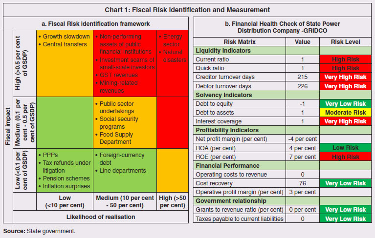 Fiscal risk reporting, critical for transparency and public disclosure, is envisaged through a two-stage approach. First, a Fiscal Risk Register as part of the Mid-year Fiscal Strategy Report identifying the sources of fiscal risks, risk exposure and likelihood and severity of risk materialization is put in place (Chart 2). Second, a Fiscal Risk Statement to be released along with Annual Budget documents would incorporate all possible fiscal risks for the state in quantified terms. This statement would be a part of the disclosure that the government intends to bring out, starting from the financial year 2021-22. 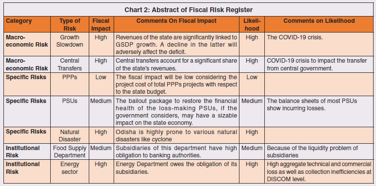 Mitigation and Management of Fiscal Risk is the third aspect as part of which a high level Fiscal Risk Committee headed by the Secretary, Finance was set up by the state government. It has already put in place mechanisms for management and mitigation of some of the major fiscal risks such as creation of State Disaster Response & Mitigation Fund (SDRMF), an administrative ceiling on government guarantees and constitution of a Guarantee Redemption Fund (GRF) for the fiscal risks arising from government guarantees and institution of a Consolidated Sinking Fund (CSF) to mitigate fiscal risks arising from amortization and foreign currency fluctuations. Over the years, the Government of Odisha has built up a sizeable CSF (about 15 per cent of state government liabilities) and GRF (about 25 per cent of total guarantee exposure). As a part of fiscal risk management measure for COVID-19 crisis, the state would utilise a portion of the CSF for amortisation of the entire open market borrowing during 2020-21. Going forward, the state intends to broad-base coverage of these funds and use them to address likely fiscal stresses in future. | 8. Conclusion 2.53 There are some specific features of states’ budget outcomes which are noteworthy. First, fiscal rectitude is reflected in large-scale pro-cyclical spending, making them vulnerable to downturns. Second, increased financing of fiscal deficits with market borrowings has pushed up debt levels, which may lead to tightening of debt servicing constraints. 2.54 Going forward, with states in the frontline in the battle against COVID, the fiscal arithmetic for 2020-21 is likely to suffer. While the focus during the first few months of 2020-21 has been on managing the health crisis, it is the regional and spatial dimensions of structural features like demography, health care systems, migrant workers, digitisation and strength of the third tier which are likely to play an important role going forward in determining the fuller macroeconomic impact of the pandemic on state finances.
|