Press Release RBI Working Paper Series No. 10 Are Food Prices Really Flexible?
Evidence from India GV Nadhanael* Abstract @This paper revisits the notion of flexibility of food prices by compiling a novel micro level dataset for India. It shows that food prices in India exhibit varying degrees of price stickiness across product groups. Furthermore, the price setting behaviour broadly matches predictions of sticky price models with menu cost. Model calibration shows that differences in productivity processes, market power and menu costs could account for the differences in price stickiness across product groups. Inflation based on a stickiness re-weighted food price index does not perfectly align with the conventional core measure of inflation (i.e., CPI excluding food and fuel). This highlights why paying attention to the sticky component of food inflation – besides core inflation – is important for the conduct of monetary policy in India. JEL Classification: E31, D40, C23 Keywords: Price setting, sticky prices, food prices, time-dependent pricing, state-dependent pricing Introduction Food prices are generally considered to be flexible. Driven by frequent supply shocks, food prices also exhibit large volatility. Monetary policy based on a New-Keynesian sticky price framework would then require that the relevant measure of inflation should abstract from such price changes. Therefore, a measure of inflation excluding food and fuel (referred to as core inflation), is usually considered as an appropriate target for monetary policy (Mishkin, 2008; Aoki, 2001). The notion of flexible food prices, however, has not been subject to much empirical scrutiny. Most of the empirical estimates of price stickiness did include food prices in their list of items but the focus was on estimating the aggregate measure of price stickiness. Klenow and Malin (2010) provide a summary of this literature. This study looks at price-setting behaviour within the food sector both from a macro and micro perspective in an emerging economy context, where, dynamics of food prices matter much for policy. Specifically, we ask the question: are food prices really flexible as commonly assumed or do we find evidence of price stickiness within the food sector? If so, does their behaviour align with the existing theories of price stickiness and what are the implications for policy? These questions assume importance in the background of recent developments in the literature on understanding the extent and role of price stickiness for policy. While initial works focused on a single parameter of price stickiness, Nakamura and Steinsson (2010) show that the heterogeneity in the degree of price stickiness across product groups raises the degree of monetary non-neutrality. Also, Kehoe and Midrigan (2015) argue that distinguishing between temporary and more permanent price changes is necessary to understand the role of price stickiness in monetary policy transmission. Therefore, this study accounts for both heterogeneity across products and the difference between temporary and permanent price changes in assessing price stickiness. In order to accomplish these tasks, this study has compiled a dataset on retail prices using the information available from the Price Information System set up by the Government of India. The compiled dataset comprises of 1.3 million price data points covering 45 food items on a weekly basis across 85 centres in India for the period 2005-18. This is one of the first attempts at compiling actual price data for estimating price stickiness in India. These products represent more than two-thirds of the items in the official CPI of food category representing each of the 10 product sub groups. Weekly frequency and wider geographical coverage lend the opportunity to have a better identification of price flexibility, especially in those items with very frequent price changes as compared with monthly data (Cavallo, 2018). The choice of India for this study is motivated by the fact that the degree of stickiness in food prices has more relevance for policy in India as food accounts for about 46 per cent in overall consumer price index (CPI), the highest among inflation-targeting countries. Therefore, the risk of policy errors from excluding sticky components, if any, in the food sector is larger in India as compared with advanced economies, where food has a low share in CPI (typically less than 10 per cent). Also, food price inflation showed considerable variability in India during the sample period (ranging between an annual average of 1.5 per cent in 2017-18 to 12.4 per cent in 2009-10) which gives us an opportunity to understand the degree of price stickiness in an environment of high variability in inflation. So far, most of the empirical work on price stickiness, with the exception of Gagnon (2009), was done in the context of developed countries, where the variability in inflation is generally low. Moreover, the food sector in India is also documented to have a market structure which is far from perfect competition. Chatterjee (2017) estimates significant market power for intermediaries in the food market in India while Banerji and Meenakshi (2004) document evidence of collusion among suppliers. Monopolist tendencies in the food market, therefore, provide a further case for understanding the price stickiness from a New-Keynesian point of view. Finally, though India adopted flexible inflation targeting as the framework for monetary policy in 2016, there exists limited studies on the extent of price stickiness using micro price data in India, a critical parameter for calibrating monetary policy models. Notably, Banerjee and Bhattacharya (2017) using sub-group level price indices for CPI for industrial workers (CPI-IW) obtained from Labour Bureau find greater monthly frequency of price changes and lower duration of price spell for food group, compared to non-food group. After controlling for small price changes due to sector-specific idiosyncratic shocks, stickiness in price-adjustment increases drastically for food components, corroborating to the high inflation persistence observed in the food sector in India. They also find evidence of sector-specific menu-cost driven pricing behaviour in India. This paper extends the literature by exploring a new micro-level actual price data as against price indices used in Banerjee and Bhattacharya (2017) to re-validate the price-stickiness of food prices in India. The paper starts with documenting the extent of stickiness of food prices in India. In terms of posted prices1 the median duration of a price spell2 is 1.3 months, which is somewhat longer than in the Banerjee and Bhattacharya study. However, there is large heterogeneity between product groups as it varies between half a month for vegetables to more than 5 months for milk. Following the methodology used by Eichenbaum et al. (2011), we then estimate an underlying price -the reference price- for each of the items as the price which occurs most number of times (mode) within a given quarter to assess the stickiness of permanent component of prices3. In terms of reference prices, the median duration increases to 4.3 months and the product level heterogeneity continues to persist with milk prices having a duration of more than 9 months. These results, therefore, do not support the hypothesis of food prices being completely flexible. This study also presents a set of stylised facts in line with Nakamura and Steinsson (2008) which characterise the price-setting behaviour. Decomposing total variation in the frequency of price changes across products into within and between components, we show that across product groups variation contributed to 82 per cent of the variation. We also find that prices are downward flexible with more than 40 per cent of the recorded price changes being price declines, even though aggregate food inflation remained positive for most of the time period. In terms of the size of price change, it varies between 5 to 19 per cent across product groups and the absolute size of price decreases, on an average, is marginally higher than that of increases. Over time, the frequency of price change co-move with aggregate food inflation. Many products also exhibit seasonality in the frequency of price changes. Spatially, perishable items show much larger variability in price levels across regions. Also, the frequency of price changes varies considerably across regions with northern and north-eastern regions showing a lower frequency of price change. These patterns point towards the importance of both product and region level factors in conditioning price-setting behaviour. The paper then provides evidence on how much the behaviour of food prices in India aligns with testable predictions of models of pricing in the literature; both state and time dependent4. First, we check for perfect staggering of frequency of price changes over time, a prediction of pure time-dependent pricing (Dias et al., 2005). We reject the hypothesis of perfect staggering of frequency of price changes and find that the frequency of price change is synchronized, both at the product as well as the centre implying that the frequency of price change is endogenous. In order to investigate the nature of state-dependency in a cross-section setting, we then look at the relationship between the size and the frequency of price change. This could either be negative or positive depending on the nature of menu costs (fixed or variable) and the type (temporary versus permanent) of cost and demand shocks (Berka et al., 2011). When shocks are transient and small, this relationship is negative if menu costs vary across firms. In the case of permanent and large shocks driving price changes, this relationship will be positive. The results show that for posted prices, the relationship between the size and the frequency of price change is ambiguous whereas for reference prices it is positive and significant. This suggests that the reference price changes are influenced by the permanent shocks whereas the posted prices are driven by transitory shocks. Theory predicts that the frequency and size of price change should be responsive to marginal cost changes over time in a state-dependent set up (Eichenbaum et al., 2011). We test this prediction using inflation as a proxy for marginal cost changes. For posted prices, frequency of price increase responds positively while the frequency of price decrease responds negatively to inflation. At the aggregate, they cancel each other out leading to no significant response of overall frequency of price change to inflation. Reference prices react in the same direction as posted prices but show greater responsiveness. However, a stronger positive response of frequency of price increase outweighs the negative response of frequency of price decrease leading to a positive and significant relationship between overall frequency of price change and inflation in reference prices. In terms of the size of price change, only the size of price decline responds negatively to inflation in case of posted prices. For reference prices, the size of increase responds positively and that of decrease responds negatively to inflation. These findings suggest that price-setting behaviour in food exhibit properties of state dependency where menu costs are important. Given the reduced-form evidence on state-dependent pricing, we then calibrate a standard menu cost model to see whether the standard menu cost models can generate the price-setting behaviour evident in the data. The calibration results show that the price-setting behaviour in the aggregate can be matched by a standard menu cost model and the model reasonably tracks the transition between high and low inflation periods. Calibrating the model at the sectoral level, we then show that differences in productivity and menu costs can account for the differences in price-setting behaviour across product groups. Finally, we look at the implications of the estimated price stickiness in food for policy. A measure of sticky food prices is generated by re-weighting the official CPI with the degree of stickiness. Inflation in the sticky components of food prices remained above the inflation excluding food and fuel during the high inflation phase and subsequently fell below as inflation moderated. This dichotomy implies that focusing only on inflation excluding food and fuel as a measure of underlying inflation entails the risk of policy errors by neglecting the dynamics of sticky components of food inflation. The rest of the paper is organised as follows. A discussion on contribution to literature is given in Section II. Section III describes the data used in the study and also provides definitions of various measures of price stickiness. In Section IV, we document the stylised facts with respect to food price setting in India and provide estimates of price stickiness for posted and reference prices. Reduced form estimates of theoretical predictions from pricing models are provided in Section V. Section VI discusses the model and calibration results. Section VII compares inflation derived from a sticky measure of food prices to that of overall food prices and core (excluding food and fuel) prices. Finally, in Section VIII, we offer the concluding remarks and sketch out possible areas for further research. II. Contribution to the Literature This paper contributes to the existing literature in the following dimensions. First, this study extends the literature on empirical estimation of price stickiness in line with the works of Bils and Klenow (2004) and Nakamura and Steinsson (2008) by providing a set of stylised facts for India, an emerging economy. The study also documents evidence for heterogeneity in price stickiness being driven by product group characteristics and regional variation of price stickiness within the same country which adds to the literature in terms of new stylised facts. Testing the empirical validity of time and state-dependent pricing models in the context of a developing country is another contribution of this paper. Klenow and Kryvtsov (2008) attempt to calibrate both time-dependent and state-dependent pricing models to test for empirical regularities of these models and find that both types of models exhibit empirical shortcomings even though state-dependent models enjoyed greater success. Other studies which particularly look at a specific sector or product include Cavallo (2018), who uses scrapped data from online retailers in five countries and Berka et al. (2011) who study price stickiness in online food prices in the case of a supermarket in Switzerland during a period of negative inflation. Evidence of state dependency in prices is also in conformity with theoretical literature and evidence for advanced economies (Golosov and Lucas, 2007). Regression results presented in the study provide further evidence on the mechanism by which responsiveness of frequency of price changes varies between posted and reference prices. We show that the frequency of price increases respond much more strongly in the case of reference prices. This drives the significance of response of frequency of price change to inflation in case of reference prices. Also, this work is one of the first attempts to calibrate a menu cost model to match the properties of price setting in the context of an emerging economy. Another dimension in which the paper adds to the existing literature is on understanding the role of food prices in monetary policy. Anand et al. (2015) show that under incomplete markets setting, changes in prices in the food sector could create demand effects from relative price induced income effects, and therefore, headline inflation targeting is the optimal policy. Catao and Chang (2015) characterise food prices as an important channel of transmission of commodity price shocks to the domestic economy. This study presents evidence for the existence of price stickiness of different degrees across different food product groups in India which in itself becomes a reason for explicitly taking into account the dynamics of food prices. This assertion follows from the findings of Eusepi et al. (2011) and Mankiw and Reis (2003) who show that the optimal monetary policy would have to assign weights proportionately to the degree of price stickiness. The paper, thus, makes a pioneering attempt to generate a stickiness re-weighted food inflation to show that conventional core inflation measures do not necessarily capture the dynamics of sticky food prices. III. Data and Measurement of Price Stickiness III.1. Data Currently, the National Statistical Office (NSO) of the Government of India releases only the item level price indices aggregated at the national level and no information about the actual level of prices is available. The Labour Bureau of Government of India releases average prices at item-level across 78 centres in the country which goes into the compilation of CPI for Industrial Workers5. These prices are not for identical products and also the price information is aggregated at the centre level. Therefore, using the price data which forms part of CPI has its limitations given the primary objective of understanding the extent of price stickiness. Given the inadequacy of the official CPI data, we use the data on prices available from the Price Information System set up by the Department of Agriculture and Co-operation, Government of India6. The system was set up for monitoring the retail prices of essential commodities in different parts of the country on a weekly basis. The retail prices7 are collected in respect of 45 food items that cover the broad spectrum of the consumption basket. Some of the items have prices quoted for more than one variety leading to a total number of 49 products/varieties for which prices are available. This covers 30 per cent of all India CPI and 65 per cent of the items covered within the food category of CPI. Appendix A lists the number of items along with their weight in overall CPI. The geographical coverage of this data is extensive with data reported from 85 centres spread all over the country. Prices are collected by using a proforma where a single price quote is obtained for each of the products from each centre. Various nodal agencies work as the agents of price collection which include Market Intelligence Units, State Government’s Bureau of Economics and Statistics, Agriculture Producing Market Committee (APMCs), District Supply Offices, Agriculture Marketing agencies, etc. Each week, the proforma is received by post by the central agency. Consistency is ensured by making sure that the prices are received for the identical item from all the centres by specifying the exact variety. The agency also makes sure that the reporting is regular by sending fortnightly reminders in case of missed reporting and also seeking clarifications from the data supplying agencies if the received data has a variation of more than 10 per cent. The data is compiled and disseminated in the ';Retail Bulletin of Food Items'; which is published every week. Part of this data is also hosted on the Ministry of Agriculture, Government of India website. We compiled this data using both the Weekly Bulletin and data hosted on the government website. Although the data is available from 2001, the reporting was quite irregular and data is available only for a few centres. Observation of the compiled data as well as discussions with the government officials revealed that the regular reporting of data started from 2005. Therefore, for the purpose of analysis, we use the data from the first week of January 2005 to the last week of March 2018 (a total of 691 weeks). The total number of price records are 1.3 Million, spread across 49 products/varieties and 85 centres. Data consistency was ensured by manually checking for reporting errors like zero coding of missing observations as well as errors in decimal points. Since the database is survey based, there could be a possibility of reporting error which could remain even after the checks are carried out. To make sure that minor errors in data entry as price changes are not included, we exclude all price changes which are denominated as less than 50 paise8 for price levels below 100 rupees and below 1 rupee for prices above 100. This filtering leads to the dropping of a marginal amount of price changes from the data (about 2400 from 1.14 million change observations). In order to ensure data robustness, Appendix B gives a number of checks to ensure that the results are not biased on account of missing observations and unbalanced nature of the panel. Moreover, to specifically address the question of whether more than 10 per cent variation is reported in the data, Appendix G plots the percentage change distribution of prices for a few select items to show that such a cut off for explanation does not lead to bunching of prices at that level. III.2.Measuring Price Stickiness There are two different approaches towards measuring price stickiness. The direct measure of price stickiness is the duration of a price spell which is the amount of time elapsed between two price changes. Counting the number of price spells in the data and taking the average of the observed durations can give the measure of price stickiness. This method, however, has two important limitations. First, the sample period is fixed, and therefore, observed price spells are truncated both at the beginning and end of the sample which could create bias in the estimation of duration. Secondly, in the presence of missing data, which is a case in the dataset used in this study, some restrictive assumptions will have to be made about the unobserved data points. Most empirical works on price setting, therefore, use the frequency approach, which is an indirect method of estimating the duration of price spells which we also follow. Price for a specific item in a single local market/store in a centre is denoted as Pict, where i, c and t stands for product, centre and week, respectively. For each product, the frequency of price change is computed as This gives the fraction of price observations at time t which were different from t−1 over all the observations for which prices at t and t−1 were observed summed across both centre and weeks. Similarly, we calculate the frequency of price increase and price decrease as The inverse of Fchangei would be a broad approximation of the duration of price spells. However, if we assume that prices could change at any point of time, in a continuous time set up, the duration of a price spell for a commodity is estimated as9 Once the duration at the product level is estimated, for arriving at measures of duration at product group and aggregate (all products) levels, we use product-level weights obtained from all-India item level CPI (Base: 2012). These weights are based on the all-India Consumer Expenditure Survey conducted in 2011-12. The products in the dataset are classified into 10 different product groups by matching each item with the corresponding group in CPI to which the item belongs to. Throughout this paper, duration estimates are converted to monthly frequency to make comparisons across reference periods and studies undertaken in other countries easier. The approach of using the observed frequency of price changes to understand price stickiness is not devoid of limitations. One of the major challenges is to distinguish between a mean-reverting temporary price change and a permanent price change driven by underlying demand or cost conditions. We partly address this issue in our discussion of posted versus reference prices in the following session. | Table 1: Behaviour of Food Prices in India: A Snapshot | | Product Category | Frequency of Price Changea | Duration (Months) | Proportion of Price Increasesb | Size of Change (%) | Size of Increase (%) | Size of Decrease (%) | Std. Dev. (Log Prices) | Obser-vations | | (1) | (2) | (3) | (4) | (5) | (6) | (7) | (8) | (9) | | Vegetables | 0.39 | 0.48 | 0.51 | 19.6 | 19.7 | 19.6 | 0.32 | 109342 | | Pulses and Products | 0.28 | 0.72 | 0.52 | 5.4 | 5.5 | 5.3 | 0.13 | 183319 | | Fruits | 0.25 | 0.84 | 0.53 | 15.1 | 14.8 | 15.6 | 0.34 | 50500 | | Sugar and Confectionery | 0.23 | 0.88 | 0.51 | 5.0 | 5.2 | 4.7 | 0.09 | 54343 | | Egg | 0.21 | 0.96 | 0.53 | 9.5 | 9.6 | 9.4 | 0.18 | 25156 | | Meat and Fish | 0.21 | 1.04 | 0.54 | 10.2 | 10.1 | 10.3 | 0.33 | 86945 | | Oils and Fats | 0.18 | 1.27 | 0.57 | 4.8 | 4.9 | 4.7 | 0.18 | 134332 | | Spices | 0.09 | 2.83 | 0.57 | 13.8 | 13.9 | 13.7 | 0.30 | 122540 | | Cereals and Products | 0.13 | 3.35 | 0.58 | 7.2 | 7.1 | 7.3 | 0.29 | 299266 | | Milk and Products | 0.04 | 5.13 | 0.7 | 9.1 | 8.7 | 10.1 | 0.16 | 71043 | | All Products (Median) | 0.16 | 1.34 | 0.55 | 6.9 | 6.9 | 6.9 | 0.24 | 1136786 | | All Products (Average) | 0.17 | 1.29 | 0.58 | 10.3 | 10.5 | 10.8 | 0.24 | 1136786 | | Source: Author’s calculations. a) Measured using equation (1). b) equation (2)/equation(1) | IV. Salient Features of Food Price Behaviour in India This section provides a set of stylised facts about the nature of price setting within the food sector in India. Since this study is the first attempt to characterise the nature of price setting in the Indian context, documenting these are important. Also, the patterns that emerge from these stylised facts throw light on the underlying factors conditioning price setting. These facts are reported in terms of (1) degree and price flexibility across products; (2) extent of downward flexibility; (3) size of price change; (4) spatial dispersion of price levels; (5) variation in price flexibility across time; (6) seasonality of price flexibility; and (7) regional variation in price flexibility. Table 1 summarises major indicators based on which these stylised facts are documented. We have also checked the sensitivity of these estimates to missing data and have found that they are robust (Appendix B). IV.1.Stylised facts IV.1.1. Food prices are flexible but with a significant level of heterogeneity On a weekly basis, the weighted median frequency of price change is about 0.16 which corresponds to a duration of 1.3 months. However, there is considerable heterogeneity across product groups. For example, vegetable prices on an average change about two times in a month whereas milk prices change only once in five months. Appendix C gives details of price behaviour across all the items covered in the study. Variance decomposition of product level frequency of price change indicates that between-group variation accounts for 82 per cent of the total variation10. The greater importance of product group level characteristics in conditioning price stickiness as against specific product-level factors could be on account of a number of reasons. Supply or sector-specific demand shocks could have similar effects on price stickiness of products within the same product group. Also, given the substitutability of products within the same product group, there could be spillover effects among products in a group creating a similar effect. Which of these channels dominates this phenomenon is an important question, but is beyond the scope of this paper. These results also throw light into the market structure in different product groups. For example, in the case of milk, we see that the prices are relatively sticky and the evidence suggests that the milk market in India is dominated by the co-operatives. Similarly for finished products like biscuit and bread we see a large duration of price spell. This is also indicative of the fact that at a higher end of the value chain prices tend to be stickier. The calibrated menu cost model in the subsequent section tries to address this issue explicitly. IV.1.2. Prices are flexible downwards for most products Most of the literature on price setting emphasises the role of downward price rigidity as a key driver of price stickiness. We find that prices are flexible downwards with an average of 42 per cent of the price changes being price decreases (45 per cent, if we use weighted median estimates). These estimates are similar to the ones derived for food prices in advanced economies viz. the USA, Euro area and Switzerland, which were in the range of 45 to 50 per cent (Klenow and Kryvtsov, 2008; Dhyne et al., 2006; Berka et al. 2011). As in the case of change frequency, we see considerable variation in this ratio across products. For select vegetables (tomato, onion and brinjal), price decreases are more frequent relative to increases (Appendix C). Nonetheless, aggregate inflation remained positive for each of these over the sample period for these items. This means that when prices increase, they increase by a larger magnitude. Milk and products, mutton and processed food items like biscuit and bread exhibited most downward rigidity with only less than 40 per cent of the price changes being price decreases. There exists a significant negative association between price flexibility (frequency of price change) and the ratio of price increases to total change observations (correlation coefficient of -0.82 between the two). Those food items which exhibit a longer duration of price spells are, therefore, the ones with relatively downward rigid prices. This, in fact, brings about the role of downward price rigidity in generating price stickiness. IV.1.3. Price change magnitudes are relatively large Column 5 of Table 1 gives the average size of absolute change in percentages, conditional on observing a price change. The average absolute size of a price change is about 10 per cent whereas the median price change is about 7 per cent on account of the positively skewed distribution of the absolute size of price changes. Vegetables and fruits have a high level of absolute price change of 19 and 15 per cent, respectively indicating that these prices are extremely volatile across time with the amplitude of price changes being very large. On an average, the absolute size of price decreases is marginally higher than that of price increases. At the product group level, however, we see a significant divergence in this pattern with only 4 of the 10 product groups having a higher absolute size of a price decrease. IV.1.4. There is considerable spatial variation in price levels across centres We computed the standard deviation of the logarithm of prices at the product level across all centres for each week. This was averaged for the entire time period to generate product level statistics. This was further aggregated by using a weighted sum within each product group using CPI weights and is reported in Column 6 of Table 1. On an average, for most of the relatively perishable items, like vegetables, fruits, meat, fish and spices, prices show much more cross-sectional variability as compared with more durable items like pulses, sugar and edible oils. Cereals and milk are, however, an exception to this general pattern. IV.1.5. Frequency of price change co-moves more with inflation than the size of price change To gauge the link between food price inflation and frequency of price changes, we look at the trends in change frequency (overall, increase and decrease; weighted average across products) against inflation in CPI for food items over the time period. To abstract from volatility in the frequency of price changes on a week to week basis and also to make sure that there are enough samples in each time period, a quarter is taken as the unit of analysis. For each quarter, the frequency of price changes and the absolute size of changes are estimated at the product level and then arrive at a weighted average for each of the product groups. Chart 1 plots the trends in the frequency of price changes over time. The overall frequency of price change remained range-bound between 15-20 per cent for most of the time-period, barring the latest few quarters (2017 onwards) when it fell below that range. The trend in annual inflation based on food category CPI for Industrial Workers (IW)11 is plotted in the secondary axis. The variability in the frequency of price change across high and low inflation episodes is of a lower magnitude than that of the change in inflation. The frequency of price increases and decreases move in the opposite direction to changes in inflation. Higher inflation is associated with a higher frequency of price increase whereas the frequency of price decreases co-moves negatively with inflation. Since the overall frequency of price change is a sum of these, they may cancel out each other leading to lower variability in the frequency of price change. The period since 2017, however, is marked by a decline in the frequency of price increase leading to a fall in the overall frequency of price change, something which can be expected in a low inflation environment. We also checked whether the decline was broad-based by looking at the trends in each of the product groups and the results indicated that both the decline in inflation and change frequency was indeed broad-based (Appendix D). 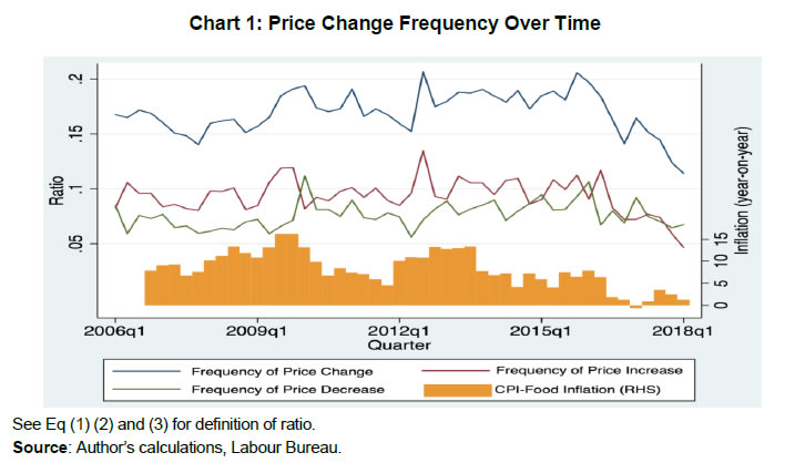
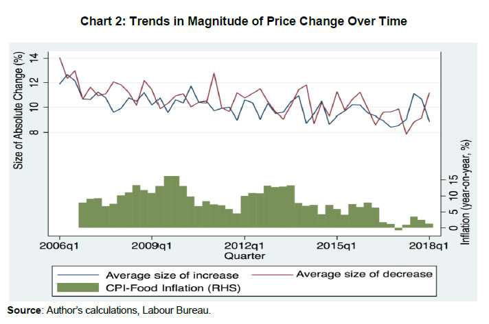 We also looked at the trends in the average absolute size of price change (both increase and decrease separately) over the sample period. Chart 2 indicates that the size of absolute change remained volatile but in a very narrow range of between 8-12 per cent for most of the time period. The CPI food inflation, however, ranged between -0.1 to 16.3 per cent during the same period. These results show that inflation is associated more with the frequency of price change than size. IV.1.6. There are Seasonal Variations in Price Changes Food prices in India exhibit significant seasonal patterns largely following the crop cycle. The co-movement of the frequency of price change with inflation that we observed above is translated into a seasonal pattern in price change frequency too. In Chart 3, we plot the average frequency of price increases and decreases across quarters. We see that the largest frequency of price increase and the smallest frequency of price decrease occurred in the April-June quarter. From thereon, there is a gradual decrease in the frequency of increase over successive quarters and for the frequency of price decreases, the trend is the opposite. This is largely driven by the seasonal pattern where the arrival of winter crops usually leads to a fall in prices. 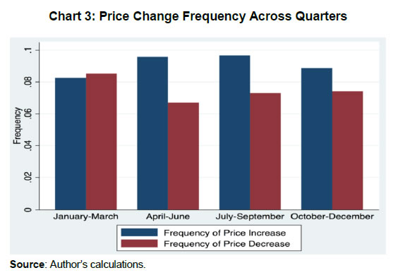 The seasonal pattern, however, is not uniform across different product groups. We estimated the seasonal effects on price change frequency as follows. For each of the product groups in the dataset, frequency of increase and decrease is regressed on the month of the year dummy variable keeping August as the base, a month usually devoid of unusual changes in prices. Data was aggregated at the centre level with centre fixed-effects incorporated in the regression. The coefficient of each month gives us an idea about whether the price increase/ decrease frequency was significantly different in that month as compared with the base month (August). Coefficients from individual regressions for each product group are reported in Appendix E for both frequencies of price increases and decreases. The key takeaway is that as compared to August, the frequency of price increases was generally lower for vegetables, pulses, sugar and spices during the period December to April. Except for spices, all of these also had a higher frequency of price decreases from December to March. Cereals and Milk, two of the product groups with the largest weight in CPI, however, do not exhibit much seasonality in the frequency of price changes. IV.1.7. Price stickiness varies across regions. The literature on price stickiness and spatial dispersion largely focuses on the role of sticky prices on generating price dispersion across the outlets in a homogeneous location (Kaplan and Menzio, 2015; Sheremirov, 2019). In this paper, we look at the dispersion in price stickiness across different regions in India. Different regions in India could be expected to have different characteristics in terms of price-setting behaviour owing to its diversity in the level of economic development as well as other factors like institutions and infrastructure. India can be classified into five different regions, North, South, East, West and North East12. The overall region-wise frequency of price increases and decreases are reported in Chart 4. We see that frequency of price changes is lower in the Northern and North-Eastern regions as compared with the other regions. 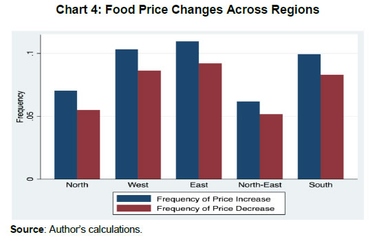 There could be a host of factors that influence the varying degrees of price stickiness across regions. Within the limited scope of this paper, we focus on two important economic characteristics and their association with the level of price stickiness across regions. Per-capita income can impact the demand elasticity of food and also stand for the level of economic development. We worked out the correlation coefficient between average per-capita income during the time period under the study (2005-17) across 27 states for which data was available and the degree of price flexibility. Per capita income at the state level and the frequency of price changes do not exhibit any significant co-movement (correlation coefficient of -0.08). Another important factor could be the level of infrastructure. If a region is well connected with the rest of the country, it could have a less severe impact from local supply shocks but is more prone to shocks in other regions. Also, in a region with poor connectivity changes in transport costs would have an impact on inflation as well as the frequency of price change. We calculated the correlation between price change frequency and rural road density per thousand population across various states. There exists a negative and significant correlation between price change frequency and rural road density (coefficient of -0.48 with a ‘p’ value of 0.01). The take away from these stylised facts is that the price setting in the food sector has a lot of heterogeneity and is conditioned by the type of the product, level of aggregate food price inflation, seasonal effects as well as spatial factors. All these indicate that the price setting is influenced by underlying economic conditions. IV.2. Price stickiness in low versus high-frequency price movements Estimating an appropriate degree of price stickiness is also dependent on the selection of the time frame. Initial works on empirical estimation of price stickiness, however, ignored this question. Bils and Klenow (2004) estimate price stickiness in the US taking into account all the price changes by arguing that even the magnitude and duration of temporary price changes are driven by shocks, and therefore, a realistic estimation of price flexibility should include those changes as well. Nakamura and Steinsson (2008) counter this and argue that some part of the sales could be orthogonal to underlying macroeconomic conditions, and therefore, needs to be excluded while estimating price stickiness. The result is that while Bils and Klenow (2004) found the duration of price spells to be 4.3 months, Nakamura and Steinsson (2008) estimate it to be at a much higher level of 7-11 months. This debate initiated a number of subsequent works that tried to reconcile the simultaneous existence of differential price stickiness at low and high frequencies. Kehoe and Midrigan (2008) show that firms could set prices separately for a shorter and longer horizon, under the assumption that temporary price changes are less costly than more permanent price changes. Eichenbaum et al. (2011) examine the impact of this on macroeconomic policy and conclude that the monetary policy has substantial real effects in the presence of differential price setting between temporary and reference prices. Kehoe and Midrigan (2015) extend both the standard Calvo pricing and menu cost models by adding separate frictions to show that low-frequency price movements do respond to monetary policy shocks. The empirical estimates for other countries also support the hypothesis of different price stickiness at high and low frequency (see Berka et al., 2011 for Switzerland). The case for looking at a low-frequency movement of prices, therefore, is stronger in the debate on the appropriate measure of price stickiness. Identifying the temporary price changes from the data and defining an appropriate time frame for low-frequency price movements are the two important challenges in estimating low-frequency price stickiness. Those studies which used the official CPI data from the US had the advantage of data collection agency recording a separate identifier for the sales price. In those datasets which do not have an explicit identification of the sales price, some excluded those price changes which revert to the original price in the next period while estimating the frequency of price changes. The other approach is to define a time frame for which a reference price could be set and then use the price which is recorded the most number of times within the reference period (modal price) as the reference price. The literature is rather ambiguous on the selection of time frame for calculating the reference price. Eichenbaum et al. (2011) justify the choice of the quarter as a reference time frame by stating that most macroeconomic models are calibrated on a quarterly basis and the nature of price movements is similar between monthly and quarterly reference time frames. Kehoe and Midrigan (2015) select an annual time frame as the reference period, which was justified by the fact that even at annual frequency, about 73 per cent of the posted prices were equal to the reference prices. Moreover, they also found that this ratio is consistent with the moments generated by the calibrated menu cost model in their study. Similarly, there is no identification of sales prices in our dataset, and therefore, defining a time period for calculating the reference price is the first challenge. Using a simple method of excluding price changes which revert within one period does not allow us to clearly identify the temporary price changes, given the level of flexibility that we observed in posted prices. For example, prices may rise by 10 per cent and subsequently fall by 2 per cent for five consecutive weeks for it to reach the original level. Excluding mean-reverting price changes would, therefore, be difficult in such a scenario. Changing the reference period may lead to a different estimate of the duration of price changes but the ranking of products in terms of the degree of price flexibility should be more or less similar irrespective of the time frame. For each of the time frames (weekly, monthly, quarterly and annual), the reference price is defined as the modal price. Subsequently, the Spearman rank correlation of estimated duration across each of these reference prices at the product level is worked out (Table 2). We see that the ranking of products according to the degree of price flexibility is maintained almost the same up to the quarterly frequency, whereas in annual frequency, the rank correlation coefficient falls markedly. Additionally, we calculated the fraction of prices that are equal to the reference prices in each of the time frames. For monthly and quarterly time frames, these fractions were 86 per cent and 74 per cent, respectively, while for annual frequency it fell to 54 per cent. These indicate that annual frequency may not be a true representation of the low-frequency price movements. Intuitively, agricultural price cycles in India could be expected to have less than the annual frequency as many crops have a shorter than annual crop cycle. Even many annual crops are cultivated more than once in a year (during kharif and rabi seasons). In view of these, we select a quarterly time frame as the period for calculating the reference price which is also informed by the fact that the fraction of prices at mode prices in quarterly estimates matches with the results from Kehoe and Midrigan (2015). | Table 2: Spearman Rank Correlation between Duration Estimates | | Time | Weekly | Monthly | Quarterly | Annual | | (1) | (2) | (3) | (4) | (5) | | Weekly | 1 | | | | | Monthly | 0.982 | 1 | | | | Quarterly | 0.943 | 0.983 | 1 | | | Annual | 0.733 | 0.807 | 0.875 | 1 | | Source: Author’s calculations. | We see that the duration increases significantly with quarterly reference prices. It increases from 1.3 months in the posted prices to 4.1 months with reference prices. Table 3 compares the duration estimated with quarterly reference price data with that of the posted price (weekly) estimates across all the major food product groups. The large dispersion in duration across product group continues to persist with the standard deviation of duration measured on quarterly reference prices being 4.48. The duration of reference prices in the case of cereals, spices and milk are in the range of 7-10 months, which is not in conformity with the notion of perfectly flexible food prices. Except for vegetables and pulses, posted prices are equal to reference prices for more than two-thirds of the sample indicating that for most product groups such reference prices are indeed relevant. We can, therefore, conclude that the notion of food prices being extremely flexible needs to be re-looked as there is evidence of a much higher level of price stickiness at low frequency. | Table 3: Duration Estimates based on Weekly and Quarterly Reference Prices | | Product group | Duration based on | | Weekly | Quarterly | % at Reference Price | | (1) | (2) | (3) | (4) | | Vegetables | 0.48 | 2.17 | 54 | | Pulses and products | 0.72 | 2.52 | 62 | | Sugar and Confectionery | 0.88 | 2.74 | 66 | | Fruits | 0.84 | 3.54 | 68 | | Egg | 0.96 | 3.54 | 69 | | Oils and fats | 1.27 | 3.85 | 73 | | Meat and fish | 1.04 | 4.42 | 73 | | Cereals and products | 3.35 | 7.04 | 78 | | Spices | 2.83 | 7.37 | 85 | | Milk and products | 5.13 | 9.52 | 91 | | Source: Author’s calculations. | How far our results align with evidence from other countries? Studies undertaken in different country contexts indicate that generally, food prices are much more flexible than non-food prices (Table 4). Also, in all the countries, food prices are more flexible in posted prices than in reference prices. Our estimate of posted price duration is lower than most studies in the literature. Estimates of reference price level duration in food prices in India, however, is higher than the corresponding number for the US reported by Nakamura and Steinsson (2008). | Table 4: Estimates of Duration of Price Spells (Months): Select Countries | | Country | Study | Food Prices | Overall | | Posted | Reference | Posted | Reference | | (1) | (2) | (3) | (4) | (5) | (6) | | US (Offline) | Nakamura & Steinsson (2008) | 2.1 | 3.5 | 4.6 | 11.0 | | US (Online) | Cavallo (2018) | | - | 4.3 | - | | Euro Area | Dhyne et al. (2006) | 3.0 | - | 10.6 | - | | Switzerland | Berka et al. (2011) | 2.2 | 37 | - | - | | Brazil | Gouvea (2007) | 1.6 | - | 1.9 | - | | India | This study | 1.3 | 4.1 | - | - | | Source: Author’s calculations, references as cited above. | Another important question is how relevant are these estimated levels of price stickiness for macroeconomic policy? Literature provides a comparative perspective on how these results line up with the theoretical postulates. The first generation of New-Keynesian macroeconomic models was in a single sector framework with one price stickiness parameter and most calibrated models used/estimated it to be in the range of 6-9 months (Smets and Wouters (2007) use 6 months while Christiano et al. (2005) and Gertler and Leahy (2008) estimate it to be 7.5 months). The median estimate of this study for food prices is lower than these. Smets and Wouters (2007), however, show that a reduction of price stickiness weakens the strength of nominal rigidities through an increase in the persistence of mark-up shocks and price indexation but does not eliminate it. Therefore, the real effects of nominal shocks in the food sector could still be relevant, though not as strong as the benchmark models. With respect to heterogeneity across product groups and the difference between stickiness in posted and reference prices, Golosov and Lucas (2007) show that in the presence of menu costs and strong state dependency in pricing, monetary non-neutrality becomes small and transient, which questioned the foundation of New-Keynesian macroeconomic policy. In response, Nakamura and Steinsson (2010) calibrate a multi-sector menu cost model with heterogeneity in frequency and size of the price change and show that accounting for heterogeneity in price-setting would increase the monetary non-neutrality by a factor of three. Further, Midrigan (2011) shows that distinguishing between temporary and permanent price changes would make the models in line with Golosov and Lucas (2007) that produce a similar level of monetary non-neutralities as in a standard Calvo pricing model. Our results show that both these factors are at work in the food sector in India, and therefore, there is a non-negligible role for food price stickiness in the policy. V. Models of Price Stickiness and Behaviour of Food Prices in India This section is devoted to understanding how far the observed characteristics of price setting in the food sector in India are driven by the identified reasons for price stickiness in the literature. Understanding this is important as the macroeconomic policy framework of inflation targeting is based on the assumptions of the presence of price rigidities working through the channels identified in the literature. Macroeconomic literature on price setting is broadly divided into time-dependent and state-dependent pricing models. In a time-dependent pricing model, the timing of price change is exogenous. If we assume that the underlying process is approximated by a Taylor (1980) set up, firms get to change the price in every nth period. Therefore, the proportion of firms changing their prices is constant across time. In a Calvo (1983) formulation, only a fraction of firms are able to reset their prices at any point of time and the probability of price adjustment is random. Even under the Calvo model of price setting, under the assumption of independent decision of price change by each firm, the expected value of proportion of firms changing their prices is constant over time (Klenow and Kryvtsov, 2008). This implies that the frequency of price change would be perfectly staggered under pure time-dependent pricing with the expected value of fraction of sellers changing their price being constant over time. In state-dependent pricing models, firms face a cost of changing the price (menu cost) and the decision to change price is dependent on the size of the marginal cost or demand shock and the extent of menu cost. One way to look at the empirical validity of state-dependent pricing is to see the relationship between the frequency of price change and its size in cross-section. This relationship could either be positive or negative conditional on the specifications/assumptions about the underlying process for menu costs and shocks to demand or cost faced by the firms. If menu cost differs across firms and they face mean zero independent and identically distributed (iid) shocks to cost/demand, we would expect a negative relationship between size and frequency of price change in cross-section. This is because, firms with large menu costs will wait longer to change their price (implying lower frequency) and accumulated costs would imply a larger size of price change (Berka et al., 2011). In the presence of large idiosyncratic shocks with a fat tail distribution, firms frequently hit their upper bound of the price change and they change their price more often and by a larger amount which generates a positive relationship between frequency and size of price change (Klenow and Kryvtsov, 2008). Also in terms of the dichotomy between the behaviour of posted price and reference price, Kehoe and Midrigan (2015) calibrate the model with both permanent and transitory idiosyncratic shocks to productivity. This enables them to match the differential response of posted and reference prices to the shocks. If the permanent shocks are large and persistent, we can expect the sellers to pass it on by raising both the frequency and size of price change leading to a positive relationship between the two in case of reference prices. Regression of the size and frequency of price change on marginal cost over time is another way to identify the extent of state dependency. The literature, however, does not have a consensus on either the magnitude of impact or on the relative importance of frequency and size of price change. For example, in response to a monetary shock, the average size of change responds to the shock in the model of Golosov and Lucas (2007) whereas in Dotsey et al. (1999) it is the fraction of firms who change their price which responds to the shock. We now examine how these predictions are borne out by the data. V.1. Staggering versus Synchronisation in Price Changes An empirical test for staggering versus synchronisation in price changes was proposed by Fisher and Konieczny (2000) while studying the price-setting behaviour of Canadian newspapers. They proposed the following measure: Where, N is the number of cross-section observations and T is the total time period which follows a χ2 distribution with (T−1) degrees of freedom. We use the same measure to test for perfect staggering in price setting. As price setting could be synchronised/staggered or both across centres and products, we conduct the test for perfect staggering both at the commodity level and the centre level. The null hypothesis of perfect price staggering both at the product level and the centre level is rejected. Appendix F gives the results of the test. The evidence of synchronisation at the centre level (prices of different commodities at the same centre) points towards centre specific state variables having a significant role in shaping price stickiness. A similar argument can be made with product-level synchronisation i.e., prices of the same product across different centres show evidence of synchronisation indicative of the importance of product level state variables too. If we take the value of FK index as the degree of price synchronisation, on an average, the value at the centre level is higher than the value at the product level. V.2. Relationship between Duration and Size of Price Change As discussed earlier, conditional on the nature of menu costs and the magnitude of cost or demand shocks, the relationship between size and frequency of price change could be either positive or negative. How this relationship is manifested in our data is tested by estimating the following regression in a cross-section set up. where Yic is the absolute size of price change and Xic is the frequency of price change for product i at centre c averaged across all time periods. γc and γp are centre level and product group level fixed effects. Since we have documented that there is significant heterogeneity in price-setting behaviour across different product groups, we also ran separate regressions on each of the product groups with the same specification but with only centre level fixed effects. There exists no significant relationship between the frequency of price change and size at the aggregate level if we look at the posted prices (Table 5). At the category level, cereals, oils, pulses, sugar and spices have a negative and significant relationship indicating that for posted prices variability in menu costs is likely the major contributor to differences in frequency of price changes in these items. Vegetables, however, have a positive and significant relationship between size and frequency of price change which could be on account of the fact that weather-related supply shocks are very frequent, creating large shocks to marginal costs impacting both frequency and size of price changes. In the case of reference prices, we see a positive and significant relationship between the size of the price change and frequency of price change both at the aggregate level and in all of the product groups. If we follow the argument of Kehoe and Midrigan (2015) that reference prices adjust to permanent component of shocks, and therefore, both the size and frequency of price changes respond to more permanent changes in marginal cost or demand. Posted prices showing an ambiguous or negative relationship when reference prices have a positive correlation indicates that transitory shocks are equally if not more important as they effectively undo the effects of permanent shocks. A full exposition of these dynamics, however, would be possible only with a state-dependent model calibrated with these specificities. | Table 5: Regression of Size of Price Change on Frequency: Dependent Variable: Average Absolute Size of Log Price Change | | Category | Posted Prices | Reference Prices | | Coefficient | Std. Error | Coefficient | Std. Error | | (1) | (2) | (3) | (4) | (5) | | All Products | -0.11 | (0.07) | 0.17*** | (0.04) | | Cereals and products | -0.46*** | (0.04) | 0.10*** | (0.01) | | Meat and fish | 0.03 | (0.03) | 0.23*** | (0.02) | | Milk and products | 0.10 | (0.17) | 0.06*** | (0.02) | | Oils and fats | -0.18*** | (0.04) | 0.06*** | (0.01) | | Fruits | -0.10 | (0.08) | 0.37*** | (0.03) | | Vegetables | 0.23*** | (0.04) | 0.66*** | (0.05) | | Pulses and products | -0.07*** | (0.01) | 0.09*** | (0.01) | | Sugar and Confectionery | -0.22*** | (0.06) | 0.12*** | (0.02) | | Spices | -0.54*** | (0.11) | 0.29*** | (0.04) | Note: * p<0.1, ** p<0.05, *** p<0.01.
Explanatory variable is the frequency of price change in all the regressions.
For all products, the regression includes centre and product group level fixed effects.
Standard errors are clustered at product group level. Estimates for egg is not reported as there is only one product in the category.
Source: Author’s calculations. | V.3. Response of Frequency and Size of Price Change to Inflation In a state-dependent pricing model, the response of frequency and size of price changes to marginal cost shocks is the major channel through which the variation in price stickiness over time can be identified. Empirical identification of this relationship is difficult as marginal cost is not directly observable in most cases. Eichenbaum et al. (2011) is the only exception where they could explicitly get the data on the movement of marginal cost as well as prices from the same dataset. Most of the other studies use some measure of aggregate inflation as a proxy for changes in marginal cost. Nakamura and Steinsson (2008) use the aggregate level of inflation, while, Dhyne et al. (2006) as well as Berka et al. (2011) use the regional and sectoral level inflation, respectively, as a proxy for marginal cost. Following the identification strategy in the literature, we use the CPI product group inflation as the proxy for marginal cost. All India CPI is available only from 2011, which restricts the analysis to only the period 2011-18. The trends in both year-on-year and month-over-month CPI inflation for food during this period shows that our sample period had considerable variability in inflation. As compared with the other studies in the literature, our empirical setting provides the scope for better identification as the period under our analysis is characterised by significant variability in CPI food price inflation. Also, from a methodological point of view, in most of the studies, annual inflation (log difference of 12 months) was used as a proxy for marginal cost. Changes in annual inflation, however, could be driven by base effect as much as price change in the latest period. For example, if there was a sudden fall in prices in last year in the same month, when we calculate the annual inflation, inflation could go up even when prices in the current period remain constant13. To overcome this potential bias, we use the first difference in log CPI. The basic specification is as follows,  Where, Yit is the variable of interest averaged across weeks and centres for a product i in a month/quarter t. There are five estimates with different dependent variables; frequency of price change, frequency of price increase, frequency of price decrease, absolute size of increase and absolute size of decline. Δlog(CPI)pt is the first difference of log of CPI for product group p in period t. γt are time fixed effects and γp are product group-level fixed effects. The presence of a large number of centres in the dataset enables us to follow such an identification strategy. We run the regressions both on posted prices are well as reference prices (quarterly mode). Table 6 reports the results for posted prices. | Table 6: Regression of Frequency and Size of Price Change on CPI Inflation (Posted Prices) 2011-2018 | | Dependent Variable | chf | incf | decf | abinc | abdec | | (1) | (2) | (3) | (4) | (5) | (6) | | ΔlogCPI | -0.05 | 0.93*** | -0.98*** | 0.01 | -0.19*** | | | (0.10) | (0.25) | (0.15) | (0.03) | (0.02) | | Product Category FE | Y | Y | Y | Y | Y | | Month FE | Y | Y | Y | Y | Y | | Adj R2 | 0.654 | 0.500 | 0.568 | 0.358 | 0.066 | | N | 4263 | 4263 | 4263 | 4187 | 4100 | Note: * p<0.1, ** p<0.05, *** p<0.01
Figures in parentheses are robust standard errors, clustered at product group level
chf: Frequency of Price Change, incf: Frequency of Price Increase
dncf: Frequency of Price decrease, abinc/abdec: Mean (absolute) size of increase/decrease
Source: Author’s calculations. | The coefficient of regression of frequency of price change (chf) on inflation is insignificant which may suggest that the price change frequencies do not respond to marginal cost shocks. However, under state-dependent pricing, the cost of changing price is compared with the size of marginal cost such that the seller would change the price when marginal cost is above menu cost. Therefore, when inflation is high, more producers are likely to revise their prices upwards and vice versa. Likewise, when there is an increase in marginal cost, the proportion of price decreases will fall. Therefore, we need to look at the frequency of price increases and decreases separately. The results reported in columns 3 and 4 of Table 6 show that the frequency of price increases (incf) respond positively to changes in inflation while price decreases (decf) respond negatively. Thus, it cancels out in the aggregate change frequency, which is a sum of these two, as the magnitude of response of both price increases and decreases are similar. Turning to the absolute size of price increases and decreases, absolute size of price increases does not respond to inflation whereas price decreases respond to it. This is intuitive as the sellers would not want to increase the size of the price increase and thereby lose customers whereas they can easily reduce the size of the price decline to accommodate the shock. If we look at the reference prices, the overall frequency of price change responds positively to inflation (Table 7). The pattern of frequency of price increases responding positively to inflation and price decreases responding negatively is maintained in the reference prices. | Table 7: Regression of Frequency and Size of Price Change on CPI Inflation (Reference Prices) 2011-2018 | | Dependent Variable | Chnfq | incfq | decfq | abinc | Abdec | | | (1) | (2) | (3) | (4) | (5) | | ΔlogCPI | 0.11**
(0.05) | 1.85***
(0.26) | -1.73***
(0.23) | 0.46***
(0.14) | -0.51***
(0.14) | | Product Category FE | Y | Y | Y | Y | Y | | Quarter FE | Y | Y | Y | Y | Y | | Adj R2 | 0.510 | 0.364 | 0.460 | 0.147 | 0.351 | | N | 1421 | 1421 | 1421 | 1410 | 1362 | Note: * p<0.1, ** p<0.05, *** p<0.01
Robust standard errors in parentheses, clustered at product group level.
chf: Frequency of Price Change, incf/ decf: Frequency of price increase/decrease.
abinc/ abdec: Mean (absolute) size of increase/decrease
Source: Author’s calculations. | The magnitude of coefficient increases significantly in both the cases, but more so for price increases. In terms of the size of price changes, now the size of price increases responds positively to inflation while the size of price decreases continues to respond negatively to inflation. Thus, in terms of the response of frequency and size of price change, reference prices show much more alignment with the predictions of a standard state-dependent model. VI. Calibrated Menu Cost Model In this section, a partial equilibrium menu cost model for food price data in India was calibrated14. The objective here is to use an existing standard menu cost model in a flexible price set up. In order to keep the model tractable, all the agents in the supply chain are combined as one entity which enjoys market power. While this is a simplification of the real-world supply chain network, the idea is to incorporate all the frictions in the entire supply chain and show that it matters for price setting. VI.1.Calibration The model is calibrated to match key attributes of the food price data on a weekly frequency. The targeted moments were frequency of price change, average size of the price change and proportion of price changes which increase. We follow the literature on picking the standard parameters. Using aggregate CPI for food inflation in India for the period of 2006-18, the value of μ and σμ are estimated on monthly data and the corresponding weekly frequency is worked out. Parameter values used in calibration are detailed in Table 8. | Table 8: Selection of Parameters for Calibration | | Parameter | Value | Choice Benchmark | | (1) | (2) | (3) | | Β | 0.96 | Literature | | Θ | 3 | Lower bound in the literature | | µ | 0.00138 | Estimated from CPI Food in India during 2006-18 | | σµ | 0.0063 | Estimated from CPI Food in India during 2006-18 | | Ρ | 0.7 | Calibrated | | σϵ | 0.05525 | Calibrated | | K | 0.0153 | Calibrated | | Source: Author’s calculations. | Table 9 reports the three major variables of interest from the data and the calibrated model. We see that once we match the frequency and size of price change, the proportion of price increases and the standard deviation of log prices also are matched by the model. These are generated from a price series of 250,000 observations simulated from the data. Standard deviations are on 700 weeks of data to avoid the scale effects and also to match the time frame in the sample. | Table 9: Comparing moments between the data and the model | | Variable | Data | Model | | (1) | (2) | (3) | | Targeted Moments | | | | Frequency of Price Change (%) | 19.0 | 19.0 | | Average Size of Price Change (abs) (%) | 10.49 | 10.51 | | Fraction of Price Increases (%) | 54.0 | 54.7 | | Non-targeted moments | | | | Std.Dev of Log Prices | 0.24 | 0.27 | | Size of Price Increases (%) | 10.36 | 10.32 | | Size of Price Decreases (abs)(%) | 10.66 | 10.73 | | Source: Author’s calculations. | VI.2.Disaggregated Analysis The data has two distinct episodes of food price inflation in India. For a decade between 2006 and 2016, on average, food prices grew at a rate of about 10 per cent. Since then, inflation in food prices has been below 2 per cent. We now recalibrate the model to look at how far the model can account for the change in inflation regime in terms of the properties of the data. Here, we only change the aggregate food inflation mean and variance (μ and σμ) and keep the rest of the parameters same as a benchmark case. | Table 10: High inflation period: data and the model | | µ = 0.0018 and σµ = 0.006682 | | Variable | Data | Model | | (1) | (2) | (3) | | Targeted Moments | | | | Frequency of Price Change (%) | 19.74 | 19.77 | | Average Size of Price Change (abs) (%) | 10.46 | 10.46 | | Fraction of Price Increases (%) | 55.4 | 55.2 | | Non-targeted moments | | | | Std.Dev of Log Prices | 0.25 | 0.31 | | Size of Price Increases (%) | 10.30 | 10.30 | | Size of Price Decreases (abs)(%) | 10.67 | 10.66 | | Source: Author’s calculations. |
| Table 11: Low inflation period: data and the model | | µ = -0.0002 and σµ = 0.006612 | | Variable | Data | Model | | (1) | (2) | (3) | | Targeted Moments | | | | Frequency of Price Change (%) | 16.4 | 18.6 | | Average Size of Price Change (abs) (%) | 9.24 | 10.49 | | Fraction of Price Increases (%) | 46.3 | 51.0 | | Non-targeted moments | | | | Std.Dev of Log Prices | 0.24 | 0.10 | | Size of Price Increases (%) | 9.44 | 10.18 | | Size of Price Decreases (abs)(%) | 9.07 | 10.80 | | Source: Author’s calculations. | If we only recalibrate the inflation parameters, the model tracks the overall price setting behaviour in the high inflation period (Table 10). However, it is only able to capture the direction of change in the case of frequency in the low inflation phase. The model fails to capture the major changes in terms of a fall in both the size of price increases and decreases (Table 11). Most of the change in the model is captured in the volatility component whereas the volatility in prices in the data does not seem to have moved at all. This perhaps indicates that the moderation in inflation would have been driven more by the shocks to productivity parameters (which could proxy cost conditions). | Table 12: Disaggregated Analysis: Data and the Model | | Item | | Frequency of Price Change | Size of Price Change | Proportion of Price Increase | | (1) | (2) | (3) | (4) | (5) | | Milk | Data | 4.82 | 9.06 | 69.65 | | Model | 4.91 | 9.08 | 66.19 | | Fruits and Vegetables | Data | 35.47 | 19.42 | 50.80 | | Model | 35.29 | 19.62 | 52.64 | | Cereals | Data | 12.79 | 7.96 | 57.28 | | Model | 12.79 | 7.99 | 57.40 | | Egg Fish and Meat | Data | 18.81 | 9.86 | 54.70 | | Model | 18.65 | 9.82 | 55.01 | | Pulses and Products | Data | 27.16 | 5.69 | 52.56 | | Model | 27.11 | 5.16 | 55.35 | | Sugar, Spices and Oils | Data | 15.15 | 8.35 | 55.46 | | Model | 15.24 | 8.21 | 56.36 | | Source: Author’s calculations. | The model is then recalibrated to match the price-setting behaviour observed at the major product group levels. By selecting the appropriate parameterisation, we can match the data moments by model moments across all the major groups (Table 12). The values used for calibration of structural parameters are given in Table 13. | Table 13: Parameters at Disaggregated Level | | Product Group | K | ρ | σϵ | | (1) | (2) | (3) | (4) | | Milk | 0.0430 | 0.9 | 0.024 | | Fruits and Vegetables | 0.0284 | 0.7 | 0.124 | | Cereals | 0.0127 | 0.8 | 0.036 | | Egg Fish and Meat | 0.0137 | 0.7 | 0.052 | | Pulses and Products | 0.0025 | 0.9 | 0.028 | | Sugar, Spices and Oils | 0.0115 | 0.9 | 0.036 | | Source: Author’s calculations. | The major takeaway from the sectoral level calibration is that different combinations of productivity process and menu costs can generate the type of heterogeneity that we see in the data in terms of price-setting behaviour. To illustrate, price setting behaviour in the case of milk is characterised by a very low frequency of price change along with size of change which is not very high. From the model perspective, high persistence and low variance in productivity process along with a high menu cost can generate such a pattern. On the other extreme, fruits and vegetables show a very high frequency of price change along with large size of change. This is approximated in the model by a very low persistence and high variance in productivity process along with high menu costs. Therefore, such heterogeneity in price-setting does not preclude the existence of nominal rigidities. On the other hand, they are indicative of the interplay between nominal rigidities and the nature of supply shocks. VII. Behaviour of Sticky Component of Food Prices and Non-food Prices What are the implications of our results for macroeconomic policy, especially monetary policy? Should monetary policy pay attention to the developments in the sticky component of food prices? If movements in prices of commodities excluding food and fuel category mirror the trends in sticky component in food prices, the latter would be a sufficient statistic for the trends in sticky food prices. In that case, a policy focusing on components excluding food and fuel would also take into account the dynamics of sticky food prices. Therefore, to make an explicit case for directly focusing on sticky component of food prices, its underlying dynamics should not necessarily coincide with that of the non-food prices. The following exercise is to test whether sticky food prices co-move with core inflation (underlying inflation which is generally approximated by inflation excluding food and fuel category). First, we construct a reweighed CPI for each of the major food groups by multiplying the consumption weight with duration estimated from reference prices. This approach follows the empirical literature on estimating core inflation by re-weighting the CPI using an inverse of historical volatility or estimated persistence parameter (see Silver (2007) for a detailed discussion on alternate methodologies). The difference between the conventional measures and my approach is that while the literature uses statistical properties of the CPI, we explicitly use the estimated price stickiness as the weighting parameter. This approach is more aligned with micro-foundations of the role of nominal distortions. For example, Eusepi et al. (2011) show that targeting a measure of inflation which assigns the largest weight for price stickiness leads to minimum welfare loss. 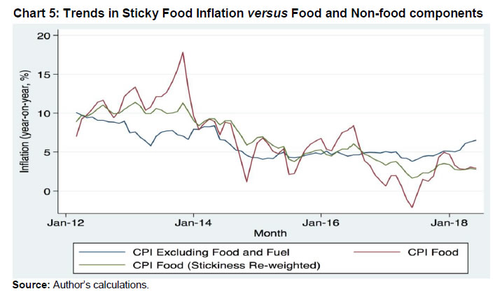 First, we obtain CPI data on food prices at the product group level. For each of the product groups, after multiplying the CPI weights with the duration estimates derived from reference prices, it is normalised to 100. Using these new weights, an aggregate stickiness weighted food price index is generated. We compare the trends in this measure with non-food component of CPI as well as the CPI food prices (official). The analysis was carried out on a monthly basis by estimating year-on-year inflation based on all the three measures and the period covers 2012-18. Overall, CPI inflation is much more volatile during the period as compared with the stickiness re-weighted food price inflation (Chart 5). Sticky food inflation and inflation excluding food and fuel do not coincide all the time. For example, the CPI excluding food and fuel inflation (conventional core inflation) declined during 2012-14 whereas the sticky food inflation remained almost constant. Similarly, since mid-2017, we see the inflation excluding food and fuel rising whereas the sticky food inflation remaining low. Given that food accounts for nearly half of the weight in CPI in India, this has significant implications for macroeconomic policy. For example, if the central bank uses ‘CPI excluding food and fuel’ as the only measure of inflation in a Taylor rule, under-prediction of inflation by the core on account of exclusion of sticky food prices can lead to lower than desired changes in interest rate and vice-versa. The bottom line is that macroeconomic models have to explicitly account for sticky component of food prices in this environment. VIII. Conclusion In this paper, we provide evidence of the extent of price stickiness in food sector in India using a newly constructed dataset for the period 2005-18. There is heterogeneity in the degree of price stickiness within food products and the duration of price spell goes up from 1.3 to 4.1 months if we use the reference prices (quarterly mode). Stylised facts about price-setting behaviour indicate that frequency of price change is synchronised across products and regions, co-move with inflation and exhibit strong seasonality in select products. Regression results show that both in posted as well as reference prices, frequency of price increases and decreases are significantly impacted by marginal cost shocks (proxied by the inflation at the product group level). At the aggregate level, both frequency and size of price change respond to marginal cost shocks in the case of reference prices. These empirical findings are in alignment with the predictions of a state-dependent pricing model with menu cost. The calibrated model shows that price-setting behaviour can be explained by differences in productivity process as well as menu costs. Finally, we show that trends in a stickiness re-weighted CPI food inflation do not perfectly align with CPI excluding food and fuel inflation, and therefore, the conventional measure of core inflation cannot fully capture the dynamics of sticky component of food price inflation. The findings of this study bring forth a number of issues which provide the scope for further research. As there are no aggregate level price stickiness estimates available for India, a natural extension of this study would be to compile data on non-food items and undertake a similar exercise. Also, given the finding of large heterogeneity across the country, spatial dimensions of price setting is another important dimension to which this study can be extended to. It would be interesting to study whether the law of one price holds across regions, how prices respond to shocks across regions with different characteristics in terms of economic development and institutions.
References Anand, R., Prasad, E. S., & Zhang, B. (2015). What measure of inflation should a developing country central bank target?. Journal of Monetary Economics, 74, 102-116. Aoki, K. (2001). Optimal monetary policy responses to relative-price changes. Journal of Monetary Economics, 48(1), 55-80. Banerji, A., & Meenakshi, J. V. (2004). Buyer collusion and efficiency of government intervention in wheat markets in northern India: An asymmetric structural auctions analysis. American Journal of Agricultural Economics, 86(1), 236-253. Banerjee, S. & R. Bhattacharya (2017), Micro-level price setting behaviour in India: evidence from group and sub-group level CPI-IW data, NIPFP Working paper No. 217 Berka, M., Devereux, M. B., & Rudolph, T. (2011). Price setting in a leading Swiss online supermarket (No. w17126). National Bureau of Economic Research. Bils, M., & Klenow, P. J. (2004). Some evidence on the importance of sticky prices. Journal of Political Economy, 112(5), 947985. Calvo, G. A. (1983). Staggered prices in a utility-maximizing framework. Journal of Monetary Economics, 12(3), 383-398. Catão, L. A., & Chang, R. (2015). World food prices and monetary policy. Journal of Monetary Economics, 75, 69-88. Cavallo, A. (2018). Scraped data and sticky prices. Review of Economics and Statistics, 100(1), 105-119. Chatterjee, Shoumitro (2017). Market Power and Spatial Competition in Rural India. Job Market Paper, Princeton University. Christiano, L. J., Eichenbaum, M., & Evans, C. L. (2005). Nominal rigidities and the dynamic effects of a shock to monetary policy. Journal of political Economy, 113(1), 1-45. Dhyne, E., Alvarez, L. J., Le Bihan, H., Veronese, G., Dias, D., Hoffmann, J. & Vilmunen, J. (2006). Price changes in the euro area and the United States: Some facts from individual consumer price data. Journal of Economic Perspectives, 20(2), 171-192. Dias, D. A., Marques, C. R., Neves, P. D., & Silva, J. S. (2005). On the Fisher–Konieczny index of price changes synchronization. Economics Letters, 87(2), 279-283. Dotsey, M., King, R. G., & Wolman, A. L. (1999). State-dependent pricing and the general equilibrium dynamics of money and output. The Quarterly Journal of Economics, 114(2), 655-690. Dube, A., Manning, A., & Naidu, S. (2018). Monopsony and Employer Mis-optimization Explain Why Wages Bunch at Round Numbers (No. w24991). National Bureau of Economic Research. Eichenbaum, M., Jaimovich, N., & Rebelo, S. (2011). Reference prices, costs, and nominal rigidities. American Economic Review, 101(1), 234-62. European Central Bank (2014). Base effects from the volatile components of the HICP and their impact on HICP inflation in 2014, Monthly Bulletin, ECB, February. Eusepi, S., Hobijn, B., & Tambalotti, A. (2011). CONDI: a cost-of-nominal-distortions index. American Economic Journal: Macroeconomics, 3(3), 53-91. Fisher, T. C., & Konieczny, J. D. (2000). Synchronization of price changes by multiproduct firms: evidence from Canadian newspaper prices. Economics Letters, 68(3), 271-277. Gagnon, E. (2009). Price setting during low and high inflation: Evidence from Mexico. The Quarterly Journal of Economics, 124(3), 1221-1263. Gertler, M., & Leahy, J. (2008). A Phillips curve with an Ss foundation. Journal of Political Economy, 116(3), 533-572. Golosov, M., & Lucas Jr, R. E. (2007). Menu costs and Phillips curves. Journal of Political Economy, 115(2), 171-199. Gouvea, S. (2007). Price rigidity in Brazil: Evidence from CPI micro data. Central Bank of Brazil Working Paper, 143. Head, A., Liu, L. Q., Menzio, G., & Wright, R. (2012). Sticky prices: A new monetarist approach. Journal of the European Economic Association, 10(5), 939-973. Kaplan, G., & Menzio, G. (2015). The morphology of price dispersion. International Economic Review, 56(4), 1165-1206. Kehoe, P. J., & Midrigan, V. (2008). Temporary price changes and the real effects of monetary policy (No. w14392). National Bureau of Economic Research. Klenow, P. J., & Kryvtsov, O. (2008). State-dependent or time-dependent pricing: Does it matter for recent US inflation?. The Quarterly Journal of Economics, 123(3), 863-904. Klenow, P. J., & Malin, B. A. (2010). Microeconomic evidence on price-setting. In Handbook of monetary economics (Vol. 3, pp. 231-284). Elsevier. Knotek, E. S. (2011). Convenient prices and price rigidity: cross-sectional evidence. Review of Economics and Statistics, 93(3), 1076-1086. Knotek, E. S. (2016). The Roles of Price Points and Menu Costs in Price Rigidity. 2016 Meeting Papers 1563. Society for Economic Dynamics. Levy, D., Lee, D., Chen, H., Kauffman, R. J., & Bergen, M. (2011). Price points and price rigidity. Review of Economics and Statistics, 93(4), 1417-1431. Mankiw, N. G., & Reis, R. (2003). What measure of inflation should a central bank target?. Journal of the European Economic Association, 1(5), 1058-1086. Midrigan, V. (2011). Menu costs, multiproduct firms, and aggregate fluctuations. Econometrica, 79(4), 1139-1180. Mishkin, F. S. (2008). Does stabilizing inflation contribute to stabilizing economic activity? (No. w13970). National Bureau of Economic Research. Nakamura, E., & Steinsson, J. (2008). Five facts about prices: A reevaluation of menu cost models. The Quarterly Journal of Economics, 123(4), 1415-1464. Nakamura, E., & Steinsson, J. (2010). Monetary non-neutrality in a multisector menu cost model. The Quarterly journal of economics, 125(3), 961-1013. Sheremirov, V. (2019). Price dispersion and inflation: New facts and theoretical implications. Journal of Monetary Economics. Silver, M. (2007). Core inflation: Measurement and statistical issues in choosing among alternative measures. IMF Staff Papers, 54(1), 163-190. Smets, F., & Wouters, R. (2007). Shocks and frictions in US business cycles: A Bayesian DSGE approach. American Economic Review, 97(3), 586-606. Tauchen, G. (1986). Finite state markov-chain approximations to univariate and vector autoregressions. Economics Letters, 20(2), 177-181. Taylor, J. B. (1980). Aggregate dynamics and staggered contracts. Journal of Political Economy, 88(1), 1-23.
Appendix | Appendix A: List of Items Covered and Weight in All India CPI-C | | Item | CPI Weight | Item | CPI Weight | | (1) | (2) | (1) | (2) | | Cereals and products | 8.51 | Milk and products | 6.90 | | Rice Common | 4.38 | Cowmilk | 6.42 | | Wheat(Desi) | 2.56 | Ghee | 0.47 | | Biscuit | 0.88 | Butter | 0.01 | | Jowar | 0.23 | Dairymilk | - | | Bajra | 0.11 | Oils and fats | 1.81 | | Bread | 0.11 | Mustard Oil | 1.33 | | Suji (Wheat) | 0.10 | Groundnutoil | 0.33 | | Maize | 0.06 | Coconut Oil | 0.08 | | Ragi | 0.05 | Vanaspati (Veg oil) | 0.07 | | Maida | 0.03 | Gingelioil | - | | Rice (Fine) | - | Fruits | 1.03 | | Rice (Superfine) | - | Banana | 0.56 | | Wheat (High Yeild) | - | Apple | 0.47 | | Atta (Wheat Flour) | - | Vegetables | 2.89 | | Pulses and products | 2.17 | Potato | 0.98 | | Arhar (Lentil) | 0.80 | Onion | 0.64 | | Moong (Pulses) | 0.35 | Tomato | 0.57 | | Masur (Lentil) | 0.30 | Brinjal | 0.37 | | Urad (Pulses) | 0.27 | Coriander | 0.33 | | Splitgram(Lentil) | 0.20 | Sugar & Confectionery | 1.23 | | Besan | 0.16 | Sugar | 1.13 | | Wholegram | 0.09 | Gur | 0.10 | | Meat and fish | 2.64 | Spices etc | 2.34 | | Fish(Rohu) | 1.27 | Tea | 0.96 | | Chicken | 1.23 | Redchilly | 0.58 | | Mutton | 0.14 | Turmeric | 0.50 | | Fish (Catfish) | - | Salt | 0.16 | | Fish(Pomphret) | - | Blackpepper | 0.14 | | Eggs | 0.43 | | | Note: ‘-’ indicates that the weight is combined with another item.
Source: Authors’ calculations and MOSPI. |
Appendix B: Robustness Check for Missing Data In this section, we look at the sensitivity of key results to the issue of missing observations. Out of the total of 691 weeks in the dataset, we do not have data on a continuous basis for all the centres. Discontinuities in reporting are caused by both missing observations as well as the data collection day being a holiday leading to no data collection in that week. Additionally, some of the centres were added to the dataset over the years while some other centres stopped reporting. This has made the data an unbalanced panel. Therefore, we check whether the discontinuities in data reporting drive our results. Since the primary interest of the study is to examine the frequency of price changes and not calculating inflation per se, availability of price data for any two consecutive weeks is sufficient to calculate a change observation. We have made the assumption that results are unaffected by the presence of missing observations and carried out the analysis incorporating all the change observations that can be generated from the data. We calculate key summary statistics on two restricted versions of sample and compare the results with that available from the full data set. In the first restricted sample, we drop those centres which did not report price observations for more than 25 per cent of the total number of weeks. This reduced the total number of centres to 61 as against 85 in our full sample. Further, we define a narrow set of centres, which recorded the most consistent reporting. First, we select those centres which have reported price observations for more than 75 per cent of the weeks. Among those centres, we further choose only those centres for which in each of the month, there were at least two change observations, which would require 3 continuous price points. Applying this criterion reduced the total number of centres to 17. In many centres, some of the products were not traded at all owing to different consumption pattern across the country. Therefore, applying this criterion uniformly across all the products was not possible. Hence, we select rice as the commodity on which the filter was applied as it is the most commonly reported item in our dataset. The reporting pattern suggests that once a centre reports price data for a week, it does report for all the commodities that are traded in that centre. Table B1 reports the frequency of price change as well as the average size of absolute change across all the major product groups. At the aggregate level, there is almost no change in the estimated frequency of price change across the filtered samples. If we look at the product level characteristics, we see that absolute size of change does not vary much across different sample sets (the maximum being variation of 0.02 in the case of vegetables). In change frequency, there are exceptions like vegetables and meat and fish, where the restricted sample frequency is higher by 5 percentage points. In terms of duration estimates, however, this translates to a lesser magnitude (0.47 to 0.40 months for vegetables and 0.99 to 0.74 months for meat and fish). Chart B1 reports the results at product level where we have plotted the change, increase and decrease frequencies as well as size of absolute change across different sample sets. Diagonal alignment of scatter plots indicates that even at product level the frequencies computed from different samples do not vary much. | Table B1: Change Frequency and Absolute Size of Change: Truncated versus Full Sample | | Product group | Change Frequency | Absolute Size of Change | | Full Sample | 61 centres* | 17 centres** | Full Sample | 61 centres* | 17 centres** | | (1) | (2) | (3) | (4) | (5) | (6) | (7) | | Milk and products | 0.04 | 0.04 | 0.04 | 0.09 | 0.08 | 0.1 | | Spices | 0.09 | 0.09 | 0.08 | 0.15 | 0.14 | 0.2 | | Cereals and products | 0.13 | 0.14 | 0.13 | 0.10 | 0.09 | 0.10 | | Oils and fats | 0.18 | 0.18 | 0.20 | 0.05 | 0.04 | 0.1 | | Meat and fish | 0.21 | 0.21 | 0.27 | 0.11 | 0.11 | 0.1 | | Egg | 0.21 | 0.21 | 0.24 | 0.10 | 0.09 | 0.1 | | Sugar and Confectionery | 0.23 | 0.23 | 0.24 | 0.05 | 0.04 | 0.1 | | Fruits | 0.25 | 0.25 | 0.26 | 0.16 | 0.14 | 0.2 | | Pulses and products | 0.28 | 0.29 | 0.33 | 0.06 | 0.05 | 0.1 | | Vegetables | 0.39 | 0.40 | 0.44 | 0.19 | 0.17 | 0.2 | | All Commodities (Mean) | 0.17 | 0.17 | 0.18 | 0.10 | 0.10 | 0.1 | | All Commodities (Median) | 0.16 | 0.16 | 0.16 | 0.09 | 0.08 | 0.1 | Note: * These centres reported data for more than 25% of the weeks in the sample.
** These centres reported data for more than 75% of the weeks and also had at most 2 missing change observations in every month (implying at least 3 continuous price observations).
Source: Authors’ calculations. | We also checked for the sensitivity of estimates of change frequency over time to missing data. Appendix D gives trends in the frequency of price change across major product groups over different sample sets as defined above. Overall, the trends observed in all the product groups are similar. Therefore, we can conclude that our results are largely robust to missing data, though estimates at individual product levels may contain some bias. 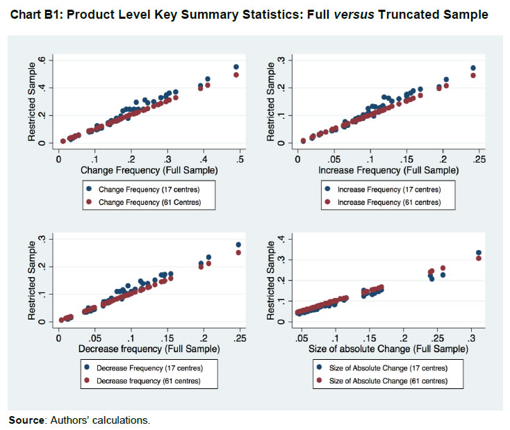
| Appendix C: Behaviour of Food Prices in India: Product level | | Product | Frequency of Price Change | Duration (Months) | Proportion of Price Increases | Average size of Price Change | Standard Deviation of Prices | Number of Observations | | (1) | (2) | (3) | (4) | (5) | (6) | (7) | | Tomato | 0.49 | 0.35 | 0.49 | 0.26 | 0.42 | 27549 | | Onion | 0.41 | 0.44 | 0.50 | 0.17 | 0.26 | 27803 | | Brinjal | 0.39 | 0.47 | 0.50 | 0.24 | 0.35 | 26219 | | Potato | 0.32 | 0.60 | 0.52 | 0.16 | 0.29 | 27771 | | Arhar | 0.31 | 0.64 | 0.52 | 0.05 | 0.11 | 27583 | | Moong | 0.30 | 0.66 | 0.52 | 0.05 | 0.12 | 27762 | | Urad | 0.30 | 0.66 | 0.51 | 0.06 | 0.16 | 27021 | | Splitgram | 0.28 | 0.70 | 0.53 | 0.06 | 0.14 | 26376 | | Apple | 0.27 | 0.73 | 0.54 | 0.15 | 0.34 | 24303 | | Wholegram | 0.26 | 0.76 | 0.53 | 0.07 | 0.19 | 25736 | | Masur | 0.25 | 0.82 | 0.53 | 0.05 | 0.14 | 24805 | | Chicken | 0.24 | 0.85 | 0.53 | 0.10 | 0.25 | 24478 | | Sugar | 0.23 | 0.87 | 0.51 | 0.05 | 0.08 | 27264 | | Banana | 0.22 | 0.94 | 0.52 | 0.16 | 0.34 | 26197 | | Fish3 | 0.22 | 0.96 | 0.55 | 0.12 | 0.57 | 9812 | | Eggs | 0.21 | 0.96 | 0.53 | 0.10 | 0.18 | 25156 | | Gur | 0.21 | 0.99 | 0.54 | 0.08 | 0.19 | 27079 | | Groundnut Oil | 0.21 | 1.00 | 0.56 | 0.04 | 0.20 | 22507 | | Mustard Oil | 0.21 | 1.01 | 0.55 | 0.05 | 0.15 | 25249 | | Fish1 | 0.20 | 1.07 | 0.55 | 0.14 | 0.59 | 6198 | | Besan | 0.19 | 1.09 | 0.55 | 0.07 | 0.16 | 24036 | | Jowar | 0.19 | 1.10 | 0.54 | 0.09 | 0.24 | 15876 | | Coconut Oil | 0.19 | 1.12 | 0.55 | 0.06 | 0.30 | 22193 | | Fish2 | 0.18 | 1.19 | 0.55 | 0.11 | 0.29 | 20887 | | Vanaspati | 0.17 | 1.24 | 0.56 | 0.05 | 0.14 | 23520 | | Continued next page |
| Appendix C: Behaviour of Food Prices in India: Product level (Concluded.) | | Product | Frequency of Price Change | Duration (Months) | Proportion of Price Increases | Average size of Price Change | Standard Deviation of Prices | Number of Observations | | (1) | (2) | (3) | (4) | (5) | (6) | (7) | | Black Pepper | 0.17 | 1.24 | 0.57 | 0.09 | 0.34 | 24690 | | Rice3 | 0.17 | 1.29 | 0.57 | 0.06 | 0.45 | 23029 | | Wheat2 | 0.16 | 1.34 | 0.57 | 0.08 | 0.27 | 22404 | | Rice2 | 0.16 | 1.34 | 0.57 | 0.06 | 0.29 | 25994 | | Gingelly Oil | 0.16 | 1.38 | 0.56 | 0.07 | 0.27 | 16732 | | Rice1 | 0.15 | 1.46 | 0.58 | 0.07 | 0.19 | 27671 | | Ragi | 0.15 | 1.48 | 0.57 | 0.08 | 0.27 | 10284 | | Bajra | 0.14 | 1.49 | 0.55 | 0.10 | 0.21 | 16561 | | Wheat1 | 0.14 | 1.52 | 0.56 | 0.07 | 0.30 | 12634 | | Maize | 0.14 | 1.57 | 0.55 | 0.10 | 0.29 | 20001 | | Atta | 0.12 | 1.84 | 0.58 | 0.07 | 0.21 | 25836 | | Maida | 0.11 | 1.93 | 0.58 | 0.08 | 0.15 | 25374 | | Suji | 0.11 | 2.04 | 0.59 | 0.08 | 0.18 | 25257 | | Mutton | 0.11 | 2.05 | 0.61 | 0.07 | 0.19 | 25570 | | Ghee | 0.10 | 2.11 | 0.62 | 0.06 | 0.21 | 24131 | | Red Chillies | 0.09 | 2.42 | 0.57 | 0.15 | 0.33 | 25221 | | Turmeric | 0.09 | 2.62 | 0.56 | 0.15 | 0.27 | 25557 | | Coriander | 0.08 | 2.64 | 0.57 | 0.16 | 0.32 | 24437 | | Butter | 0.06 | 4.07 | 0.70 | 0.11 | 0.19 | 22841 | | Milk (cow) | 0.05 | 4.90 | 0.69 | 0.09 | 0.16 | 25385 | | Milk (dairy) | 0.04 | 5.38 | 0.71 | 0.09 | 0.15 | 22817 | | Salt | 0.03 | 6.81 | 0.59 | 0.24 | 0.28 | 22635 | | Bread | 0.03 | 7.26 | 0.69 | 0.14 | 0.20 | 24433 | | Biscuit | 0.01 | 18.99 | 0.63 | 0.31 | 0.38 | 23912 | | All Products (Median) | 0.17 | 1.23 | 0.55 | 0.07 | 0.24 | | | All Products (Mean) | 0.17 | 1.29 | 0.58 | 0.10 | 0.24 | 1136786 | | Source: Authors’ calculations. |
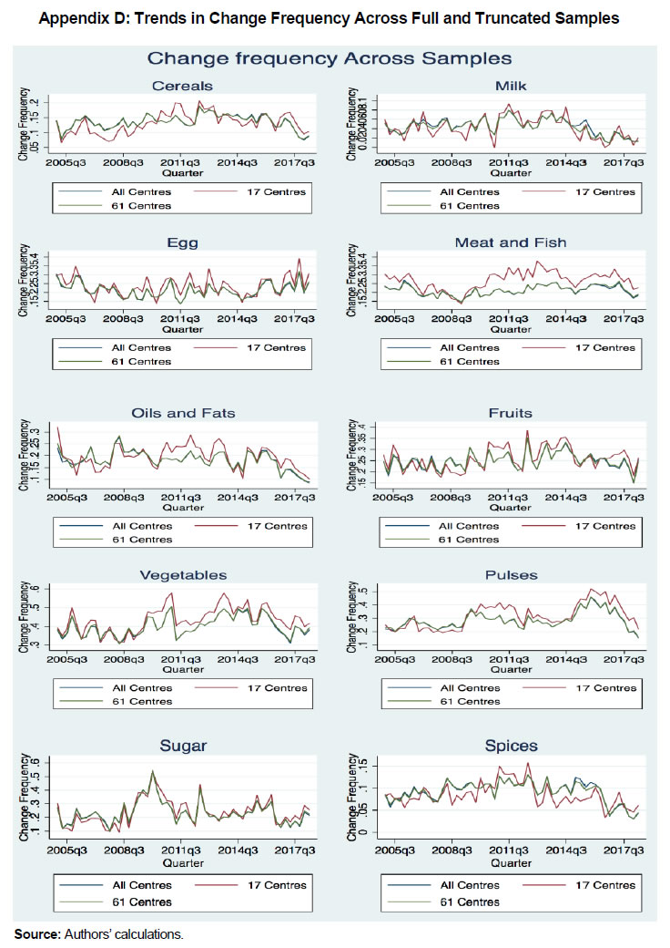
| Appendix E1: Estimates of Seasonal Effects on Frequency of Price Increase | | | Cereals | Meat & Fish | Egg | Milk | Oils & Fats | Fruits | Vege-tables | Pulses | Sugar | Spices | | (1) | (2) | (3) | (4) | (5) | (6) | (7) | (8) | (9) | (10) | (11) | | September | -0.01* | 0.00 | 0.01 | -0.01 | -0.01** | -0.02** | -0.03*** | -0.01 | -0.04*** | 0.00 | | | 0.00 | (0.01) | (0.01) | 0.00 | (0.01) | (0.01) | (0.01) | (0.01) | (0.01) | 0.00 | | October | -0.01** | 0.01 | 0.00 | 0.00 | -0.01 | 0.00 | 0.00 | 0.00 | -0.05*** | -0.01* | | | 0.00 | (0.01) | (0.01) | 0.00 | (0.01) | (0.01) | (0.01) | (0.01) | (0.01) | 0.00 | | November | 0.00 | 0.01 | 0.07*** | 0.00 | -0.01 | -0.01 | 0.00 | -0.01* | -0.05*** | -0.01 | | | 0.00 | (0.01) | (0.01) | 0.00 | (0.01) | (0.01) | (0.01) | (0.01) | (0.01) | 0.00 | | December | -0.01** | 0.02** | 0.07*** | 0.00 | -0.01 | -0.02** | -0.06*** | -0.04*** | -0.06*** | -0.01 | | | 0.00 | (0.01) | (0.01) | 0.00 | (0.01) | (0.01) | (0.01) | (0.01) | (0.01) | 0.00 | | January | -0.01* | 0.03*** | 0.04*** | 0.00 | 0.00 | 0.00 | -0.07*** | -0.05*** | -0.03*** | 0.00 | | | 0.00 | (0.01) | (0.01) | 0.00 | (0.01) | (0.01) | (0.01) | (0.01) | (0.01) | 0.00 | | February | -0.01** | 0.01 | 0.00 | 0.00 | -0.01** | 0.01 | -0.08*** | -0.04*** | -0.06*** | -0.01** | | | 0.00 | (0.01) | (0.01) | 0.00 | (0.01) | (0.01) | (0.01) | (0.01) | (0.01) | 0.00 | | March | -0.01*** | 0.02** | -0.03** | 0.00 | -0.01 | 0.03*** | -0.05*** | -0.04*** | -0.06*** | -0.02*** | | | 0.00 | (0.01) | (0.01) | 0.00 | (0.01) | (0.01) | (0.01) | (0.01) | (0.01) | 0.00 | | April | -0.01*** | 0.02* | -0.02 | 0.01 | 0.00 | 0.06*** | -0.02** | 0.01 | -0.03*** | 0.00 | | | 0.00 | (0.01) | (0.01) | 0.00 | (0.01) | (0.01) | (0.01) | (0.01) | (0.01) | 0.00 | | May | -0.01** | 0.03*** | 0.02 | 0.00 | 0.00 | 0.02** | 0.00 | 0.01 | -0.04*** | -0.01 | | | 0.00 | (0.01) | (0.01) | 0.00 | (0.01) | (0.01) | (0.01) | (0.01) | (0.01) | 0.00 | | June | -0.01** | 0.02*** | 0.04*** | 0.00 | -0.01 | 0.01 | 0.02** | -0.01 | -0.04*** | 0.00 | | | 0.00 | (0.01) | (0.01) | 0.00 | (0.01) | (0.01) | (0.01) | (0.01) | (0.01) | 0.00 | | July | 0.00 | 0.03*** | 0.03* | 0.00 | 0.00 | 0.01 | 0.05*** | 0.02*** | -0.01 | 0.00 | | | 0.00 | (0.01) | (0.01) | 0.00 | (0.01) | (0.01) | (0.01) | (0.01) | (0.01) | 0.00 | | N | 11246 | 3654 | 901 | 2653 | 5131 | 1831 | 3692 | 6423 | 1854 | 4442 | | adj. R2 | 0.140 | 0.232 | 0.392 | 0.179 | 0.233 | 0.283 | 0.275 | 0.348 | 0.219 | 0.248 | Note: *p<0.1, **p<0.05, ***p<0.01
Figures in parentheses are standard errors.
Source: Authors’ calculations. |
| Appendix E2: Estimates of Seasonal Effects on Frequency of Price Decrease | | | Cereals | Meat Fish | Egg | Milk | Oils Fats | Fruits | Vegetables | Pulses | Sugar | Spices | | (1) | (2) | (3) | (4) | (5) | (6) | (7) | (8) | (9) | (10) | (11) | | September | -0.01* | -0.01* | -0.02 | 0.00 | 0.01 | 0.02** | 0.04*** | 0.00 | 0.01 | 0.00 | | | 0.00 | (0.01) | (0.01) | 0.00 | (0.01) | (0.01) | (0.01) | (0.01) | (0.01) | 0.00 | | October | 0.00 | -0.02*** | -0.03** | 0.00 | 0.00 | -0.03*** | 0.03*** | -0.02*** | 0.01 | 0.00 | | | 0.00 | (0.01) | (0.01) | 0.00 | (0.01) | (0.01) | (0.01) | (0.01) | (0.01) | 0.00 | | November | 0.00 | -0.02*** | -0.06*** | 0.00 | 0.01* | -0.03*** | 0.03*** | 0.00 | 0.02* | 0.00 | | | 0.00 | (0.01) | (0.01) | 0.00 | (0.01) | (0.01) | (0.01) | (0.01) | (0.01) | 0.00 | | December | 0.00 | -0.01* | 0.00 | 0.00 | 0.00 | -0.06*** | 0.10*** | 0.02*** | 0.05*** | 0.00 | | | 0.00 | (0.01) | (0.01) | 0.00 | (0.01) | (0.01) | (0.01) | (0.01) | (0.01) | 0.00 | | January | 0.00 | -0.02*** | 0.01 | 0.01* | 0.00 | -0.06*** | 0.10*** | 0.03*** | 0.05*** | 0.00 | | | 0.00 | (0.01) | (0.01) | 0.00 | (0.01) | (0.01) | (0.01) | (0.01) | (0.01) | 0.00 | | February | 0.00 | -0.02** | 0.05*** | 0.00 | 0.02*** | -0.09*** | 0.07*** | 0.03*** | 0.05*** | 0.00 | | | 0.00 | (0.01) | (0.01) | 0.00 | (0.01) | (0.01) | (0.01) | (0.01) | (0.01) | 0.00 | | March | 0.01* | -0.02** | 0.06*** | 0.00 | 0.01** | -0.09*** | 0.03*** | 0.03*** | 0.04*** | 0.01 | | | 0.00 | (0.01) | (0.01) | 0.00 | (0.01) | (0.01) | (0.01) | (0.01) | (0.01) | 0.00 | | April | 0.00 | -0.01 | 0.05*** | 0.00 | 0.00 | -0.11*** | 0.00 | -0.01 | 0.01 | 0.00 | | | 0.00 | (0.01) | (0.01) | 0.00 | (0.01) | (0.01) | (0.01) | (0.01) | (0.01) | 0.00 | | May | 0.00 | -0.02*** | -0.01 | 0.00 | 0.00 | -0.10*** | -0.02** | 0.00 | 0.01 | 0.00 | | | 0.00 | (0.01) | (0.01) | 0.00 | (0.01) | (0.01) | (0.01) | (0.01) | (0.01) | 0.00 | | June | 0.00 | -0.02*** | -0.03** | 0.00 | 0.00 | -0.09*** | -0.04*** | -0.01 | 0.00 | 0.00 | | | 0.00 | (0.01) | (0.01) | 0.00 | (0.01) | (0.01) | (0.01) | (0.01) | (0.01) | 0.00 | | July | 0.00 | -0.02** | 0.00 | 0.00 | 0.01 | -0.06*** | -0.03*** | 0.00 | 0.00 | 0.00 | | | 0.00 | (0.01) | (0.01) | 0.00 | (0.01) | (0.01) | (0.01) | (0.01) | (0.01) | 0.00 | | N | 11246 | 3654 | 901 | 2653 | 5131 | 1831 | 3692 | 6423 | 1854 | 4442 | | adj. R2 | 0.155 | 0.215 | 0.479 | 0.204 | 0.181 | 0.310 | 0.279 | 0.311 | 0.243 | 0.261 | Note: *p<0.1, **p<0.05, ***p<0.01.
Figures in parenthesis are standard errors.
Source: Authors’ calculations. |
| Appendix F1: FK Measure of Synchronisation and χ2 test values: Products | | No. | Product | FK measure | Dias Q | No. | Product | FK measure | Dias Q | | (1) | (2) | (3) | (4) | (1) | (2) | (3) | (4) | | 1 | Apple | 0.22 | 1168.0 | 26 | Mutton | 0.19 | 889.5 | | 2 | Arhar | 0.26 | 1874.9 | 27 | Onion | 0.29 | 2366.5 | | 3 | Atta | 0.19 | 937.8 | 28 | Potato | 0.23 | 1448.4 | | 4 | Bajra | 0.22 | 801.8 | 29 | Ragi | 0.28 | 839.4 | | 5 | Banana | 0.19 | 907.9 | 30 | Red Chillies | 0.18 | 861.7 | | 6 | Besan | 0.23 | 1306.8 | 31 | Rice1 | 0.17 | 840.6 | | 7 | Biscuit | 0.18 | 770.0 | 32 | Rice2 | 0.18 | 832.8 | | 8 | Bread | 0.18 | 798.5 | 33 | Rice3 | 0.19 | 798.1 | | 9 | Brinjal | 0.17 | 785.2 | 34 | Sugar | 0.30 | 2422.4 | | 10 | Butter | 0.20 | 915.9 | 35 | Suji | 0.19 | 914.3 | | 11 | Chicken | 0.19 | 883.9 | 36 | Tomato | 0.21 | 1267.4 | | 12 | Eggs | 0.20 | 1039.4 | 37 | Turmeric | 0.20 | 979.9 | | 13 | Fish1 | 0.34 | 763.3 | 38 | Urad | 0.23 | 1409.1 | | 14 | Fish2 | 0.18 | 709.9 | 39 | Vanaspati | 0.21 | 1028.2 | | 15 | Fish3 | 0.26 | 712.8 | 40 | Black Pepper | 0.19 | 916.2 | | 16 | Ghee | 0.19 | 903.7 | 41 | Coconut oil | 0.20 | 868.4 | | 17 | Gingelly Oil | 0.21 | 766.4 | 42 | coriander | 0.19 | 848.7 | | 18 | Groundnut Oil | 0.19 | 845.4 | 43 | Milk(cow) | 0.19 | 895.0 | | 19 | Gur | 0.20 | 1095.3 | 44 | Milk (dairy) | 0.20 | 899.4 | | 20 | Jowar | 0.21 | 719.4 | 45 | salt | 0.19 | 828.7 | | 21 | Maida | 0.19 | 945.7 | 46 | Split gram | 0.25 | 1627.5 | | 22 | Maize | 0.20 | 799.3 | 47 | wheat1 | 0.26 | 837.6 | | 23 | Masur | 0.23 | 1273.5 | 48 | wheat2 | 0.21 | 974.6 | | 24 | Moong | 0.22 | 1331.1 | 49 | Whole gram | 0.24 | 1519.8 | | 25 | Mustard Oil | 0.21 | 1179.2 | | | | | Note: All the Q values are significant at 1 per cent with degrees of freedom (T-1)
Source: Authors’ calculations. |
| Appendix F2: FK Measure of Synchronisation and χ2 test values: Centres | | No. | Centre | FK Measure | Dias Q | No. | Centre | FK Measure | Dias Q | | (1) | (2) | (3) | (4) | (1) | (2) | (3) | (4) | | 1 | Agartala | 0.55 | 5496.41 | 32 | Jaipur | 0.49 | 5351.71 | | 2 | Agra | 0.51 | 3403.22 | 33 | Jalpaiguri | 0.59 | 3179.94 | | 3 | Aizwal | 0.50 | 5271.45 | 34 | Jammu | 0.51 | 5295.40 | | 4 | Allahabad | 0.65 | 7290.76 | 35 | Jodhpur | 0.53 | 5825.43 | | 5 | Amritsar | 0.62 | 3677.25 | 36 | Kanpur | 0.70 | 6271.41 | | 6 | Asansol | 0.56 | 4248.52 | 37 | Karnal | 0.49 | 3122.72 | | 7 | Bangalore | 0.45 | 3492.08 | 38 | Khozhikode | 0.40 | 4349.77 | | 8 | Bhatinda | 0.41 | 2044.48 | 39 | Kohima | 0.80 | 4403.63 | | 9 | Bhopal | 0.36 | 3583.18 | 40 | Kolkata | 0.45 | 4407.67 | | 10 | Bhubneshwar | 0.36 | 3395.10 | 41 | Kurnool | 0.49 | 5503.41 | | 11 | Bijapur | 0.44 | 2326.02 | 42 | Lucknow | 0.28 | 2125.66 | | 12 | Chennai | 0.46 | 4827.93 | 43 | Ludhiana | 0.63 | 6077.16 | | 13 | Chittoor | 0.53 | 6965.60 | 44 | Madurai | 0.65 | 4837.03 | | 14 | Coimbatore | 0.54 | 6332.34 | 45 | Malda | 0.53 | 2408.83 | | 15 | Cuttack | 0.50 | 3124.39 | 46 | Mandi | 0.56 | 4785.05 | | 16 | Dausa | 0.48 | 5968.96 | 47 | Mumbai | 0.42 | 4238.45 | | 17 | Delhi | 0.37 | 3251.15 | 48 | Nagpur | 0.43 | 1769.79 | | 18 | Dhanbad | 0.47 | 2965.35 | 49 | Nasik | 0.64 | 2608.93 | | 19 | Dibrugarh | 0.51 | 4393.83 | 50 | Panaji | 0.61 | 7000.53 | | 20 | Dispur | 0.46 | 2035.74 | 51 | Patna | 0.37 | 3771.44 | | 21 | Ernakulam | 0.44 | 4643.01 | 52 | Port blair | 0.56 | 8478.81 | | 22 | Gandhi Nagar | 0.42 | 3475.31 | 53 | Ranchi | 0.47 | 5155.47 | | 23 | Gorakhpur | 0.61 | 7715.09 | 54 | Saharanpur | 0.58 | 4066.30 | | 24 | Guntur | 0.48 | 4445.10 | 55 | Salem | 0.59 | 5080.08 | | 25 | Guwahati | 0.50 | 4320.10 | 56 | Shillong | 0.48 | 5588.44 | | 26 | Hissar | 0.53 | 5314.78 | 57 | Swaimadhopur | 0.42 | 3009.32 | | 27 | Howrah | 0.47 | 2472.18 | 58 | Tirunelveli | 0.50 | 2294.75 | | 28 | Hubli | 0.60 | 5333.11 | 59 | Trivandrum | 0.45 | 4822.79 | | 29 | Hyderabad | 0.45 | 5196.90 | 60 | Tumkur | 0.55 | 4918.13 | | 30 | Imphal | 0.40 | 2479.23 | 61 | Udaipur | 0.49 | 3382.31 | | 31 | Itanagar | 0.52 | 2404.71 | 62 | Vishakhapatnam | 0.47 | 5603.51 | Note: All the Q values are significant at 1 per cent with degrees of freedom (T-1)
Source: Authors’ calculations. |
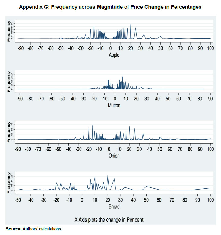 |