States continued to post surplus in the revenue account in 2012-13 as in recently preceding years, largely driven by own revenues. In 2013-14(RE), however, the revenue surplus was nearly wiped away and the fiscal deficit at the consolidated level just met the target set by the Thirteenth Finance Commission. Most states reaffirmed their commitment to fiscal consolidation in 2014-15, although some budgeted for higher deficits than stipulated under their FRBM Acts. Freeing up resources for higher capital outlays, improving the quality of fiscal consolidation and setting the consolidated debt-GDP ratio of the states on a declining trajectory are crucial for improving the health of state finances. 1. Introduction 3.1 In the post-global crisis period, all states have amended their fiscal responsibility legislations in 2010-11 in order to recommit to rule-based fiscal consolidation. Although the progress in this direction continued up to 2011-12, some deterioration has been observed during 2012-14. The key deficit indicators were, however, budgeted to improve in 2014-15. 2. Accounts: 2012-13 3.2 Key deficit indicators of the states at the consolidated level marginally deteriorated in 2012-13, but they were well within the Thirteenth Finance Commission’s (FC-XIII) targets (Table III.1). Although both non-special category (NSC) states and special category (SC) states continued to post revenue surpluses, the latter outperformed their non-SC peers, recording lower deficits than a year ago (Table III.2). 3.3 Revenue receipts grew largely on account of states’ own tax collections, particularly sales tax/value added tax (VAT) which led to a marginal improvement in states’ own tax revenue-GDP ratio. Transfers from the centre, on the other hand, expanded at a slower pace, mainly on account of the sharp deceleration in the growth of grants from the centre which, as a proportion to GDP, declined over the previous year (Table III.3). Non-debt capital receipts registered a steep decline over the previous year, primarily on account of a decline in recovery of loans. | Table III.1: Major Deficit Indicators of State Governments | | (Amount in ₹ billion) | | Item | 2011-12 | 2012-13 | 2013-14 (BE) | 2013-14 (RE) | 2014-15 (BE) | | 1 | 2 | 3 | 4 | 5 | 6 | | Revenue Deficit | -239.6 | -203.2 | -477.3 | -29.5 | -541.7 | | (-0.3) | (-0.2) | (-0.4) | (-0.0) | (-0.4) | | Gross Fiscal Deficit | 1,683.5 | 1,954.7 | 2,450.5 | 2,835.0 | 2,950.6 | | (1.9) | (2.0) | (2.2) | (2.5) | (2.3) | | Primary Deficit | 315.4 | 450.0 | 716.7 | 1,113.7 | 1,018.6 | | (0.4) | (0.5) | (0.6) | (1.0) | (0.8) | BE: Budget Estimates. RE: Revised Estimates.
Note: 1. Negative (-) sign indicates surplus.
2. Figures in parentheses are per centages to GDP.
3. The ratios to GDP at current market prices are based on new GDP series (Base:2011-12) released by CSO in early 2015.
Source: Budget documents of state governments. |
| Table III.2: Fiscal Imbalances in Non-Special and Special Category States | | (Per cent to GSDP) | | | 2011-12 | 2012-13 | 2013-14 (RE) | 2014-15 (BE) | | 1 | 2 | 3 | 4 | 5 | | Revenue Deficit | | | | | | Non-Special Category States | -0.2 | -0.1 | 0.1 | -0.3 | | Special Category States | -2.0 | -2.0 | -1.7 | -2.8 | | All States Consolidated* | -0.3 | -0.2 | 0.0 | -0.4 | | Gross Fiscal Deficit | | | | | | Non-Special Category States | 2.2 | 2.3 | 2.8 | 2.6 | | Special Category States | 2.8 | 2.4 | 4.9 | 3.1 | | All States Consolidated* | 1.9 | 2.0 | 2.5 | 2.3 | | Primary Deficit | | | | | | Non-Special Category States | 0.4 | 0.6 | 1.1 | 0.9 | | Special Category States | 0.4 | 0.0 | 2.5 | 0.9 | | All States Consolidated* | 0.4 | 0.5 | 1.0 | 0.8 | | Primary Revenue Deficit | | | | | | Non-Special Category States | -2.0 | -1.8 | -1.7 | -2.1 | | Special Category States | -4.4 | -4.4 | -4.0 | -5.0 | | All States Consolidated* | -1.8 | -1.7 | -1.5 | -1.9 | * : As a ratio to GDP. BE: Budget Estimates. RE: Revised Estimates.
Note: Negative (-) sign indicates surplus.
Source: Budget documents of state governments. | 3.4 Revenue expenditure decelerated in 2012- 13 (Table III.4). The deceleration was more pronounced in the non-development component, particularly pensions and administrative services, despite an increase in interest payments (IP) at a faster pace than a year ago. While the growth in development revenue expenditure was broadly maintained, this was on account of the sharp increase in subsidies to state power utilities and expenditure on rural development offsetting the deceleration in other major social and economic services. The slowdown in receipt under plan grants from the centre could have affected associated expenditures by the states. Capital outlay for the transport sector expanded strongly on account of roads and bridges, reflecting the thrust on infrastructure development. However, capital outlays on energy contracted in 2012-13, reflecting the fragile condition of the power sector (Table III.4). Of particular concern is the continuing shrinkage of investment in the energy sector at a time when power shortages have been tightening into a binding constraint on growth. This, in turn, reflects the deepening malaise in the power utilities at the state level (Box III.1). Consequently, overall capital outlay as a proportion to GDP recorded virtually no improvement in 2012-13 (Table III.5). These developments suggest that although states made efforts to strengthen their resolve on fiscal prudence by pushing up their own tax effort, the quality of expenditure was constrained by outgoes under subsidies and committed expenditures. | Table III.3: Aggregate Receipts of State Governments | | (Amount in ₹ billion) | | Item | 2011-12 | 2012-13 | 2013-14 (RE) | 2014-15 (BE) | | 1 | 2 | 3 | 4 | 5 | | Aggregate Receipts (1+2) | 12,943.4 | 14,508.6 | 17,663.7 | 20,892.4 | | (14.7) | (14.5) | (15.6) | (16.2) | | 1. Revenue Receipts (a+b) | 10,985.3 | 12,520.2 | 14,986.2 | 18,566.6 | | (12.4) | (12.5) | (13.2) | (14.4) | | a. States' Own Revenue (i+ii) | 6,565.2 | 7,718.1 | 8,866.5 | 9,957.9 | | (7.4) | (7.7) | (7.8) | (7.7) | | i. States' Own Tax | 5,574.0 | 6,545.5 | 7,528.6 | 8,398.7 | | (6.3) | (6.6) | (6.6) | (6.5) | | ii. States' Own Non-Tax | 991.3 | 1,172.6 | 1,337.9 | 1,559.2 | | (1.1) | (1.2) | (1.2) | (1.2) | | b. Current Transfers (i+ii) | 4,420.1 | 4,802.1 | 6,119.7 | 8,608.7 | | (5.0) | (4.8) | (5.4) | (6.7) | | i. Shareable Taxes | 2,555.9 | 2,915.3 | 3,319.9 | 3,857.6 | | (2.9) | (2.9) | (2.9) | (3.0) | | ii. Grants-in Aid | 1,864.2 | 1,886.8 | 2,799.7 | 4,751.1 | | (2.1) | (1.9) | (2.5) | (3.7) | | 2. Capital Receipts (a+b) | 1,958.1 | 1,988.4 | 2,677.6 | 2,325.9 | | (2.2) | (2.0) | (2.4) | (1.8) | | a. Non-Debt Capital Receipts | 178.2 | 73.7 | 94.2 | 74.6 | | (0.2) | (0.1) | (0.1) | (0.1) | | i. Recovery of Loans and Advances | 171.6 | 72.6 | 89.6 | 61.2 | | (0.2) | (0.1) | (0.1) | (0.0) | | ii. Miscellaneous Capital Receipts | 6.7 | 1.0 | 4.6 | 13.3 | | (0.0) | (0.0) | (0.0) | (0.0) | | b. Debt Receipts | 1,779.8 | 1,914.7 | 2,583.4 | 2,251.3 | | (2.0) | (1.9) | (2.3) | (1.7) | | i. Market Borrowings | 1,354.0 | 1,462.5 | 2,006.4 | 2,293.0 | | (1.5) | (1.5) | (1.8) | (1.8) | | ii. Other Debt Receipts | 425.9 | 452.2 | 576.9 | -41.7 | | (0.5) | (0.5) | (0.5) | (0.0) | BE: Budget Estimates RE: Revised Estimates.
Note: 1. Figures in parentheses are per centages to GDP.
2. Debt Receipts are on net basis.
Source: Budget documents of state governments. |
| Table III.4: Variation in Major Items | | (Amount in ₹ billion) | | Item | 2011-12 | 2012-13 | 2013-14 | 2014-15 | | Accounts | Per cent Varition Over 2010-11 | Accounts | Per cent Variation Over 2011-12 | RE | Per cent Variation Over 2012-13 | BE | Per cent Variation Over 2013-14 (RE) | | 1 | 2 | 3 | 4 | 5 | 6 | 7 | 8 | 9 | | I. Revenue Receipts (i+ii) | 10985.3 | 17.4 | 12,520.2 | 14.0 | 14,986.2 | 19.7 | 18,566.6 | 23.9 | | (i) Tax Revenue (a+b) | 8129.9 | 19.5 | 9,460.8 | 16.4 | 10,848.5 | 14.7 | 12,256.3 | 13.0 | | (a) Own Tax Revenue | 5574.0 | 21.0 | 6,545.5 | 17.4 | 7,528.6 | 15.0 | 8,398.7 | 11.6 | | of which: Sales Tax | 3450.6 | 23.7 | 4,038.5 | 17.0 | 4,815.3 | 19.2 | 5,367.9 | 11.5 | | (b) Share in Central Taxes | 2555.9 | 16.4 | 2,915.3 | 14.1 | 3,319.9 | 13.9 | 3,857.6 | 16.2 | | (ii) Non-Tax Revenue | 2855.4 | 11.9 | 3,059.4 | 7.1 | 4,137.7 | 35.2 | 6,310.3 | 52.5 | | (a) States' Own Non-Tax Revenue | 991.3 | 8.2 | 1,172.6 | 18.3 | 1,337.9 | 14.1 | 1,559.2 | 16.5 | | (b) Grants from Centre | 1864.2 | 14.0 | 1,886.8 | 1.2 | 2,799.7 | 48.4 | 4,751.1 | 69.7 | | II. Revenue Expenditure | 10745.7 | 15.3 | 12,317.0 | 14.6 | 14,956.6 | 21.4 | 18,024.9 | 20.5 | | of which: | | | | | | | | | | (i) Development Expenditure | 6505.9 | 16.9 | 7,584.1 | 16.6 | 9,399.3 | 23.9 | 11,638.0 | 23.8 | | of which: Education, Sports, Art and Culture | 2160.7 | 15.2 | 2,454.0 | 13.6 | 2,947.7 | 20.1 | 3,551.0 | 20.5 | | Transport and Communication | 273.6 | 24.4 | 319.1 | 16.6 | 373.2 | 17.0 | 413.0 | 10.7 | | Power | 460.1 | 25.7 | 629.4 | 36.8 | 656.4 | 4.3 | 776.6 | 18.3 | | Relief on account of Natural Calamities | 136.9 | 56.3 | 109.8 | -19.8 | 179.1 | 63.1 | 134.8 | -24.7 | | Rural Development | 372.2 | 14.2 | 443.7 | 19.2 | 585.3 | 31.9 | 1,178.9 | 101.4 | | (ii) Non-Development Expenditure | 3927.4 | 12.1 | 4,375.7 | 11.4 | 5,073.3 | 15.9 | 5,856.9 | 15.4 | | of which: Administrative Services | 859.8 | 14.4 | 960.9 | 11.8 | 1,167.3 | 21.5 | 1,380.0 | 18.2 | | Pension | 1278.0 | 18.1 | 1,447.5 | 13.3 | 1,638.5 | 13.2 | 1,868.7 | 14.1 | | Interest Payments | 1368.2 | 9.6 | 1,504.7 | 10.0 | 1,721.3 | 14.4 | 1,932.0 | 12.2 | | III. Net Capital Receipts # | 1958.1 | 17.0 | 1,988.4 | 1.5 | 2,677.6 | 34.7 | 2,325.9 | -13.1 | | of which: Non-Debt Capital Receipts | 178.2 | -46.4 | 74.1 | -58.4 | 94.2 | 27.0 | 74.6 | -20.8 | | IV. Capital Expenditure $ | 2101.4 | 23.1 | 2,231.6 | 6.2 | 2,958.7 | 32.6 | 3,566.8 | 20.6 | | of which: Capital Outlay | 1712.5 | 12.7 | 1,931.8 | 12.8 | 2,652.7 | 37.3 | 3,362.8 | 26.8 | | of which: Capital Outlay on Irrigation and Flood Control | 467.3 | 8.0 | 497.0 | 6.4 | 630.9 | 26.9 | 643.7 | 2.0 | | Capital Outlay on Energy | 195.5 | 22.9 | 185.0 | -5.4 | 214.4 | 15.9 | 316.0 | 47.4 | | Capital Outlay on Transport | 378.2 | 8.5 | 452.9 | 19.7 | 577.7 | 27.6 | 679.4 | 17.6 | | Memo Item: | | | | | | | | | | Revenue Deficit | -239.6 | 685.6 | -203.2 | -15.2 | -29.5 | -85.5 | -541.7 | 1733.1 | | Gross Fiscal Deficit | 1683.5 | 4.3 | 1,954.7 | 16.1 | 2,835.0 | 45.0 | 2,950.6 | 4.1 | | Primary Deficit | 315.4 | -13.9 | 450.0 | 42.7 | 1,113.7 | 147.5 | 1,018.6 | -8.5 | BE: Budget Estimates RE: Revised Estimates.
# : It includes the following items on net basis: internal debt; loans and advances from the centre; inter-state settlement; contingency fund; small savings, provident funds etc.; reserve funds; deposits and advances; suspense and miscellaneous; appropriation to contingency fund and remittances.
$ : Capital Expenditure includes Capital Outlay and Loans and Advances by State Governments.
Note: 1. Negative (-) sign in deficit indicators indicates surplus.
2. Also see Notes to Appendices.
Source: Budget documents of state governments. | Box III.1: State Power Utilities and State Finances Power sector reforms were initiated in the early nineties, with enactment of the Electricity Laws (Amendment) Act, 1991 to encourage the entry of privately owned power generation companies and introduction of the mega power policy (MPP) in 1995 to leverage the development of large size power projects and derive benefit from economies of scale. The central government enacted the Electricity Regulatory Commission (ERC) Act, 1998 and introduced a provision for states to create their own State Electricity Regulation Commissions (SERCs). The Electricity Act, 2003 which consolidated the laws relating to generation, transmission, distribution, trading and use of electricity, sought to create a liberal framework for the development of the power sector by distancing government from regulation. Despite the aforementioned reforms, the financial performance of state power utilities (SPUs), particularly those engaged in distribution, has deteriorated considerably over the years, mainly on account of inadequate tariffs, high transmission and distribution (T&D) losses, absence of full metering and inefficiencies in billing and collection. Mounting losses of the power distribution companies (discoms) are financed through short-term borrowings from banks and other financial institutions (FIs) or through diversion of longterm loans to cover such losses. Impact of Financials of Power Utilities on State Finances With the state governments owning most of the power discoms, deterioration in the financial health of these entities invariably affects the fiscal position of the states. The state governments extend financial support to SPUs through various means such as providing subsidies and grants as compensation for power given to certain groups, make equity investments in state power discoms, provide direct loans and extend guarantees for the loans obtained from banks/financial institutions. Though these guarantees are in the nature of contingent liabilities, any credit default by SPUs would entail that state governments bear the burden. In the past, the state governments had issued power bonds under the one-time settlement scheme in 2003-04 to clear the dues of SEBs to central PSUs which added to their interest and repayment burden. Impact of Financial Restructuring Plan (FRP)1 The FRP for state power discoms would impact the finances of the eight states2 participating in it. On the receipts side, the conversion of loans into equity or adjustment of electricity duty and other statutory charges against subsidy support would imply lower receipts. On the expenditure side, there would be additional expenditure due to (i) interest burden in respect of 50 per cent of the short-term liabilities (STL) issued as bonds by the discoms and subsequently taken over by state governments as special securities; (ii) repayment of the special securities (after the moratorium period of 3-5 years); (iii) support to the discoms in respect of their cash losses during 2012-13 and in the subsequent period depending on the sharing arrangements between banks/financial institutions and state governments; (iv) equity/loan support towards capital expenditure to be incurred by distribution companies for additional distribution network and strengthening of the existing system; and (v) additional support to the distribution companies in the form of equity or interest free loan in case of any shortfall in adhering to the annual performance projections under the FRP. Apart from the impact on the finances of states, restructured loans to the power discoms also adds to the debt and contingent liabilities of the participating states. Way Forward Going by the magnitude of the implications for state finances, it is important that state governments do not make debt restructuring a perpetual feature, considering the downside risks to stability of state finances. Viability of discoms is more critical in states that provide free or heavily subsidised power supply to the agriculture sector or have not revised tariffs periodically. Regular tariff revisions in line with cost escalation, improvement in operational efficiency including reduction in aggregate technical and commercial (AT&C) losses and collection of revenue arrears may also help to reduce the gap between average cost of supply (ACS) and average revenue realized (ARR). Apart from time-bound full metering for all consumers, FC-XIV has also recommended amendment of the Electricity Act, 2003 with provision of penalties on state governments for delays in the payment of subsidies. Further, it has also recommended the constitution of a SERC Fund by all states to provide financial autonomy to the SERCs. Improvement in efficiency and viability of the state discoms is crucial for reducing the pressure on state finances in the medium-term while also providing some relief to lenders, particularly banks/financial institutions, keeping in view financial stability considerations. | Table III.5: Expenditure Pattern of State Governments | | (Amount in ₹ billion) | | Item | 2011-12 | 2012-13 | 2013-14 (RE) | 2014-15 (BE) | | 1 | 2 | 3 | 4 | 5 | | Aggregate Expenditure (1+2 = 3+4+5) | 12,847.1 | 14,548.6 | 17,915.3 | 21,591.7 | | (14.5) | (14.6) | (15.8) | (16.8) | | 1. Revenue Expenditure of which: | 10,745.7 | 12,317.0 | 14,956.6 | 18,024.9 | | (12.2) | (12.3) | (13.2) | (14.0) | | Interest payments | 1,368.2 | 1,504.7 | 1,721.3 | 1,932.0 | | (1.5) | (1.5) | (1.5) | (1.5) | | 2. Capital Expenditure of which: | 2,101.4 | 2,231.6 | 2,958.7 | 3,566.8 | | (2.4) | (2.2) | (2.6) | (2.8) | | Capital outlay | 1,712.5 | 1,931.8 | 2,652.7 | 3,362.8 | | (1.9) | (1.9) | (2.3) | (2.6) | | 3. Development Expenditure | 8,524.1 | 9,722.6 | 12,145.0 | 14,942.5 | | (9.7) | (9.7) | (10.7) | (11.6) | | 4. Non-Development Expenditure | 4,010.6 | 4,468.8 | 5,286.3 | 6,119.2 | | (4.5) | (4.5) | (4.7) | (4.8) | | 5. Others* | 312.4 | 357.2 | 484.0 | 530.0 | | (0.4) | (0.4) | (0.4) | (0.4) | RE: Revised Estimates BE: Budget Estimates.
*: Includes grants-in-aid and contributions (compensation and assignments to local bodies).
Note: 1. Figures in parentheses are per cent to GDP.
2. Capital Expenditure includes Capital Outlay and Loans and Advances by State Governments.
Source: Budget documents of state governments. | 3. Revised Estimates: 2013-14 3.5 The fiscal position of state governments deteriorated in 2013-14 as revealed in the revised estimates for that year (Table III.1), both in relation to budget forecasts as well as from the position a year ago. The revenue accounts of 18 states deteriorated over the previous year, with diminished surplus in nine states, reversal from surplus to balance/deficit in six states and increase in deficit in three states. For all states taken together, the modest revenue surplus recorded in the preceding year was wiped away to near-balance. Underlying this erosion was a slowdown in both own tax and non-tax revenues. Notwithstanding an improvement in the state VAT revenue growth, other major own tax revenues were affected by the sluggishness in the economy. Factors such as lacklustre real estate market, slow down in automobile sales and a financially weak power sector affected collections under land revenue, stamp duties, taxes on vehicles, and duties on electricity. In fact, the deterioration in states’ revenue accounts would have been even more deleterious but for the cushion provided by grants from the centre, which recorded a robust growth of 48.4 per cent in 2013-14 (RE) over the previous year, reflecting the base effect3. 3.6 At the same time, growth in revenue expenditure increased significantly over the previous year on account of increase in social sector expenditure and certain economic services such as soil and water conservation and food storage and warehousing. Although growth in nondevelopment revenue expenditure increased over the previous year, particularly under administrative services and interest payments, it was lower than the budget estimates for the year. 3.7 The GFD as a proportion to GSDP widened at the consolidated level, reflecting the sizeable shrinkage of the revenue surplus, as also higher capital outlay in transport, irrigation and flood control and energy (Table III.4 and III.6). The capital outlay on food and warehousing declined, despite there being a need for higher allocations in preparation for the implementation of the National Food Security Act, 2012. While the overall GFD-GDP ratio at 2.5 per cent was in line with FC-XIII target, state-wise position shows that 12 out of the 28 states – 6 of which were in the non-special category – could not meet the FCXIII’s target. 4. Budget Estimates: 2014-15 Key Deficit Indicators 3.8 The experience with deteriorating fiscal accounts, particularly in 2013-14, evidently weighed upon state governments. Budget estimates for 2014-15 reaffirmed the intent of states to recommit to fiscal consolidation (Table III.1). The consolidated revenue surplus of the states was budgeted to expand sizeably on account of a higher growth in revenue receipts visa- vis revenue expenditure (Table III.3). As many as 17 states intended to improve their revenue surpluses and 15 states, their GFD-GSDP ratios (Table III.6). As indicated in Chapter I, however, six out of the 29 states (including bifurcated Andhra Pradesh) budgeted for revenue deficits during 2014-15 and 10 states budgeted for GFD-GSDP ratios higher than 3 per cent, thereby diluting the recommendation of FC-XIII. Revenue Receipts 3.9 Revenue receipts are budgeted to increase significantly, with the entire increase emanating from higher grants from the centre in view of the change in the accounting of financial assistance for the centrally sponsored schemes (CSS) (Box III.2, Tables III.3 and III.4). By contrast, states’ own revenue-GDP ratio is expected to show a marginal decline on account of deceleration in all major taxes. Thus, the projected improvement in revenue balances has little to do with states’ own efforts. Expenditure Pattern 3.10 Growth in revenue expenditure was budgeted to increase under crop husbandry, rural development, education and health, partly reflecting higher plan outlays under those centrally sponsored schemes which are now being routed through the state budgets. Revenue expenditure growth in industries and energy was expected to increase significantly, mainly on account of expenditure on subsidies. Non-development expenditure growth, on the other hand, was to marginally decelerate, mainly on account of a deceleration in the growth of committed expenditure other than pension. Growth in grants to local bodies was to decelerate sharply, resulting in a reduction in its share in revenue expenditure to 2.9 per cent as against 3.2 per cent in 2013-14 (RE). The reduced devolution of resources to the lower tiers of government may not augur well for fiscal decentralisation. | Table III.6: Deficit Indicators of State Governments | | (Per cent) | | State | 2012-13 | 2013-14 (RE) | 2014-15 (BE) | | RD/ GSDP | GFD/ GSDP | PD/ GSDP | PRD/ GSDP | RD/ GSDP | GFD/ GSDP | PD/ GSDP | PRD/ GSDP | RD/ GSDP | GFD/ GSDP | PD/ GSDP | PRD/ GSDP | | 1 | 2 | 3 | 4 | 5 | 6 | 7 | 8 | 9 | 10 | 11 | 12 | 13 | | I. Non-Special Category | -0.1 | 2.3 | 0.6 | -1.8 | 0.1 | 2.8 | 1.1 | 0.0 | -0.3 | 2.6 | 0.9 | 0.0 | | 1. Andhra Pradesh | -0.1 | 2.3 | 0.8 | -1.7 | -0.1 | 2.9 | 1.2 | -1.8 | 1.2 | 2.3 | 0.5 | -0.7 | | 2. Bihar | -1.7 | 2.2 | 0.7 | -3.2 | 0.2 | 6.3 | 4.6 | -1.5 | -2.5 | 2.8 | 1.2 | -4.2 | | 3. Chhattisgarh | -1.6 | 1.6 | 0.9 | -2.3 | -0.4 | 2.7 | 2.0 | -1.2 | -1.2 | 2.7 | 1.9 | -2.0 | | 4. Goa | 0.5 | 2.7 | 0.8 | -1.4 | 0.7 | 4.4 | 2.7 | -1.0 | 0.0 | 3.9 | 1.8 | -2.0 | | 5. Gujarat | -0.8 | 2.5 | 0.7 | -2.7 | -1.2 | 2.1 | 0.4 | -3.0 | -0.8 | 2.5 | 0.7 | -2.5 | | 6. Haryana | 1.3 | 3.0 | 1.6 | -0.1 | 1.4 | 3.0 | 1.4 | -0.1 | 1.1 | 2.5 | 0.9 | -0.5 | | 7. Jharkhand | -0.9 | 2.2 | 0.7 | -2.5 | -1.7 | 2.4 | 0.9 | -3.1 | -1.9 | 2.3 | 1.0 | -3.1 | | 8. Karnataka | -0.4 | 2.8 | 1.5 | -1.7 | 0.0 | 3.1 | 1.7 | -1.3 | 0.0 | 2.9 | 1.5 | -1.5 | | 9. Kerala | 2.7 | 4.3 | 2.2 | 0.6 | 1.6 | 3.3 | 1.3 | -0.5 | 1.5 | 3.1 | 1.0 | -0.5 | | 10. Madhya Pradesh | -2.1 | 2.6 | 1.1 | -3.6 | -1.6 | 2.7 | 1.2 | -3.0 | -0.9 | 2.6 | 1.3 | -2.2 | | 11. Maharashtra | -0.3 | 1.0 | -0.4 | -1.8 | 0.2 | 1.8 | 0.4 | -1.2 | 0.2 | 1.9 | 0.4 | -1.2 | | 12. Odisha | -2.3 | 0.0 | -1.1 | -3.4 | -0.7 | 2.2 | 0.3 | -2.5 | -1.4 | 3.1 | 1.6 | -2.9 | | 13. Punjab | 2.6 | 3.3 | 0.9 | 0.2 | 1.7 | 2.6 | 0.2 | -0.7 | 1.2 | 2.8 | 0.5 | -1.1 | | 14. Rajasthan | -0.7 | 1.8 | 0.0 | -2.5 | 0.5 | 3.5 | 1.8 | -1.3 | -0.1 | 3.5 | 1.7 | -1.9 | | 15. Tamil Nadu | -0.2 | 2.2 | 0.8 | -1.6 | 0.0 | 2.5 | 1.1 | -1.5 | 0.0 | 2.6 | 1.1 | -1.5 | | 16. Telangana | - | - | - | - | - | - | - | - | -0.1 | 4.8 | 3.2 | -1.7 | | 17. Uttar Pradesh | -0.7 | 2.5 | 0.3 | -2.8 | -0.7 | 2.9 | 1.0 | -2.6 | -3.0 | 2.9 | 1.0 | -4.9 | | 18. West Bengal | 2.3 | 3.2 | 0.3 | -0.6 | 1.7 | 3.1 | 0.4 | -1.0 | 0.0 | 1.9 | -0.8 | -2.7 | | II. Special Category | -2.0 | 2.4 | 0.0 | 0.0 | -1.7 | 4.9 | 2.5 | 0.0 | -2.8 | 3.1 | 0.9 | 0.0 | | 1. Arunachal Pradesh | -8.2 | 2.0 | -0.3 | -10.5 | -6.7 | 17.8 | 15.2 | -9.3 | -10.3 | 3.5 | 1.2 | -12.6 | | 2. Assam | -1.1 | 1.1 | -0.4 | -2.7 | -0.1 | 6.4 | 5.0 | -1.6 | -2.2 | 2.2 | 0.9 | -3.5 | | 3. Himachal Pradesh | 0.8 | 4.0 | 0.8 | -2.4 | 2.2 | 4.8 | 1.8 | -0.8 | 3.5 | 5.7 | 2.8 | 0.5 | | 4. Jammu and Kashmir | -1.4 | 5.4 | 1.9 | -4.9 | -4.6 | 3.6 | -0.2 | -8.4 | -6.8 | 2.3 | -1.1 | -10.2 | | 5. Manipur | -11.8 | 0.0 | -3.4 | -15.2 | -10.0 | 2.6 | -0.4 | -13.0 | -7.2 | 3.3 | 0.6 | -9.9 | | 6. Meghalaya | -2.8 | 2.1 | 0.4 | -4.5 | -5.7 | 2.4 | 0.8 | -7.3 | -4.8 | 2.1 | 0.5 | -6.4 | | 7. Mizoram | -0.3 | 6.9 | 3.5 | -3.8 | 6.0 | 15.7 | 12.9 | 3.2 | -1.0 | 4.9 | 2.5 | -3.3 | | 8. Nagaland | -3.8 | 4.2 | 1.3 | -6.7 | -2.0 | 6.0 | 3.0 | -5.0 | -8.1 | 2.9 | 0.1 | -10.9 | | 9. Sikkim | -7.5 | 0.6 | -1.3 | -9.4 | -8.8 | 2.5 | 0.9 | -10.5 | -8.7 | 2.5 | 0.9 | -10.3 | | 10. Tripura | -8.1 | -1.5 | -3.8 | -10.4 | -5.0 | 2.9 | 0.5 | -7.5 | -8.7 | 3.9 | 1.8 | -10.8 | | 11. Uttarakhand | -1.7 | 1.5 | -0.5 | -3.6 | -1.3 | 2.6 | 0.8 | -3.1 | -0.5 | 2.9 | 0.8 | -2.6 | | All States# | -0.2 | 2.0 | 0.5 | -1.7 | 0.0 | 2.5 | 1.0 | -1.5 | -0.4 | 2.3 | 0.8 | -1.9 | | Memo Item: | | | | | | | | | | | | | | 1. NCT Delhi | -1.4 | 0.7 | -0.2 | -2.2 | -1.7 | -0.1 | -0.8 | -2.4 | -1.9 | -0.4 | -1.1 | -2.6 | | 2. Puducherry | -0.6 | 1.3 | -1.4 | -3.2 | 0.2 | 2.9 | 0.6 | -2.1 | -0.5 | 2.2 | 0.1 | -2.5 | BE: Budget Estimate RE: Revised Estimates. RD: Revenue Deficit. PRD : Primary Revenue Deficit PD: Primary Deficit.
GFD: Gross Fiscal Deficit. GSDP: Gross State Domestic Product. #: Data for All States are as per cent to GDP.
Note: Negative (-) sign indicates surplus.
Source: Based on budget documents of state governments. | Box III.2: Centrally Sponsored Schemes: Changes in the Accounting Practice Centrally sponsored schemes (CSS) are largely funded by the central government with the state governments having to make a defined contribution. Prior to 2014-15, transfer of funds under CSS used to take place through two modes, viz., the state budgets and direct transfer to district rural development agencies and independent societies. States have been expressing their concern over this dual mode transfer, as direct transfers to the implementing agencies bypassing the states’ budgets dilutes the responsibilities of the states to ensure proper utilisation of the funds. To address this issue, starting with 2014-15 (BE), the entire financial assistance to the states for CSS is being routed through the consolidated funds of the states under the head ‘central assistance to state/UT plans’. As per the union budget documents, funds for CSS which were hitherto directly transferred to district rural development agencies (DRDA) and independent societies, and which are now being passed through the state budgets, accounted for over 60 per cent of the total central assistance to state/ UT plans for 2014-15(BE). The budgets of 4 out of 29 state governments do not reflect the CSS accounting change. Although the remaining states have factored in the CSS funds in their budgets, only eight have followed the practice of reflecting the entire funds for CSS under grants for state plan schemes, as has been done by the centre. Others have either shown them entirely under CSS or have shown them both under central plan schemes as well as CSS. Some of the major schemes which have witnessed the change in the mode of fund transfer include Sarva Siksha Abhiyan (SSA), National Rural Health Mission (NHRM) and Mahatma Gandhi National Rural Employment Guarantee Scheme (MGNREGS). Implications for State Finances The financial assistance provided by the centre for CSS is in the nature of grants and is thus reflected under revenue receipts of the states. As a significant portion (over 41 per cent in 2014-15(BE) based on the Union Budget) is utilised for the creation of capital assets, the same is reflected under capital outlay of the states. Therefore, the CSS transactions gets fully reflected on the receipts side of the revenue account of the states, while the expenditure side is limited to that portion which is utilised for meeting revenue expenditure, the balance being reflected in their capital account. Thus, the routing of the CSS transactions through the state budgets has contributed to the sharp increase in both revenue surplus as well as capital outlay of states in 2014-15 (BE). 3.11 Growth in capital expenditure was expected to remain strong, albeit with some moderation over the sharp growth in 2013-14 (RE). Among the social services, capital outlays in education, health, water supply and sanitation and housing were to maintain a healthy pace of expansion. Under economic services, outlays for food storage and warehousing and rural development were set to more than double over the previous year. However, capital outlays in urban development and irrigation and flood control were budgeted to grow at a slower pace and that in industries and minerals was set to decline. Loans and advances by states were to significantly decline due to sharp deceleration in housing, crop husbandry, food storage and warehousing and village and small industries. With 13 states projecting an increase in capital outlay-GSDP ratios, capital expenditure- GDP ratio was set to increase in 2014-15 (Table III.5). 3.12 Social sector expenditure (SSE), in terms of both aggregate expenditure and GDP ratios, was to increase significantly in 2014-15 (Chart III.1). Taking revenue and capital expenditure together, some sectors such as education, sports, art and culture, medical and public health, and social security and welfare were to have a marginally higher share in aggregate expenditure under social services (Table III.7). SSE-GSDP ratio was expected to improve in 22 states. Gross Fiscal Deficit (GFD) 3.13 Decomposition of the consolidated GFD of the states indicates that the capital outlay would exceed the GFD in 2014-15, with the revenue surplus augmenting the required resources for financing the same. Financing of GFD was to be primarily through market borrowings, the share of which was budgeted to increase due to net outgoes from certain public account items such as remittances and suspense and miscellaneous. Contribution of national small savings fund’s (NSSF) investments in state governments’ special securities in GFD financing would continue to remain negative due to redemptions exceeding fresh investments (Table III.8). Outstanding Liabilities of State Governments 3.14 The outstanding liabilities of state governments have been increasing at a double digit rate during the period under review, reflecting the increase in the GFD-GDP ratio at the consolidated level (Table III.9). The marginal decline in the debt-GDP ratio, relative to the FC-XIII’s recommended targets, has accrued entirely from more-than-proportionate growth in nominal GDP. Even this facile improvement is confined to NSC states (Table III.10). SC states continue to confront geographical constraints which impact their expenditures through higher costs and also inhibit their revenue raising capacity, notwithstanding higher grants from the centre. These further impart downward rigidities to their GFD and debt ratios. In this context, the utility of recommending fiscal targets as ratio of nominal GDP warrants careful scrutiny. Alternatives such as defining targets in real terms or prescribing expenditure rules rather than deficit rules appear to be more effective in securing genuine fiscal consolidation. | Table III.7: Composition of Expenditure on Social Services | | (Revenue and Capital Accounts) | | (Per cent to expenditure on social services) | | Item | 2011-12 | 2012-13 | 2013-14 (RE) | 2014-15 (BE) | | 1 | 2 | 3 | 4 | 5 | | Expenditure on Social Services (a to l) | 100.0 | 100.0 | 100.0 | 100.0 | | (a) Education, Sports, Art and Culture | 47.2 | 46.9 | 44.7 | 45.4 | | (b) Medical and Public Health | 10.5 | 10.6 | 10.5 | 11.3 | | (c) Family Welfare | 1.6 | 1.8 | 1.7 | 2.1 | | (d) Water Supply and Sanitation | 4.6 | 4.5 | 4.6 | 5.4 | | (e) Housing | 2.7 | 2.9 | 2.8 | 3.4 | | (f) Urban Development | 6.5 | 7.0 | 7.6 | 7.3 | | (g) Welfare of SCs, ST and OBCs | 7.3 | 7.7 | 8.2 | 8.0 | | (h) Labour and Labour Welfare | 0.9 | 1.1 | 1.3 | 1.1 | | (i) Social Security and Welfare | 10.6 | 10.6 | 11.0 | 10.0 | | (j) Nutrition | 3.4 | 3.2 | 3.2 | 2.8 | | (k) Expenditure on Natural Calamities | 2.9 | 2.0 | 2.6 | 1.7 | | (l) Others | 1.7 | 1.8 | 1.7 | 1.4 | RE: Revised Estimates. BE: Budget Estimates.
Source : Budget documents of state governments. |
| Table III.8: Decomposition and Financing Pattern of Gross Fiscal Deficit | | (Per cent to GFD) | | Item | 2011-12 | 2012-13 | 2013-14 (RE) | 2014-15 (BE) | | 1 | 2 | 3 | 4 | 5 | | Decomposition (1+2+3-4) | 100.0 | 100.0 | 100.0 | 100.0 | | 1. Revenue Deficit | -14.2 | -10.4 | -1.0 | -18.4 | | 2. Capital Outlay | 101.7 | 98.8 | 93.6 | 114.0 | | 3. Net Lending | 12.9 | 11.6 | 7.6 | 4.8 | | 4. Non-debt Capital Receipts | 0.4 | 0.1 | 0.2 | 0.5 | | Financing (1 to 8) | 100.0 | 100.0 | 100.0 | 100.0 | | 1. Market Borrowings | 80.4 | 74.8 | 70.8 | 77.7 | | 2. Loans from Centre | 0.1 | 0.9 | 2.6 | 4.4 | | 3. Special Securities issued to NSSF/Small Savings | -4.8 | -0.1 | -1.3 | -0.6 | | 4. Loans from LIC, NABARD, NCDC, SBI and Other Banks | 3.3 | 2.7 | 1.9 | 2.8 | | 5. Small Savings, Provident Funds, etc. | 15.8 | 13.2 | 9.0 | 9.1 | | 6. Reserve Funds | 7.2 | 4.7 | 0.5 | 2.4 | | 7. Deposits and Advances | 10.5 | 15.8 | 4.3 | 4.2 | | 8. Others | -12.7 | -12.0 | 12.2 | 0.0 | BE : Budget Estimates. RE : Revised Estimates.
Note : 1. See Notes to Appendix Table 9.
2. 'Others' include Compensation and Other Bonds, Loans from Other Institutions, Appropriation to Contingency Fund, Inter-State Settlement, Contingency Fund and Overall Surplus/Deficit
Source : Budget documents of state governments. |
| Table III.9: Outstanding Liabilities of State Governments | Year
(end-March) | Amount
(₹ billion) | Annual Growth | Debt /GDP | | (Per cent) | | 1 | 2 | 3 | 4 | | 2011 | 18,289.8 | 10.9 | 23.5 | | 2012 | 19,939.2 | 9.0 | 22.6 | | 2013 | 22,102.5 | 10.8 | 22.1 | | 2014 (RE) | 24,375.6 | 10.3 | 21.5 | | 2015 (BE) | 27,336.3 | 12.2 | 21.2 | RE: Revised Estimates. BE: Budget Estimates.
Source : 1. Budget documents of state governments.
2. Combined Finance and Revenue Accounts of the Union and the State Governments in India, Comptroller and Auditor General of India.
3. Ministry of Finance, Government of India.
4. Reserve Bank records.
5. Finance Accounts of the Union Government, Government of India. | 3.15 Despite the budgeted reduction in GFDGDP ratio in 2014-15, outstanding liabilities would increase on account of the phased takeover of bonds issued by power discoms under the Financial Restructuring Plan (FRP). Out of short term liabilities of ₹1,219.5 billion eligible for restructuring under the FRP, bonds amounting to ₹569.1 billion have been issued by the discoms of seven out of eight participating states to their lenders. The interest rates on the discom bonds range between 8.41 per cent and 10 per cent. As the states participating in the FRP, would have to progressively take over the entire bond liabilities of the discoms by 2017-18, their liabilities would increase in the coming years. Further, under the FRP short-term liabilities amounting to ₹512 billion have been restructured by the lenders which are backed by state government guarantees. This would increase the contingent liabilities of the participating states. | Table III.10: State-wise Debt-GSDP Position | | (Per cent) | | State | 2011-12 | 2012-13 | 2013-14 (RE) | 2014-15 (BE) | | 1 | 2 | 3 | 4 | 5 | | I. Non-Special Category States | | | | | | 1. Andhra Pradesh | 22.5 | 23.0 | 22.7 | 25.0 | | (29.6) | (28.9) | (28.2) | (27.6) | | 2. Bihar | 27.9 | 26.4 | 25.1 | 24.3 | | (46.4) | (44.6) | (43.0) | (41.6) | | 3. Chhattisgarh | 12.4 | 13.0 | 14.1 | 15.2 | | (22.5) | (23.0) | (23.5) | (23.9) | | 4. Goa | 23.0 | 26.5 | 25.6 | 29.4 | | (31.9) | (30.8) | (29.9) | (29.1) | | 5. Gujarat | 25.3 | 25.7 | 24.6 | 23.7 | | (28.8) | (28.1) | (27.6) | (27.1) | | 6. Haryana | 19.0 | 19.8 | 20.0 | 20.0 | | (22.6) | (22.7) | (22.8) | (22.9) | | 7. Jharkhand | 23.1 | 23.1 | 22.3 | 21.0 | | (28.5) | (27.8) | (27.3) | (26.9) | | 8. Karnataka | 23.3 | 21.7 | 23.5 | 22.9 | | (26.0) | (25.7) | (25.4) | (25.2) | | 9. Kerala | 30.3 | 31.6 | 31.0 | 29.7 | | (32.3) | (31.7) | (30.7) | (29.8) | | 10. Madhya Pradesh | 26.5 | 24.8 | 21.7 | 20.9 | | (37.6) | (36.8) | (36.0) | (35.3) | | 11. Maharashtra | 20.9 | 21.3 | 20.9 | 20.5 | | (26.1) | (25.8) | (25.5) | (25.3) | | 12. Odisha | 21.7 | 19.6 | 18.7 | 20.0 | | (30.6) | (30.2) | (29.8) | (29.5) | | 13. Punjab | 32.3 | 32.4 | 32.2 | 31.0 | | (41.8) | (41.0) | (39.8) | (38.7) | | 14. Rajasthan | 25.7 | 25.2 | 24.9 | 24.9 | | (39.3) | (38.3) | (37.3) | (36.5) | | 15. Tamil Nadu | 19.6 | 20.5 | 20.1 | 20.0 | | (24.5) | (24.8) | (25.0) | (25.2) | | 16. Uttar Pradesh | 35.6 | 31.3 | 30.3 | 30.1 | | (46.9) | (45.1) | (43.4) | (41.9) | | 17. West Bengal | 40.4 | 39.1 | 36.2 | 35.0 | | (39.1) | (37.7) | (35.9) | (34.3) | | II. Special Category States | | | | | | 1. Arunachal Pradesh | 36.6 | 36.1 | 30.8 | 28.1 | | (58.2) | (55.2) | (52.5) | (50.1) | | 2. Assam | 22.2 | 21.4 | 19.2 | 19.1 | | (28.3) | (28.4) | (28.4) | (28.5) | | 3. Himachal Pradesh | 43.5 | 39.9 | 40.5 | 39.3 | | (47.0) | (44.4) | (42.1) | (40.1) | | 4. Jammu and Kashmir | 53.8 | 52.2 | 49.3 | 45.9 | | (55.1) | (53.6) | (51.6) | (49.3) | | 5. Manipur | 58.7 | 53.7 | 48.9 | 44.1 | | (62.9) | (60.1) | (57.0) | (54.3) | | 6. Meghalaya | 31.2 | 27.7 | 26.6 | 25.7 | | (32.7) | (32.3) | (32.0) | (31.7) | | 7. Mizoram | 71.3 | 66.1 | 55.5 | 49.9 | | (85.7) | (82.9) | (79.2) | (74.8) | | 8. Nagaland | 48.7 | 47.5 | 43.7 | 36.8 | | (55.8) | (54.9) | (53.5) | (52.3) | | 9. Sikkim | 31.3 | 28.5 | 26.4 | 24.8 | | (65.2) | (62.1) | (58.8) | (55.9) | | 10. Tripura | 32.8 | 33.8 | 31.9 | 30.8 | | (44.9) | (44.6) | (44.2) | (43.8) | | 11. Uttarakhand | 25.4 | 24.8 | 24.5 | 24.8 | | (41.1) | (40.0) | (38.5) | (37.2) | | All States # | 22.6 | 22.1 | 21.5 | 21.2 | | (26.1) | (25.5) | (24.9) | (24.3) | | Memo Item: | | | | | | 1. NCT Delhi | 10.0 | 8.4 | 7.2 | 5.8 | | 2. Puducherry | 37.1 | 30.8 | 27.6 | 24.8 | #: Expressed as per cent to GDP.
Note: Figures in the parentheses indicate recommended targets of the FC-XIII for the respective states. Also see ‘Explanatory Note on Data Sources and Methodology’.
Source: Same as that for Table III.9. | Composition of Debt 3.16 The composition of states’ outstanding liabilities reveals increased reliance on market borrowings, with a major share of incremental debt raised at interest rates in the range of 8-9 per cent (Tables III.11 and III.12). A steady decline in net collections under NSSF, combined with increasing repayment obligations of the states, has resulted in a decline in fresh investments by NSSF in state government special securities. Similarly, the states’ dependence on loans from the centre continued to decline. 3.17 The weighted average interest rate on state government securities4 softened to 8.58 per cent in 2014-15 from 9.03 per cent in 2013-14 in line with interest rate of central government securities. The interest rate spreads over the benchmark 10-year central government security decreased to 20-57 basis points in 2014-15 from 33-156 basis points in 2013-14. The weighted average spread was 38 basis points in 2014-15 as compared to 75 basis points in 2013-14. Some states viz., Odisha, Haryana, Tamil Nadu and Punjab issued securities of less than 10-year maturities in 2014-15; during 2013-14 such shorter term securities were issued by Himachal Pradesh, Tamil Nadu and Gujarat. Only Gujarat has reissued the securities during 2013-14 and 2014-15 to improve liquidity. | Table III.11: Composition of Outstanding Liabilities of State Governments | | (As at end-March) | | (Per cent) | | Item | 2010 | 2011 | 2012 | 2013 | 2014 RE | 2015 BE | | 1 | 2 | 3 | 4 | 5 | 6 | 7 | | Total Liabilities (1 to 4) | 100.0 | 100.0 | 100.0 | 100.0 | 100.0 | 100.0 | | 1. Internal Debt | 65.1 | 65.4 | 66.3 | 65.9 | 67.1 | 68.5 | | of which: (i) Market Loans | 31.3 | 33.0 | 37.2 | 39.6 | 43.1 | 46.8 | | (ii) Special Securities Issued to NSSF | 27.6 | 27.0 | 24.4 | 22.0 | 20.1 | 17.8 | | (iii) Loans from Banks and Fis | 5.1 | 4.5 | 4.2 | 3.9 | 3.6 | 3.7 | | 2. Loans and Advances from the Centre | 8.7 | 7.9 | 7.2 | 6.6 | 6.2 | 6.0 | | 3. Public Account (i to iii) | 26.0 | 26.5 | 26.3 | 27.4 | 26.5 | 25.3 | | (i) State PF, etc. | 12.2 | 12.5 | 12.7 | 12.6 | 12.5 | 12.1 | | (ii) Reserve Funds | 5.7 | 5.6 | 4.6 | 6.0 | 5.5 | 5.1 | | (iii) Deposits & Advances | 8.2 | 8.4 | 9.0 | 8.8 | 8.5 | 8.0 | | 4. Contingency Fund | 0.1 | 0.2 | 0.2 | 0.2 | 0.2 | 0.2 | RE: Revised Estimate BE: Budget Estimate
Source: Same as that for Table III.9. |
| Table III.12: Interest Rate Profile of Outstanding Stock of State Government Securities* | | (As at end-March) | | | Outstanding Amount (₹ billion) | Per centage to Total | | 2013 | 2014 | 2013 | 2014 | | 1 | 2 | 3 | 4 | 5 | | 5.00-5.99 | 347.3 | 336.1 | 3.9 | 3.2 | | 6.00-6.99 | 549.4 | 240.4 | 6.1 | 2.3 | | 7.00-7.99 | 1397.3 | 1642.3 | 15.6 | 15.5 | | 8.00-8.99 | 6047 | 6160 | 67.4 | 58 | | 9.00-9.99 | 632.2 | 2210.6 | 7 | 20.8 | | 10.00 and above | 0 | 30 | 0 | 0.3 | | Total | 8,973.30 | 10,619.40 | 100 | 100 | *: Including Union Territory of Puducherry.
Source: Reserve Bank records. | Maturity Profile of State Government Securities 3.18 The maturity profile of outstanding state development loans (SDLs) as at end-March 2014 reveals that a majority of the SDLs (around 72.3 per cent) were in the maturity bucket of five years and above (Table III.13). The increase in market borrowings of state governments since 2008-09 entails large repayment obligations from 2017-18 onwards. Liquidity Position and Cash Management 3.19 Several state governments have been accumulating sizeable cash surpluses in recent years. Liquidity pressures during 2014-15 were, thus, confined to a few states. While the states’ intermediate treasury bills (ITB) balance as on March 30, 2015 was higher at ₹996.8 billion as against ₹950.0 billion a year ago, auction treasury bills (ATB) balance was lower at ₹394.3 billion as against ₹462.8 billion, indicating the states’ increasing preference for liquidity over returns. 3.20 Although recourse to ways and means advances (WMA) and overdrafts (ODs) were limited to a few states in 2014-15, the frequency and magnitude of such availment was higher in 2014-15 than in the previous year, indicating fiscal stress in those states (Chart III.2). The WMA scheme has been periodically reviewed, keeping in view states’ requirements, the evolving fiscal, financial and institutional developments as well as the objectives of monetary and fiscal management. A review of utilisation of WMA revealed that only a few states were regular in availing this facility. However, based on the representations from state governments to revise the WMA limits in alignment with cash flow projections, the WMA limit was raised for all states by 50 per cent with effect from November 11, 2013. Subsequently, an Advisory Committee was constituted (Chairman: Shri Sumit Bose) to review the existing WMA scheme for state governments, particularly the formula for fixation of limits. | Table III.13: Maturity Profile of Outstanding State Government Securities | | (As at end-March 2014) | | State | Per cent of Total Amount Outstanding | | 0-1 years | 1-3 years | 3-5 years | 5-7 years | Above 7 years | | 1 | 2 | 3 | 4 | 5 | 6 | | I. Non-Special Category | | | | | | | 1. Andhra Pradesh | 2.5 | 5.2 | 15.8 | 24.6 | 52.0 | | 2. Bihar | 4.6 | 6.9 | 14.3 | 17.9 | 56.3 | | 3. Chhattisgarh | 6.5 | 8.0 | 0.0 | 11.5 | 74.0 | | 4. Goa | 2.9 | 6.8 | 19.4 | 19.4 | 51.5 | | 5. Gujarat | 1.8 | 2.5 | 19.6 | 24.0 | 52.0 | | 6. Haryana | 2.1 | 2.7 | 6.9 | 21.0 | 67.4 | | 7. Jharkhand | 3.2 | 7.1 | 18.7 | 16.4 | 54.5 | | 8. Karnataka | 5.3 | 3.3 | 17.9 | 17.6 | 56.0 | | 9. Kerala | 2.4 | 7.9 | 16.3 | 18.2 | 55.3 | | 10. Madhya Pradesh | 6.1 | 9.3 | 18.2 | 27.8 | 38.6 | | 11. Maharashtra | 2.2 | 5.5 | 21.0 | 21.6 | 49.7 | | 12. Odisha | 46.4 | 53.6 | 0.0 | 0.0 | 0.0 | | 13. Punjab | 2.5 | 6.1 | 18.2 | 19.7 | 53.5 | | 14. Rajasthan | 4.5 | 7.2 | 20.1 | 26.6 | 41.5 | | 15. Tamil Nadu | 2.4 | 4.5 | 16.0 | 22.9 | 54.1 | | 16. Uttar Pradesh | 4.5 | 9.9 | 19.2 | 29.0 | 37.4 | | 17. West Bengal | 2.7 | 5.1 | 19.5 | 21.1 | 51.7 | | II. Special Category | | | | | | | 1. Arunachal Pradesh | 4.5 | 23.4 | 21.0 | 7.9 | 43.2 | | 2. Assam | 7.5 | 23.9 | 36.7 | 28.7 | 3.2 | | 3. Himachal Pradesh | 5.5 | 10.9 | 28.8 | 15.9 | 38.8 | | 4. Jammu and Kashmir | 1.6 | 7.6 | 23.1 | 25.7 | 41.9 | | 5. Manipur | 4.1 | 16.2 | 21.0 | 29.1 | 29.6 | | 6. Meghalaya | 4.0 | 19.7 | 17.8 | 18.1 | 40.5 | | 7. Mizoram | 3.0 | 18.8 | 14.7 | 23.0 | 40.6 | | 8. Nagaland | 3.3 | 15.9 | 19.5 | 21.8 | 39.6 | | 9. Sikkim | 1.5 | 18.9 | 35.5 | 21.4 | 22.8 | | 10. Tripura | 4.1 | 16.0 | 5.5 | 22.2 | 52.3 | | 11. Uttarakhand | 2.8 | 14.1 | 16.8 | 14.6 | 51.7 | | All States | 3.2 | 6.4 | 18.1 | 22.5 | 49.8 | | Source: Reserve Bank records. |
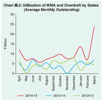 3.21 Special WMA is a secured advance linked to the investments made by state governments in central government securities, including investments in the consolidated sinking fund (CSF) and the guarantee redemption fund (GRF). The nomenclature of the special WMA was changed to special drawing facility from June 23, 2014 by amending the agreements the states have entered with the Reserve Bank. | Table III.14: Key Deficit Indicators in 2014-15* | | (Per cent of GSDP) | | Item | Budget Estimates | Revised Estimates | | 1 | 2 | 3 | | Revenue Deficit | -0.5 | 0.1 | | Gross Fiscal Deficit | 2.6 | 3.1 | | Primary Deficit | 0.8 | 1.4 | *: Provisional data based on budget documents for 2015-16 for 17 state governments
Note: Negative sign indicates surplus | 6. Conclusion 3.22 The post-crisis fiscal consolidation experience of states indicates erosion of revenue surpluses particularly in 2013-14(RE). Although the fiscal deficit at the consolidated level remained within the target set by FC-XIII during the period under review, state level targets were not met by some states. GFD was budgeted to be contained at 2.3 per cent of GDP in 2014-15, aided by a sharp increase in the revenue surplus. Revenue receipts were budgeted to record higher growth mainly on account of increase in current transfers from the centre, particularly grants, in view of routing of CSS funds through the state budgets from the fiscal year 2014-15. 3.23 Based on the latest budget documents of 17 states, which accounted for 88 per cent of both the non-debt receipts and total expenditure in 2014-15(BE), the revised estimates for 2014-15 indicates deterioration in the deficit indicators as compared to the budget estimates (Table III.14). Creating fiscal space for higher capital outlays, improving the quality of fiscal consolidation and containing the debt-GDP ratio of the states are crucial to improving finances of the states.
|