Kumudini Hajra, Rajeev Jain and Dhirendra Gajbhiye*

The paper attempts to explore the phenomenon of surplus cash balances at the State level. Apart from discussing the developments that led the States to build-up their cash surplus positions, the paper identifies the determinants of surplus cash balance across States. The reason for accumulating cash surplus appears to be largely precautionary for meeting any liability of big magnitude. The paper finds that from the revenue side, own tax revenue and current transfers from Centre are determining factors while compression in revenue expenditure also explains the build-up of cash surplus across States. It is observed that some States could have spent more on capital outlay instead of accumulating cash surplus. The paper also suggests some alternative options for investment of cash balances along with measures for better cash management.

I. INTRODUCTION

State finances in India have undergone some significant changes in recent years. Although fiscal reforms at the State level have been an important component of economic policy reforms, the finances of the States continued to deteriorate even during the 1990s. It was in this backdrop that the Eleventh Finance Commission recommended a fiscal reform incentive scheme. The Twelfth Finance Commission (TFC) too evolved schemes for fiscal correction of states. The Government of India also moved swiftly to facilitate fiscal reforms at the State level and the idea of ‘incentivising reforms’ took roots (World Bank, 2004). In recent years, a number of important initiatives have been undertaken in the form of State level Fiscal Responsibility Legislations (FRLs) and various institutional reforms along with reforms relating to market borrowing programme.

As a result of various initiatives, States have recorded an average revenue surplus of 0.5 per cent of GDP during 2006-07 and 2008-09. Reflecting the improvement in revenue balance, the average gross fiscal deficit (GFD) as a percentage to GDP has also been lower during this period as compared with the earlier years. The outstanding liabilities of the State Governments as a percentage to GDP at 32.7 per cent as at end-March 2005 have also consistently fallen thereafter. Some incipient signs of a compositional shift are also evident in the financing pattern of GFD at the State level. For instance, market borrowings have emerged as the major source of financing of GFD since 2007-08 as against special securities issued to National Small Saving Fund (NSSF), which used to be the major source of financing of GFD during the past few years. A comparison of State finances vis-à-vis restructuring plan suggested by the TFC shows that at the consolidated level, States have over - achieved the deficit and debt targets much ahead of the time-frame stipulated by the TFC. However, the worrisome factor remains the quality of fiscal correction and consolidation as States were unable to scale up their capital expenditure.

Improvement in fiscal situation in recent years has been achieved by pursuing the fiscal correction and consolidation process under a rule based fiscal framework. All but two States, viz., West Bengal and Sikkim have enacted the FRLs. The efforts of State Governments towards reducing fiscal imbalances were aided by larger devolution and transfers from the Centre based on TFC recommendations along with improvement in tax buoyancy on the strength of macroeconomic fundamentals. All States have implemented value added tax (VAT) in lieu of sales tax, which turned out to be a buoyant source of revenue for the State Governments. Furthermore, the Debt Swap Scheme during 2002-05 along with incentives provided by the TFC under the Debt Consolidation and Relief Facility helped States in restructuring their liabilities and led to lower interest burden as well as reduction in their debt obligations. However, situation with regard to debt remains precarious in some States which needs to be addressed on a priority basis.

Alongside the improvement in fiscal position of States, there has been a build-up of cash balances with them. Some part of these cash balances has arisen on account of temporary liquidity mismatches and reflects a tendency on the part of the States to avoid recourse to Ways and Means (WMA)/overdraft (OD). Realising the need for meeting any prospective exigency, States seem to have taken recourse to build up cash surplus as a precautionary measure, instead of resorting to WMAs/OD (Statement 1).

The surplus cash balances of States have persisted since 2004-05 and stood at Rs.1,01,969 crore as at end-March, 2009. Such high magnitude of cash balances raises issues regarding the cash management by State Governments. The build-up of surplus cash balances was initially contributed by excessive autonomous inflow of NSSF collections. For instance, during 2004-05, NSSF accounted for 72.3 per cent of total incremental liabilities of the State Governments. However, of which only 76.7 per cent was used for financing of GFD (Table 1). This phenomenon continued during 2006-07 as well. Despite a sharp decline in NSSF inflows in recent years, the phenomenon has persisted mainly on account of various factors, inter alia, initiation of rule-based fiscal regime, larger devolution and transfers from the Centre based on the recommendations of the Twelfth Finance Commission (TFC) along with improvement in tax buoyancy on the strength of macroeconomic fundamentals.

The build-up in the surplus cash balances has implications for (i) revenue balances of States, (ii) Centre’s cash management and (iii) open market operations of the Reserve Bank.

Against this background, the objective of this paper is three-fold. First, an attempt is made to analyse whether all the States contributed uniformly in building up of high level of surplus cash balances or it is limited to a few States. Second objective is to make an attempt to quantify the factors responsible for high surplus cash balances across States. The objective is to examine whether persistence of cash balances in recent years has been the result of structural changes that have taken place during the process of fiscal correction and consolidation at the State level. Third, what could be the alternative investment options for surplus cash balances?

In the Indian context, even though the factors responsible for building up of high surplus cash balances across States are well understood, it is important to quantify the contribution of various factors. Keeping this in view, the present Study attempts to examine the determinants of surplus cash balances in panel data framework. Panel data analysis endows regression analysis with both a spatial and temporal dimension. In the present study, the spatial dimension pertains to a set of cross-sectional units of States. This will help us in examining the underlying factors behind the build-up of surplus cash balances across the States. In section II, cross-country experiences with regard to cash balances of national/sub-national governments are discussed. Section III discusses the trend in surplus cash balances. Major factors responsible for build-up in cash balances are discussed in Section IV along with empirical analysis for quantifying the determinants using balanced panel of 28 States for the period 1999-2000 to 2008-09. In Section V, the issue with regard to cost of maintaining high cash balances by States is discussed. In Section VI, an attempt is made to examine the possible alternative uses of surplus cash balances. Section VII contains concluding observations.

II. SURPLUS CASH MANAGEMENT: INTERNATIONAL EXPERIENCE

Government cash management has been given less attention than government debt management by the international agencies, by governments themselves, and by consultants and academics (Williams, 2004). Emphasising on time-value of money, Storkey (2003) argues that cash management is “having the right amount of money in the right place and time to meet the government’s obligations in the most cost-effective way.” Thus, cash management of the government should focus not only on funding of expenditures and meeting the obligations in a timely manner but it should also be cost-effective and efficient.

Cross-country studies have often emphasised on cash management at the national government level rather at the State government level. Lienert (2008) finds that in advanced countries, when there are temporary cash shortages or surpluses, the government’s cash manager, who is monitoring the consolidated balances of all government accounts on a daily basis, borrows or lends to the financial markets. Temporary surpluses in the treasury single account (TSA) are invested in interest-bearing instruments, usually with full collateral so as to minimise risk. There is increasing participation of treasuries in secondary markets for government securities, with the twin objectives of maximising returns on available balances and avoiding timing mismatches. In many euro countries, the government usually sets an end-of-day balance target for its single treasury accounts. Cash managers in these countries usually actively invest the excess balance or borrow in the financial markets to reach the balance target (Mu, 2006). In EU countries, treasuries are often active in repo. In the case of France, active cash management of the national government is done by way of investing temporary surplus cash in the account at the highest yield and safety while maintaining a credit balance in the account. Several other countries have established a daily operating target for the balance in the TSA, with any temporary surpluses actively invested in financial markets. However, countries like Australia do not have an explicit daily operating target and the cash management office aims to reduce the daily fluctuations in the TSA balance. In the case of Australia, simple cash management model is in place. Accordingly, structural surpluses are placed with the central bank on longer-term interest rates based on the preset agreement between the Ministry of Finance and the central bank. In Finland, during the phase of high level of liquidity, the cash funds are invested in the financial markets, mainly in short-term securities and covered bonds. In New Zealand, departments negotiate their annual cash requirements with the treasury, and pay an interest-rate penalty if they run out of cash, or earn interest on their surplus funds. In parallel, the New Zealand Debt Management Office (NZDMO), which is the branch of the treasury and responsible for cash and debt management, sweeps department bank accounts each evening and invests the surplus in the overnight money market (ADB, 1999). In Canada, the cash balances of the Central Government are auctioned in a competitive auction twice a day to a select set of participants. The participants’ auction limits (collateralised and uncollateralised) are decided on the basis of their credit rating. In the case of USA, the treasury maintains a stable working balance in its Federal Reserve Bank accounts and parks the remainder of its cash in private depository institutions until needed. In South Africa, all surplus cash of the exchequer is deposited daily into the tax and loan accounts at the four major commercial banks.

As far as cash management at the sub-national level is concerned, there are only a few studies. Recognising the fact that security of principal is crucial for government, all States in the USA keep a portion of investment of idle cash balance in permissible securities. The nature of cash balances invested by State governments can be classified into three types, viz., temporary surplus, long-term surplus and pooled surplus. Temporary surplus results from lag between collection and spending and is expended within a year. The concept of long-term cash surplus held by the States for a year or more is often associated with trusts, pension or debt serviced funds while pooled cash surplus results from pooling of cash balances from the separate funds or even multiple governments (Rabin, 2003).

The safety or credit risk of issuer of these securities, as well as liquidity and marketability are the major factors that are looked into before choosing these instruments (Brick, Baker and Haslem, 1986). In Indonesia, sub-national governments use bank deposits to invest their surplus cash funds (Lewis, 2008).

III. SURPLUS CASH BALANCES: TREND ANALYSIS

State finances have been witnessing an unusual trend in the recent past in terms of availment of WMA/OD from the Reserve Bank of India and surplus cash balances. During the late 1990s and in the beginning of 2000s, State Governments used to avail WMA/OD quite often (with the objective of covering temporary mismatches in the cash flows of their receipts and payments) and level of their surplus cash balance was quite meager. However, the buoyancy in small saving collections over the last few years and the automatic channelisation of these funds to the States has meant that State Governments’ borrowings through internal debt and public account are more than the amount required for financing their GFD. On top of that, there has been significant improvement in revenue augmentation at the State level. This gets reflected in large surplus cash balances maintained by most of the State Governments in the form of investments in 14-Day Intermediate and Auction Treasury Bills.

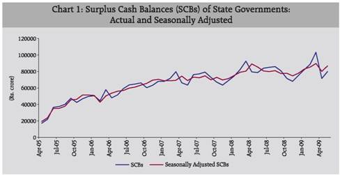
An increasing trend in cash balances of States can be observed particularly since 2004-05. Since the beginning of 2005-06, the cash surplus balance of all States has grown at a compound annual growth rate of 57 per cent. Not surprisingly, a majority of the States stopped seeking short-term liquidity support from the Reserve Bank through WMA window and OD facility. The cash surplus adjusted for seasonality shows that there are significant spikes in the fourth quarter of every year. It is perhaps on account of the fact that most States tend to exhaust their allocated market borrowing limits during the last quarter of the year and thereby build-up surplus cash position to be used for the first quarter of the next financial year when cash inflow generally remains low, while heavy spending by Government departments takes place (Chart 1).

Having identified the factors that are apparently responsible, in accounting sense, for building of surplus cash position at the State level, an important question remains as to why the States accumulate surplus cash balances instead of spending. The reason appears to be that States intend to avoid resorting to ‘WMAs’ or ‘Overdraft’ in the event of major payment obligations coming forth and be labeled as poor performing States. In order to avoid any shortage of liquidity for making any lump-sum payment, they might have built-up surplus cash position in recent years.

State-wise analysis shows that 13 states which accounted for around 90 per cent of total outstanding cash balances during 2005-06 and 2007-08 were Uttar Pradesh, Tamil Nadu, Gujarat, Haryana, Maharashtra, Orissa, Karnataka, Andhra Pradesh, Assam, Rajasthan, Madhya Pradesh, Chhattisgarh and Bihar. However, the volume and nature of surplus cash balances varies widely across States. Among these States, there are some States like Haryana, Maharashtra, Orissa, Chhattisgarh, Assam, Karnataka and Tamil Nadu which had significantly lower GFD as percentage to Gross State Domestic Product (GSDP) during this period than the prescribed norm of 3 per cent under their FRLs. This indicates that these States did have more space to incur capital outlay without violating FRL norm but they preferred to accumulate cash surplus perhaps for precautionary purposes. In fact, in some of these States, capital outlay as a percentage to GSDP has either declined or remained stable in recent years. This is worrisome and can have implications for long-term growth prospects of States (Table 2).

There is another set of States comprising Uttar Pradesh, Rajasthan, Bihar and Andhra Pradesh, which appear to have built-up surplus cash balances, given their high debt-GSDP and GFD-GSDP ratios. Since such States are constrained to spend more as capital outlay, they might be envisaging repaying a part of their high cost debt out of such balances in order to attain a sustainable debt-GSDP ratio as has been done by Orissa. For such States, another option could have been to finance their GFD by drawing down their cash balances rather than by resorting to excessive borrowings.

IV.  DETERMINANTS OF SURPLUS CASH BALANCES: PANEL DATA ANALYSIS

As mentioned above, the increase in Central transfers to States, improved buoyancy in own tax revenues, the availability of debt relief based on recommendations of the TFC, and the buoyancy of small savings collection might have resulted in a built up of surplus cash position by State governments and low or non-utilisation of WMAs. Kishore and Prasad (2007) argue that the large cash surpluses imply that States have over-borrowed for funding the GFD, or have underestimated their GFDs, or have breached their net borrowing ceilings on account of excess inflows from the NSSF. Issac and Ramakumar (2006) argue that the constraint on expenditure imposed by the FRLs enacted by most State Governments led to the cash surplus phenomenon. In this section, an attempt is made to explain the factors that have been responsible for accumulation of cash surplus at the State level, which could result either from the augmentation on receipt side (both revenue and capital) or compression on expenditure side (both revenue and capital).

The explanatory variables that are used in panel data analysis for explaining surplus cash balances of States are given below:

SCB        : Surplus Cash Balance
OTR        : Own Tax Revenue
CT           : Current Transfers from the Centre
RE          : Revenue Expenditure
GFDEXP    : GFD Expenditure
OB          : Over Borrowing

OTR represents own tax revenue of States which as a percentage to GDP has steadily improved from 5.8 per cent in 2004-05 to 6.2 per cent in 2008-09 (BE). Augmentation in OTR in the current decade has been mainly on account of improved revenue generation from States’ sales tax/VAT and stamp and registration fees. It is hypothesised that steady improvement in OTR might have eased financial position of States and facilitated them in building surplus cash balances.

CT represents current transfers to States which includes share in Central taxes and grants from Centre. This is another significant factor that has made revenue account position of the States comfortable. CT as a percentage to GDP improved from 4.3 per cent in 2004-05 to 5.8 per cent in 2008-09 (BE).

RE represents revenue expenditure. In the post-FRL period, there has been some rationalisation in revenue expenditure. As a result, at the consolidated level, RE as a percentage to GDP declined from 13.5 per cent in 2003-04 to 12.7 per cent in 2008-09 (BE). It is often argued that enactment of FRLs at the State level, envisaging to eliminate revenue deficits by 2008-09, forced them to reduce their revenue expenditure which in turn has implications for their cash position as well.

OB represents over borrowing over and above their GFD requirement. It is observed that some States tend to borrow more than their GFD financing requirements, if one takes into account borrowings from all sources. Given the fact that States are not allowed to carry forward their unutilsed portion of allocated market borrowings to the next financial year, there might be a tendency among the States to generate additional fiscal space for future by raising the entire amount of allocated borrowings, which otherwise are not required for financing their GFD. This might be due to the fact that market borrowings raised in previous years are used as a basis for deciding the market borrowing program of States for the forthcoming year. Given this, States may like to raise the entire amount as per their gross allocation.

GFDEXP representing GFD expenditure including revenue expenditure, capital outlay and loans and advances (net of recoveries). During 2005-06 to 2008-09, GFDEXP was stagnant at the same level of 15.2 which was observed during 2000-01 to 2004-05.

Panel data estimation models mainly include the constant coefficient (pooled), the fixed effects (FE) and the random effects (RE) regression models. Whereas the pooled regression model assumes that the different cross sections are undifferentiated, the fixed and random effects models take into account the differences. Under the FE model, differences that arise among the cross sections are accounted for by fitting cross sectional intercepts [the Least Squares Dummy Variable (LSDV) Model which assumes that the heterogeneity between cross sections can be accounted for this fitted intercept]. Under RE model, differences are accounted for by appending a cross section specific error term that is in addition to the least squares error component of an estimating equation. In this section, estimated results are reported based on all the three models. Hausman Specification Test (Hausman, 1978) is used to test and compare the fixed and random effects estimates of coefficients. Generally, the random effects model is required to be used if the panel data comprise N observations drawn randomly from a large population, whereas the fixed effects model is more appropriate when focusing on a specific set of N individuals that are not randomly selected from some large population. Since in the present paper, the States are not randomly drawn from the population and there is no selectivity bias, the fixed effects model appears to be more suitable for the analysis.

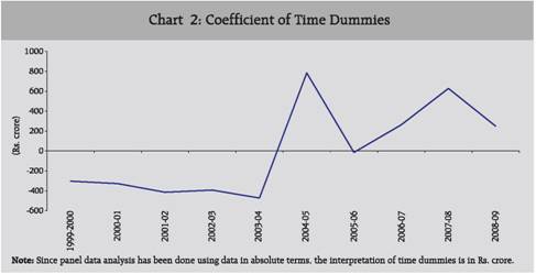
Before we discuss parameter estimates, the issue is whether there is an evidence of cross-section (State) and time effects. To examine this, the joint significance of the firm and/or the time dummy variables in the fixed effects specification is tested. It is found that under FE Model, cross-section (State) specific fixed effects are statistically significant at 1 per cent while period specific fixed effects are statistically insignificant (Table 3). In other words, change in surplus cash balances across the different years on account of unobserved factors (i.e., other than included variables, viz., OTR, CT, RE and OB), is not statistically significant. However, the pattern as shown by the time dummies for 2000-09 shows a systematic shift in surplus cash balances of States in recent years due to unobservable factors but their contribution in explaining them is not statistically significant (Chart 2). Given the evidence that period effects under FE model are non-existent, the paper focuses on explaining the surplus cash balances using FE model with cross section (State) effects.¹

Empirical analysis using panel data of 26 States² for 10 years (1999-2000 to 2008-09) shows that all the variables turned out to be statistically significant at 1 per cent as per a priori expectations (Table 4). As was hypothesised, revenue augmentation efforts reflected in improvement in OTR have positively impacted the cash balances. It can be observed that coefficient of OTR in all models is highest and statistically significant at 1 per cent. It can be interpreted as one rupee change in OTR leads to approximately 50 paise increase in cash balances of States. From the revenue side, current transfers from Centre have also helped States to build-up surplus cash balances, as the coefficient of CT is statistically significant at 1 per cent in all models. As far as compression in revenue expenditure is concerned, it also contributed to accumulation of cash surplus across States. As shown in Table 3, compression in revenue expenditure by one rupee leads to an increase in cash balances by around 25-30 paise. As was expected, over-borrowing by States over and above their GFD has also impacted cash balances positively as the coefficient of OB turned out to be statistically significant in the FE model.

In an alternative equation using GFD expenditure (GFDEXP) instead of RE, it is found that coefficients of OTR and CT continue to remain significant under all models, while the coefficient of OB turns statistically insignificant. However, coefficient of GFDEXP turns out to be virtually the same as that of RE in the earlier equation. It shows that from the expenditure side, compression in RE largely contributed to cash balances of States (Table 5). The negative coefficients of RE and GFDEXP appear to be an outcome of the implicit expenditure limits assumed by States with a view to achieve their respective RD and GFD targets as envisaged under FRLs. It is quite possible that States have achieved fiscal prudence by limiting their expenditure, particularly revenue expenditure, which along with revenue augmentation measures appear to have facilitated the build-up of surplus cash balances. As mentioned in the previous section, some States are found to be extra cautious even though their GFD is significantly lower than the prescribed level of 3 per cent of GSDP. If the expenditure rationalisation undertaken by States is through curtailing the development expenditure of capital nature, it should not be construed as a healthy development. It seems that States tend to accumulate cash balances by generating revenue surplus instead of revenue balance as suggested by their respective FRLs.

As far as State-wise significance of variables is concerned, Table 6 shows that OTR has impacted cash balances of 12 States as state-specific coefficient of OTR is statistically significant at 1 per cent. Similarly, current transfers from Centre seem to have impacted cash balances of 14 States, particularly the special category States. Compression in revenue expenditure has impacted cash balance in case of 10 States as their respective coefficients were negative and statistically significant. The coefficient of OB seems to have been statistically significant only in case of two States. GFDEXP used instead of RE in an alternative equation turns out to be statistically significant in 10 States.

In order to examine the efficacy of fixed effect model, redundant fixed effects test is used, which evaluates the statistical significance of the estimated fixed effects. It strongly rejects the null hypothesis that the fixed effects are redundant. In other words, under FE model, heterogeneity across States in terms of cash surplus accumulation captured through different intercepts for each State is statistically significant. In short, apart from the explanatory variables, the presence of State-specific unobservable factors, captured through (cross section fixed effects), impacting their cash balances cannot be ruled out. In order to test closeness of the coefficients from a random effects pool equation to the corresponding fixed effects specification, Hausman test is conducted. The result shows that two out of four coefficients estimated by the efficient random effects estimator are not the same as the ones estimated by the consistent fixed effects estimator. FE model appears to be better in explaining the surplus cash balances across States with explanatory power of 0.80 than other models.

V. INVESTMENT OF CASH SURPLUS: AN ISSUE FOR STATES AND CENTRE

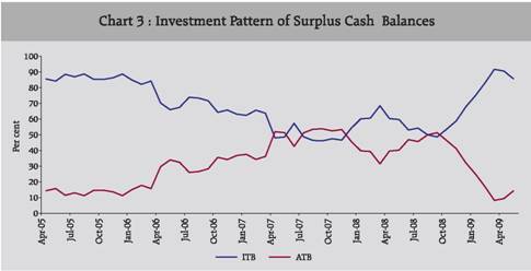
Surplus cash balance of a State beyond a level indicated by it is automatically invested in 14-day intermediate Treasury bills (ITBs), which presently carry a rate of interest of 5.0 per cent. This rate is significantly lower than that paid on the market borrowings by the States and the small savings. The States are also free to participate in 14-day and 91-day Treasury bills auctions as non-competitive bidders for investment of their durable surplus cash balances. However, States are not allowed to invest in dated Central Government securities. The interest rate on 14-day intermediate Treasury Bills has been fixed at 1 percentage point below the Bank Rate with effect from 2001-02 as against 3 percentage points earlier. Since Auction Treasury Bills (ATBs) fetched higher yield than the 14-day ITBs, some shift from ITBs to ATBs was observed till September 2008 (Chart 3). This could be attributed to the perceived durability of surplus balances with the State Governments and relatively higher yield (around 7-8 per cent) in ATBs. However, with the softening of interest rate in subsequent months, the trend appears to have reversed in favour of ITBs.

During 2005-09, the Government of India approximately received a return of 6.44 per cent³ on its investments (made out of its surplus cash balances). It, however, ended up paying 5 per cent on the investments in ITBs and about 6.64 per cent (based on the weighted average of auction cut-off for 91- day Treasury bills) on investments in ATBs. The year wise simple average of 91-day T-bill auction cut-offs works out to 5.68 per cent, 6.63 per cent, 7.12 per cent and 7.10 per cent, respectively for 2005-06, 2006-07, 2007-08 and 2008-09 (the recent 91-day auction on May 13, 2009 had a cut-off of 3.28 per cent). Due to the differences in returns, there could be a negative carry for the Central Government at times if the States choose to invest more in favour of ATB when the returns are higher on ATBs than on ITBs. There are two issues associated with regard to the cost borne by the Centre. First, Centre has no discretion over the investment by States in ITBs and ATBs and has to pay the cost even when it does not need cash. Second, Centre has to pay higher interest as States switch over from ITBs to ATBs to get more favorable return.

Faced with the accumulation of surplus cash balances and a negative spread earned on the investment of such balances, State Governments have been feeling the need of reviewing the existing investment mechanism of their cash balances. States can invest the surplus cash balance only in ITBs or ATBs. Since the States earn a lower rate of return on these investments, instead of over-borrowing, it is argued that States could have used surplus cash balances to meet their GFD financing requirement. This could have mitigated the additional interest burden arising out of negative carry on cash balances. In fact, the high cost involved in investing cash balances prompted some State Governments to utilise their surplus cash balances to retire outstanding debt. In recent years, States have approached the Reserve Bank to arrange for the buy-back of their outstanding State Development Loans (SDLs). Accordingly, the Reserve Bank has formulated a general scheme for the buy-back of SDLs with the concurrence of Government of India. So far, buy-back auctions have been conducted for two State Governments (viz., Orissa and Rajasthan) and a total amount of Rs.479.07 crore of SDLs has been bought back.

Another issue is with regard to volatility in surplus cash balances. Since the surplus cash balances are automatically invested in 14-day ITBs and ATBs of the Central Government, they impart volatility to the cash balances of the Government of India. During 2005-06 to 2008-09, the Central Government’s cash position showed wide fluctuations, partly contributed by the variations in the States’ investments in ATBs and ITBs. In fact, surplus cash position at the State level has become a source of funding for the Central Government. It is evident from the fact that in the absence of surplus cash balance at the State level, the Centre would have been in WMAs during 2005-06 and 2008-09. Despite this, surplus cash position of States cannot be a dependable source of funds for the Centre. Uncertainty over the movement of Government cash balances, partly on account of uncertainty of cash position of State Governments may complicate the management of liquidity necessitating Reserve Bank’s intervention.

With an upsurge in cash balances, another issue that arises is with regard to its optimum investment. Under the present investment framework for surplus cash balances, there are not much investment options for States. It is often argued that the State Governments might need alternative investment options to park their surplus funds and may require setting up debt units and developing necessary expertise for cash and investment management.

VI. ALTERNATIVE OPTIONS AND MEASURES FOR BETTER CASH MANAGEMENT

The upsurge in the surplus cash balances at the State Government level since the middle of 2004-05 has posed newer challenges to financial and cash management of State Governments. It seems that States build-up cash balances for precautionary motive so as to avoid recourse to overdraft on account of any exigency of high magnitude. Furthermore, States do not want to be labeled as “overdraft” States which leads them to accumulate cash surplus even though it is a costly option. As a result, during 2008-09, the average utilisation of normal WMA, special WMA and overdrafts by the States remained low reflecting improvement in the overall cash position resulting in build-up of high level of surplus cash balances by most of the State Governments.

As regards the investment of cash surplus, the Bezbaruah Committee on WMA to State Governments (2005) had recommended that States which had not availed any WMA in the immediate preceding period of 90 consecutive days, should be allowed to invest in dated Central Government securities. However, this recommendation has not been accepted so far. Another usage of surplus cash balances could be at the time of cyclical downturn, when States can drawdown their surplus balances to supplement their expenditure programmes as counter-cyclical measures. During the current phase of macroeconomic slowdown, it is widely expected that States will tend to spend more to boost their domestic demand while there is considerable uncertainty on tax collection front, both at Centre and State level. Thus, the high level of cash surplus accumulated at the State level in recent years provides some headroom to withstand pressure on their finances. As a result, the surplus cash balances at the State level may wipe out during the current phase of slowdown. In fact, the level of surplus cash balances of States has decreased from the highest level of Rs.1,19,676 crore as on March 20, 2009 to Rs. 79,506 crore as on June 26, 2009. States may further resort to drawdown of their cash balances to meet their spending obligations arisen on account of implementation of recommendations of sixth Central Pay Commission and stimulus measures. If unaddressed, the issue may re-emerge once the economy gathers growth momentum and fiscal distress for States eases. Given the fact that holding of surplus cash balances has been a costly option for States and also makes the Central Government cash balances volatile, there should be some framework with regard to investment of cash balances.

In order to deal with the concern of high cost involved in accumulation of cash balances, one of the policy options could be to link the rate of return on 14-day ITBs to other policy rates like reverse repo rate. With the parity in ITB rate and principal signaling policy rate, i.e., reverse repo rate, the issue of forced cost imposed on the States would get addressed. This will also encourage States to build the capacity of projecting their cash flows on account of receipts and expenditures and rationalise their surplus cash balances with the purpose of minimising the negative carry.

It is evident from the empirical analysis that over-borrowing by States also contributes positively to the accumulation of surplus cash balances albeit not significantly. At present, States are not allowed to carry forward their unborrowed amount to the next financial year. In order to build-up their precautionary cash balances, they tend to borrow over and above their GFD requirements. To deal with this issue, States may be allowed to carry forward a part of their allocated but unborrowed amounts to the next financial year. This will not only make the borrowing programme of States more need-based but also provide States the adequate flexibility to borrow during opportune times in a cost effective manner. During the boom period, States may borrow less and save their unborrowed quota for downturn phase when the need to spend more arises to boost the economy. In other words, such an arrangement would make the States more confident to undertake counter-cyclical fiscal policy.

As mentioned above, since States do not want to be labeled as “overdraft” States, they seem to be accumulating cash surplus as a precautionary measure even though it is a costly option for them. In order to deter the States to accumulate unwarranted cash surplus, a possible option could be a significant revision in WMA limits. Substantial upward revision in WMA limits may address their concern of frequently going into overdraft. Sufficient WMA limits along with changed nomenclature may discourage the States to build-up cash surplus unnecessarily.

From the States’ side, the ultimate goal should be the development of better cash management capacity. State Governments should have some effective forecasting and monitoring mechanism for their cash inflow and outflows. Effective cash management is possible only if there are skills and capacity to record, monitor, and project short-term inflows and outflows into the TSA, as has been the practice in most of the advanced economies. First issue is with regard to realistic forecast of cash flows to facilitate effective cash management. For this purpose, they can set up a special unit with specialised Staff for facilitating the preparation and updating of short-term cash projections and maintaining databases of historical cash-flow trends. Second issue is the need for close coordination of all government entities. In this context, it may be noted that in advanced countries, high quality, timely and comprehensive data on government cash transactions are usually readily available in the government’s accounting system. For short-term cash projections, all relevant entities contribute to the provision of necessary data. Information sharing networks have been set up and there are clear understandings of the responsibilities of government entities for different aspects of cash management. For this purpose, States should encourage coordination among the State entities that collect revenue and expend funds. Better timing of decisions involving major expenditures and rationalising the number of bank accounts may also help them in rationalising the use of cash surplus.

VII. CONCLUDING OBSERVATIONS

The paper finds that around 90 per cent of surplus cash balances have been contributed by 13 States, mainly the non-special category States. Of these, some States have already achieved their deficit and debt targets well ahead of the stipulated time as prescribed by the TFC. Despite the improvement observed in terms of deficit and debt indicators in a few States, their capital outlay as a percentage of GSDP is either stagnant or on a lower side. It can be inferred that such States, having debt-GSDP ratio within the limit of 30.8 per cent (prescribed by TFC), could have spent more on capital outlay without violating the GFD-GSDP norm of 3 per cent instead of accumulating cash balances. It indicates that either there is no further capacity in the States to absorb further capital spending or they are too conservative in their approach. Empirical analysis shows that build-up of cash balances across States has been an outcome of States’ own efforts to augment tax revenues and exogenous factors including larger devolution and transfers by the TFC through shareable Central taxes and grants. Although variables, viz., OTR, CT and RE enabled the build-up of surplus cash balances in recent years, the contribution of revenue receipt components is larger. The cross-section heterogeneity arising out of unobservable State specific circumstances is also important in explaining the State-wise cash surplus. In order to address the issue of cost involved in maintaining cash balances, investment options and rate of return thereon need to be explored. Further, States should make serious efforts towards building up the capacity for better cash management. It is suggested that apart from greater coordination among the Government entities required for making realistic assessment of cash needs, States should also attempt to avoid unwarranted build-up of cash surplus by adopting advanced forecasting and monitoring mechanism keeping in view the best practices across advanced economies. As a result of effective cash management and better synchronisation of cash inflows and outflows, States may be able to minimise their borrowing requirement. This may also help, to some extent, to curb unwarranted build-up of cash surpluses by the States which has implications not only for Centre’s cash balances but also for monetary policy.

References:

Bank of Canada (2000), ‘‘Proposed Revisions to the Rules Pertaining to Auctions of Receiver General Term Deposits’’, Bank of Canada Discussion Paper available at http://www.bankofcanada.ca/en/pdf/cash-bal.pdf

John R. Brick, H. Kent Baker and John A. Haslem (1986), Financial Markets: Instruments and Concepts, 2nd. ed., Reston, VA : Reston Publishing.

Garbade, Kenneth D, John C. Partlan and Paul J. Santoro (2004), ‘‘Recent Innovations in Treasury Cash Management’’, Current Issues in Economics and Finance, Vol.10, No. 11, Federal Reserve Bank of New York.

Isaac, T. M. Thomas and R. Ramakumar (2006), “Why Do the States Not Spend? An Exploration of the Phenomenon of Cash Surpluses and the FRBM Legislation”, Economic and Political Weekly, Vol. 41, No. 48, December 2.

Kishore, Adarsh and A. Prasad (2007), “Indian Subnational Finances: Recent Performance”, IMF Working Paper No. WP/07/205, International Monetary Fund.

Lewis, B.D. (2008), “A Note on the Indonesian Sub-National Government Surplus, 2001-2006”, at http://www.dsfindonesia.org/userfiles/Surplus%2010608%20BL.pdf

Lienert, Ian (2008), “Cash Management”, PFM Technical Guidance Note No.5, International Monetary Fund, February.

Mu, Yibin (2006), “Government Cash Management: Good Practice & Capacity-building Framework”, Financial Sector Discussion Series, World Bank.

Rabin, Jack (2003), Encyclopedia of public administration and public policy, Published by Marcel Dekker.

Reserve Bank of India (2005), Report of the Advisory Committee on Ways and Means Advances to State Governments, (Chairman: M.P.Bezbaruah) October 2005.

Reserve Bank of India (2008), State Finances: A Study of Budgets of 2008-09, Mumbai.

Schiavo-Campo, Salvatore and Daniel Tommasi (1999), “Managing Government Expenditure: Cash Management and the Treasury Function”, Asian Development Bank.

Storkey, Ian (2003), “Government Cash and Treasury Management Reform”, Asian Development Bank, Governance Brief, Issue 7-2003, available at www.asiandevbank.org/Documents/Periodicals/GB/GovernanceBrief07.pdf.

Williams, Mike (2004), “Government Cash Management Good and Bad – Practice”, available at http://treasury.worldbank.org/web/pdf/williams_technote.pdf.

World Bank (2004), “The Government of India also moved swiftly to facilitate fiscal reforms at the State level” Report No. 28849-IN,November 2004.

* Authors are Director, Assistant Adviser and Research Officer, respectively in the Department of Economic Analysis and Policy of Reserve Bank of India. Authors thank Shri B. M. Misra, Advisor for his encouragement and support. Views are personal and not of the institution they belong to.
¹ Results from random effects specification are also reported for comparison.
² Jammu and Kashmir and Sikkim are not included.
³ Based on indicative list of earmarked securities amounting to Rs.50,000 crore.