by Sukhbir Singh and Vishal Maurya^{^}

This article introduces a new off-site monitoring system for surveys (OMOSYS) for ensuring data quality in extensive field surveys. The system employs new locational measures for identification of doubtful survey responses by utilising geographic information system (GIS) data from computer-assisted personal interviewing (CAPI) instruments. The model driven indicator (MDI) and fixed control indicator (FCI) approaches developed in this article help identify doubtful cases in a flexible manner without any manual intervention. The OMOSYS facilitates targeted tracking of field visits for maximising efficiency and maintaining survey quality in diverse geographical domains, which are vital for time-sensitive and resource-constrained surveys.

Introduction

Surveys play a pivotal role in organised societies that rely on information as input in decision-making and their subsequent monitoring. Accuracy, reliability, and timeliness of survey data thus become critical, given their far-reaching implications in the policy-making process across diverse policy domains. In many areas of economic conditions enquiries, in-person interviews although more resource-intensive but have distinct advantages over telephonic and on-line surveys in terms of obtaining targeted responses, better understanding through human interaction and higher response rate. In addition to checking of a survey’s primary data, quality assurance measures often involve physical follow-up visits to surveyed locations by quality controllers / coordinators to validate survey responses on a sample basis. These on-site visits not only ensure proper compliance with instructions and design of the survey by investigators but also offer first-hand enriching experience, which proves instrumental in streamlining the training of the investigators, study survey design as well as refine survey questionnaire/explanations.

In a large and diverse country like India, conducting nation-wide surveys with stringent timelines becomes challenging in terms of ensuring on-ground adherence of survey design and coverage instructions, as the expanse requiring field visit by investigators becomes very large, and issues arise, especially with respect to compliance to the instructions by investigators or genuineness of respondents. This can lead to diminished likelihood of identifying locations during field visits for response validation. The challenge would be especially serious in remote areas where low probability of follow-up field verification can potentially prompt some investigators to conduct surveys at more convenient locations away from the targeted spot, which would compromise the intended design instructions and the desired quality of the survey data.

To address these challenges, innovative and pragmatic methods have been developed here by leveraging the potential of locational information of respondents captured by the instrument used to conduct the survey. This geographic information system (GIS) data in the form of geo-coordinates (viz., latitude and longitude) has been utilised to develop an off-site monitoring system for surveys (OMOSYS), which tracks survey execution on a near real-time basis. Statistical methods are specifically designed for the purpose along with processes, which effectively implement and operationalise these methods.

The article provides a detailed account of the OMOSYS along with illustrations of its use in household surveys conducted by the Reserve Bank of India (RBI). The article is structured into five sections. Following the introduction, Section II delves into the general data quality assurance (QA) processes employed in surveys and highlights the associated challenges. Section III provides comprehensive information of the OMOSYS utilising GIS information, offering a solution to the identified issues. Section IV demonstrates the application of the OMOSYS through real cases and synthetic data, providing practical insights. The concluding section summarises the findings and recommendations.

II. Quality Assurance Process in Surveys

Field surveys gather data by firstly designing sampling frames, where suitable sampling scheme is employed for selecting first stage units (FSUs) and second stage units (SSUs), and robust data quality assurance (QA) methods are used. For instance, in the context of urban household surveys conducted by the Reserve Bank of India (RBI), such as Inflation Expectations Survey of Households (IESH) and Consumer Confidence Survey (CCS), the polling booths/ wards serve as the FSUs. These FSUs form the basis for obtaining subsequent household-level responses, where randomisation of respondents is crucial to avoid biased results (RBI, 2018, 2019). Selecting respondents in very close proximity with each other may result in highly correlated responses, potentially leading to biased and skewed results. Additionally, if respondents are located far from the sampling focus area, there is a likelihood of distorting geographical representation. Such distortion could compromise any subsequent effort to link survey responses with the attributes of the targeted area. Thus, in addition to monitoring the inter-consistency of responses to various questions, the quality assurance framework for surveys also covers implementation aspects to ensure compliance with the instructions on selecting units and actual visit to the intended locations by the investigators hired for a survey.

Chart 1 illustrates a comprehensive quality assurance framework for surveys, which includes pre-survey training to investigators, conducting on-site/audio verification of select responses, and implementing post-survey field/telephonic verifications to validate the authenticity of responses on a sample basis. While the audio recordings and contact details captured as part of survey through Computer Assisted Personal Interview (CAPI) instrument contribute to scrutinising the authenticity of respondents and evaluating the quality/efficiency of investigators, the field visits, both during and post completion of the survey are essential components under this framework (RBI, 2009, 2010).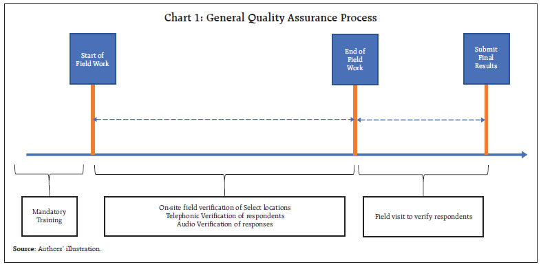

Achieving comprehensive coverage of survey locations for field verification within strict timelines is a challenging exercise involving visiting an adequate number of locations, adhering to survey design specifications, and maintaining the quality of responses. The complexity is heightened when multiple surveys are conducted concurrently across vast areas.

In terms of the survey process, data collection process has rapidly changed in recent years with the advancement and incorporation of information technology. The earlier pen-and-paper interview (PAPI) based data collection methods have been replaced by CAPI by many institutions, which has reduced data collection efforts as well as helped in improving the data quality (Baker et. al., 1995; Couper, 2000; Caeyers et. al., 2010). As a by-product, CAPI also provides respondents’ locational information and time stamps of responses, which are valuable data for analysis and monitoring purposes. The next section presents specific statistical methods designed to leverage this information effectively for off-site monitoring and on-course correction, if necessary.

III. Off-site Monitoring System for Surveys (OMOSYS)

The geographical information can be utilised for selecting locations for field visits. Instead of relying on a purely randomisation approach, the identification of doubtful locations/cases could be facilitated through off-site monitoring system. These identified locations can then be verified physically during subsequent field visits resulting in more targeted monitoring with higher efficiency in terms of time and resource requirements. The OMOSYS was developed with this objective in mind and comprises the following two integral components:

1. Locational measures, which are measures based on location data and

2. Indicator framework for identifying doubtful cases using locational measures.

The methodology for each of the above components is detailed in the following sub-sections.

III.1 Locational Measures

The map of survey location superimposed by respondents’ latitude and longitude serves as a useful preliminary exploratory tool to assess whether an adequate spread and compliance with instructions have been achieved (Chart 2).¹ This raw approach, however, is fraught with logistical inconvenience of regularly preparing and monitoring hundreds of maps, and it offers limited insights into the selection of locations/respondents for field investigation. Accordingly, for effective monitoring, information contained in a map is transformed into statistical measures as detailed below:

Location Distance Gap (LDG)

Considering the primary goal of verification of investigators’ field visit to intended location, the distance of respondents from the intended survey location is considered as a suitable measure, which is termed as LDG. Denoting the latitude and longitude

Equation (1) represents the equirectangular approximation formula for computing spatial distances, particularly efficient for small distances (Silva et. al., 2014). Using this formula, the LDGs can be computed for all respondents from a location. The larger the LDG, the higher is the probability that the survey of corresponding respondent was not conducted at the intended location.

Calculation of LDG measure requires prior knowledge of geo-coordinates of the intended survey location which may not always be readily available. For example, in Indian context, for rural surveys the sampling frame would generally comprise villages, the centroid of village boundary provided by official agencies, available in public domain, can serve as a proxy for location of the village.³ In contrast, addressing this issue for urban surveys is more complex if they rely on the sampling frames based on polling booths or wards, where the boundary details are not readily available in public domain. In the absence of a direct proxy for the locational information of the selected urban survey locations, geo-coding feature provided by various service providers can be utilised to obtain their latitude and longitude.⁴

Respondent Distance Gap (RDG)

In this manner, the RDG for all respondents at a location can be computed. It is important to note that the computations should be carried out for all respondents covered on a single day as the starting point on subsequent day at the same location may not tally with the previous day end location. High RDG values indicate large deviations, while small RDG values suggest a close cluster of observations or respondents. Both scenarios are undesirable when aiming for a uniform spread of respondents within a survey location.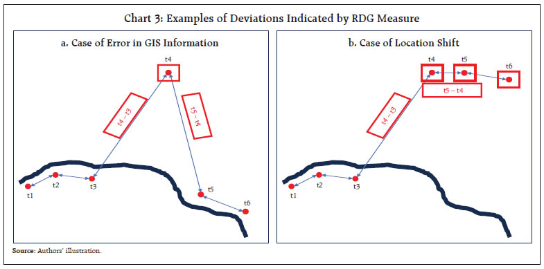

While RDG serves as a useful measure for monitoring, it needs to be acknowledged that at times, in places with weaker internet connectivity, the GPS feature may capture inaccurate locational data especially in remote areas. This may result in computing large distance between successive interviews that do not accurately reflect the actual situation, thereby diluting the effectiveness of analysis by generating false flags. At the same time, since it is known that the locational information may contain errors, there are chances that the true positive signals about instruction violation being overlooked as false positives. As illustrated in Chart 3a, the fourth observation significantly deviates from others, and in Chart 3b, the fourth, fifth and sixth observations, although clustered, deviate from the other cluster of observations. From the RDG measure, it is not immediately apparent whether these deviations are genuine.

Respondent Time Gap (RTG)

To mitigate the challenges associated with interpreting RDG as discussed earlier, the time stamps of the interview commencement, and completion, captured in the CAPI instrument, are found to be extremely beneficial. It is important to note that as long as the investigator uses the same mode of conveyance throughout the day (e.g., walking, cycle, scooter, motorbike), the time needed to cover a specific distance is unlikely to vary significantly. Leveraging on this assumption, the difference between the end time of one interview and the start time of subsequent interview is computed and represented as RTG.

Denoting the start time and end time of interview for the first respondent as (ts_r1,te_r1) and the next respondent, i.e., the second respondent as (ts_r2,te_r2), the RTG for the second respondent can be computed as:

In this way, the RTG for all respondents covered at a location on the same day may be computed. If the RTG for a case flagged by the RDG measure, aligns with the RTG of non-flagged cases at the same location, it may be inferred that the high RDG is likely to be a false positive and could be generated due to signal disruptions. It is important to note that the false positives resulting from signal issues may occur in at least a pair. It is illustrated in Chart 3a where for both 4th and 5th respondent, the distance with the previous respondent is large mainly due to issue with locational information of the 4th respondent. On the other hand, if a high RDG is accompanied by a high RTG, it suggests that the investigator may have deviated from targeted sampling unit/s.

III.2 Indicator Framework

There are two possible approaches to monitor field work using the measures discussed in the previous sub-section depending on the complexity of design and logistics considerations, viz., 1) location-first approach, and 2) respondent-first approach. The location-first approach involves identifying doubtful locations first and then checking respondent data for those locations. In this approach, areas exhibiting a significantly elevated average LDG and both substantially high and low RDG are flagged for further examination. The individual LDG and RDG values of respondents in these identified locations are scrutinised along with their RTG values to avoid false flags. The locations/respondents flagged out of this process may be selected for field visits. The second approach, i.e., the respondent-first approach entails identifying doubtful cases within respondent data and determining the locations with a high number of such cases. The doubtful cases in this approach may require looking at respondent level data directly.

Although both approaches are useful for off-site monitoring, the location-first approach may be employed when number of FSUs are large and within each FSU, a smaller number of responses are obtained. On the other hand, the respondent-first approach may be employed when large number of responses are received from limited number of locations.

When compared to random selection of location/ respondents for field verifications, the locational measures-based approach offers greater advantages as it allows for the off-site selection of doubtful cases. Moreover, while random selection approach only checks a fraction of locations, the proposed method monitors all locations, thereby enhancing the effectiveness and reach of control measures for entire survey data.

In case of small-scale surveys or when there are sufficient resources, the location-first approach or respondent-first approach for flagging doubtful locations/ cases can be performed manually but it becomes difficult especially when the number of locations is extensive, resources are limited, and timeliness is a binding constraint. Additionally, survey data are transmitted to survey originator, either sequentially or in real-time⁵ (the former is more common), which can be passed through a regular quality assessment process. During ongoing survey fieldwork, early identification of deviations from design and instructions becomes crucial in ensuring data quality of subsequent survey interviews. While the measures discussed above can be easily computed once relevant locational data are available, the identification of doubtful cases through manual process may be challenging due to strict timelines, which can be addressed by implementing a system that identifies doubtful cases without requiring manual intervention. In the OMOSYS, this capability has been integrated using indicator approach, where relevant indicators are designed on the top of locational measures discussed earlier to flag doubtful cases. The approach is detailed below:

Model Driven Indicator (MDI) Approach

If data of similar/same/pilot surveys from past time periods is available, the MDI methodology can be used for flagging doubtful cases where models are built using past data.

For location-first approach, the model for the l^th location can take the following general form:

where,

y_l is the variable of interest for lth location;

β_l is the vector of geographical classifications for lth location;

f is the functional form used to model relation between geographical classifications and y_l; and

ϵ_l represents the residual term in model.

For respondent-first approach, without loss of generality, the above model can be defined based on individual respondent-level characteristics, similar to the location-level characteristics defined above. The choice of model depends on the type of survey. Although linear models are widely used, but any other modelling approach can also be integrated. The β_l ’s depend on uniform clustering of locations; that is, within each set of combinations, the expectation is that locations will be uniform in terms of variable of interest. For example, for rural surveys, the components of β_l may include state, district, population group etc. For urban surveys, these components may be city or ward.

The general form for the model as in (4) can be estimated using past data and can be implemented for a system through which sequentially shared data can be checked for outliers. For this purpose, the estimated ϵ_l’s can be standardised, and the extreme values could be flagged after comparing these standardised values with z_p, where z_p is the critical value of standard normal distribution such that Prob(|Z| > z_p) = p or Prob(Z > z_p) = p, as the case may be. The value of p is the level of significance for testing, which could be determined based on the number of doubtful cases that can be examined given the available resources and time constraints. The identified doubtful cases can be chosen for follow-up field visit, allowing for the verification of ground facts.

Fixed Control Indicator (FCI) Approach

There are situations where past data are not available for a survey (e.g., while launching a completely new survey or expanding the coverage of an existing regular survey), where the MDI approach discussed earlier cannot be directly applied. An alternative approach is to build the model sequentially i.e., as the data arrives in batches, the model can be estimated and used to identify outliers in subsequent batches. Subsequently, the model may be re-estimated with the combined data received up to that point, and this process continues until the estimates stabilise.

In case of a non-regular survey, however, allocating extensive resources for model stabilisation might be unnecessary. A natural approach could be to impose fixed control limits on locational measures, based on the experience of originator of survey in alignment with purpose of survey. In such a situation, the fixed-control lower limit (FCLL) and/or fixed-control upper limit (FCUL) can be imposed on the data. Any survey response outside these limits may be flagged as doubtful, requiring further investigation. Although simple, the approach may result in a substantial number of doubtful cases if overly conservative limits are imposed, or it may overlook genuine doubtful cases if limits imposed are too lenient. Another challenge is the natural clustering of locations, where variables of interest may vary widely across clusters: doubtful cases may be observed only in a few clusters if the same limits are imposed uniformly to all clusters, whereas too many limits would need to be imposed with high manual intervention, if limits are to be imposed cluster-wise.

As such, while MDI and FCI approaches have distinct and non-overlapping use cases, the selection of a particular approach also relies on the purpose, type, and resource availability. The subsequent section delves into the details of these approaches and examines their effectiveness in various situations based on synthetic data.

IV. Use Case: Reserve Bank’s Household Surveys

RBI has been regularly tracking the movements in consumer sentiments on major economic parameters through bi-monthly⁶ urban household surveys viz., inflation expectations survey of households (IESH) and the consumer confidence survey (CCS), initiated in 2005 and 2010, respectively. Their sampling frame in urban areas uses polling booths as the FSU, which are regarded as survey locations from which the SSUs (i.e., generally 15-20 households in each FSU) are selected for obtaining responses. Within selected survey location, after a random start and first successful interview, a fixed number of houses are skipped (sampling interval) following right-hand rule for selecting the next household for interview.

Both these surveys cover 19 cities, each surveying over 400 locations from these cities. Aligned with monetary policy cycle of the RBI, these surveys are conducted at a bi-monthly frequency, with survey fieldwork scheduled for 10 days. As discussed in section II, on-site/follow-up field visits constitute an integral component of the quality assurance framework for these surveys. Due to frequent nature of these surveys and stringent timelines, the extensive geographical coverage of survey locations poses challenges in ensuring data quality under the existing quality assurance framework.

The usefulness of OMOSYS is demonstrated in such scenarios through synthetic data generated using the settings and design, such as skipping 10-12 households after each interview and adhering to right-hand rule, of RBI’s household surveys.⁷ The synthetic data is generated in such a way that it contains the essential characteristics of the survey, incorporating a few instances of concern for illustration. Data for locations is generated by using observed average and variances in LDG, RDG and RTG across various states, districts, and population group combinations. For the purpose of illustration, the value of the radius of Earth required for the computation of LDG and RDG using formulas (1) and (2), respectively, is taken as R = 6371.0 km which is the mean value of the radius of Earth.⁸ The data on the geographical locations of all banking outlets within the Centralised Information System for Banking Infrastructure (CISBI)⁹, maintained by the RBI, has been employed as a proxy for the designated survey locations in the calculation of LDGs.

IV.1 Computing Measures

The measures discussed earlier in Section III are demonstrated here with real data. The following cases have been selected for illustration:

• Case 1: A survey location where the instructions are properly followed and, no false alert occurs due to internet signal issue (Chart 4)

• Case 2: A survey location where the instructions are correctly followed, but some false alerts occur due to internet signal issues (Chart 5)

• Case 3: A survey location where there is a deviation from instructions, signalled by an alert raised by the statistical measures (Chart 6)

For Case 1, the measures are computed and presented in Chart 4. Here, ‘duration’ represents the duration of each interview. It is evident from Chart 4b that no significant deviations are observed and the distance gap (RDG) and Time Gap (RTG) exhibit consistency across respondents, as shown in Chart 4a and Chart 4c. On the other hand, for Case 2, two observations are red flagged using RDG measure (Chart 5a). The circle plot of respondents in Chart 5b indicates that these two observations indeed deviated from the cluster of other observations. However, the RTG for these two observations remains consistent with other RTG observations, as indicated by radius of circle and readings in data table. This suggests that the deviations flagged by RDG may be false positives. It is interesting to note that, as discussed in the methodology section, false positives occur in a pair here.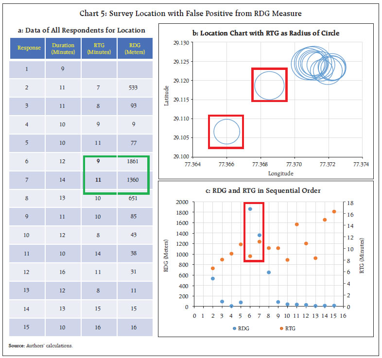

Chart 6 illustrates Case 3, which is distinct from the first two cases. In Chart 6b, two observations visually deviate from the other cluster of observations. The high value of RTG for the first observation, flagged by the RDG measure, implies a high likelihood that the investigator may have moved away from remaining cluster or the intended survey location. The readings of RDG and RTG for subsequent respondent indicate that the investigator, after interviewing the first flagged respondent far away from other respondents, continued to interview subsequent respondents at the same distant location. These respondents are potential cases for field verification.

The above examples have illustrated the capability of locational measures in identifying problematic cases in field surveys through off-site monitoring. Its effectiveness, however, is diluted by the need for manually monitoring of locational measures for all survey locations, which is both laborious and susceptible to errors and omissions. The strategies proposed in Section III.2 to address these limitations are demonstrated below.

IV.2 Flagging Doubtful Cases

Given the sampling design of the RBI’s surveys, which involves a large number of locations with only small number of respondents (generally 15-20) from each location, the more appropriate approach in this context would be the location-first approach, discussed in Section III.2. Thus, the demonstration here will involve the location-first method, i.e., identifying doubtful locations first and subsequently examining survey responses for those locations.

Firstly, we discuss the MDI framework, wherein control limits are derived from synthetic data. For illustration purposes, a linear functional form for model (4) is considered, incorporating geographical classifications such as state, district, and population group. Given the vast geographical and cultural diversity in India, the geographical classifications are important because critical considerations, such as, population density, area dimensions and spread of households are not uniform across states. Even within a state, not all districts are uniform. Since all these factors affect the observed LDG, RDG and RTG, they need to be accommodated in the model to account for variation induced by them in the variables of interest.

Following these settings, the linear location-first models¹⁰ for RDG and LDG for lth location can be written as:

(α₁, β_1i, γ_1j, ξ_1k) and (α₂, β_2i, γ_2j, ξ_2k) are the intercept and fixed effects of state, district, and population group for models (5) and (6) respectively.

ϵ_1ijkl and ϵ_2ijkl represents the residual error term for RDG and LDG models respectively.

For estimation, the synthetic data was split into two parts, the first was used for estimating models (5) and (6), and the second part was treated as fresh data arrival, where estimated model was used to identify doubtful cases. During estimation, the imputed doubtful cases were excluded from dataset to ensure that the model estimates capture only the inherent variations in the survey and is not influenced by extreme observations. The doubtful cases or outliers in the second part of data are identified using the previously discussed standardised estimated residuals methods.¹¹ As discussed in sub-section III.1, both high and low values of RDG are undesirable; thus, a two-sided comparison is used for model (5) with level of significance as p1 = 20 per cent. Whereas for model (6) i.e., LDG, since only higher values are of concern, a one-sided comparison is used with level of significance as p2 = 10 per cent.

The results are presented in Chart 7, where, for clarity, the average RDG and average LDG values are presented in logarithmic terms. The locations identified using the MDI framework are highlighted as red squares. However, a closer examination of these doubtful locations is necessary, specifically, the RDG of each respondent should be scrutinised along with the RTG of these respondents to determine whether a ground visit to the identified location is warranted.

To illustrate the FCI approach, the same dataset is used. For this purpose, the FCLL and FCUL for RDG are considered as 10 meters (log (10) = 1) and 1000 meters (log (1000) = 3), respectively. Similarly, the FCUL for LDG is imposed as 3000 meters (log (3000) = 3.5). The flagged cases are highlighted as green dots in Chart 7. The illustration above indicates that, when limits are properly chosen, both approaches may yield similar results (with a slightly higher number of flags in the FCI approach).

V. Conclusion

In many areas of household surveys, in-person interviews have distinct advantages vis-a-vis telephonic/on-line surveys in terms of obtaining targeted responses, better understanding and much better survey response rate. Good policy decisions and appropriate monitoring require reliable and timely survey data, where ensuring compliance with carefully crafted survey design, especially in geographically extensive surveys, present challenges. Traditional follow-up verification field visits become logistically challenging, especially in remote areas.

The OMOSYS proposed in this article utilises GIS data obtained through CAPI instruments to develop statistical measures for addressing these concerns in a pragmatic manner. It employs locational measures (viz., LDG, RDG and RTG), to identify doubtful cases through off-site monitoring. LDG measures the distance of respondents from the intended location, while RDG and RTG assess compliance with skipping instructions and time gaps between interviews. The system incorporates statistical methods for efficient implementation. The synthetic dataset generated using the settings and design of the Reserve Bank’s household surveys is used to illustrate the effectiveness of OMOSYS. The MDI approach, which uses historical data to set control limits, and FCI approach, which employs fixed limits, are showcased for doubtful case identification. Both the approaches are suited for different survey conditions and the results demonstrate their effectiveness in identifying doubtful cases.

This OMOSYS offers a viable solution for comprehensive survey monitoring, especially in scenarios with limited resources and strict timelines. As against random selection approach, which checks only a fraction of locations, this solution monitors all locations, thereby exponentially enhancing the effectiveness and reach of survey control measures. It ensures a targeted approach to field visits, maximising efficiency and maintaining survey quality across diverse geographical domains. The findings suggest broader applications for improving data quality in CAPI-based surveys across domains.

References:

Baker, R.P., Bradburn, N.M., and Johnson, R.A. (1995). Computer-assisted personal interviewing: An experimental evaluation of data quality and cost. Journal of Official Statistics, Vol. 11, No. 4, 413–431. Retrieved from https://www.scb.se/contentassets/ca21efb41fee47d293bbee5bf7be7fb3/computer-assisted-personal-interviewing-an-experimental-evaluation-of-data-quality-and-cost.pdf

Caeyers, B., Chalmers, N., and Weerdt, J.D. (2010). A comparison of CAPI and PAPI through a randomised field experiment. Retrieved from https://openknowledge.worldbank.org/server/api/core/bitstreams/7aad9cf4-06b4-5332-8ff2-9dc51ec1f016/content

Couper, M.P. (2000). Usability evaluation of computer-assisted survey instruments. Social Science Computer Review, 18(4), 384–396. https://doi.org/10.1177/089443930001800402

Reserve Bank of India. (2009). Report of the Working Group on Surveys, Available at https://rbi.org.in/scripts/PublicationReportDetails.aspx?UrlPage=&ID=557

Reserve Bank of India. (2010). Report of The Technical Advisory Committee on Surveys, Sep-2009. RBI Bulletin, May. Available at https://rbi.org.in/Scripts/BS_ViewBulletin.aspx?Id=11209

Reserve Bank of India (2018). Inflation Expectations Survey of Households: 2017-18. RBI Bulletin October, 105-116, available at https://m.rbi.org.in/Scripts/BS_ViewBulletin.aspx?Id=17820

Reserve Bank of India (2019). The Consumer Rules! Some Recent Survey-based Evidence. RBI Bulletin April, 117-131, available at https://m.rbi.org.in/scripts/BS_ViewBulletin.aspx?Id=18173

Reserve Bank of India. Consumer Confidence Survey, Various Issues, Available at https://www.rbi.org.in/scripts/BimonthlyPublications.aspx?head=Consumer%20Confidence%20Survey%20-%20Bi-monthly

Reserve Bank of India. Inflation Expectation Survey on Households, Various Issues, Available at https://www.rbi.org.in/scripts/BimonthlyPublications.aspx?head=Inflation%20Expectations%20Survey%20of%20Households%20-%20Bi-monthly

Sergey, I.N. (2021). Synthetic Data for Deep Learning. Springer Optimisation and Its Applications. Vol. 174. doi:10.1007/978-3-030-75178-4, https://link.springer.com/book/10.1007/978-3-030-75178-4

Silva, Y.N., Reed, J.M., Tsosie, L.M. and Matti, T.A. (2014). Similarity Join for Big Geographical Data, In E. Pourabbas (Ed.), Geographical Information Systems – Trends and Technologies (pp 20-49), Boca Raton: CRC Press – Taylor & Francis Group. DOI https://doi.org/10.1201/b16871

Survey of India. Online Maps Portal, https://onlinemaps.surveyofindia.gov.in/

Wang D., Li M., Huang X., and Zhang X. (2021). Spacecraft Autonomous Navigation Technologies Based on Multisource Information Fusion. (pp 311) Springer. https://doi.org/10.1007/978-981-15-4879-6

^{^} The authors are Assistant Advisers in New Delhi and Chandigarh Regional Offices, respectively, of the Department of Statistics and Information Management (DSIM), Reserve Bank of India (RBI). They are grateful to Dr. O.P.Mall, Executive Director, Dr. A.R.Joshi, Principal Adviser, DSIM, Shri Ravi Shankar, Adviser, DSIM and the participants of the RBI’s ‘Annual Statistics Conference – 2023’ for their valuable suggestions. The views expressed here are those of the authors, and not of the RBI.

¹ There are many online service providers which provide online maps for different locations. These may be used if maps are not readily available for survey locations.

² The ϕ and λ are in radians. The ϕm must be in units compatible with method used for determining cos(ϕmr).

³ In India, the village boundaries are provided to public by Survey of India which can be accessed at https://onlinemaps.surveyofindia.gov.in/

⁴ For example, Google provides geo-coding services where addresses of location in tabular data may be converted to geo-spatial data.

⁵ Sharing of data from field surveys in real time is very difficult if not impossible due to operational issues (such as inconsistent signal in far flung areas) and cost involved etc. However, for many practical situations, the sequential sharing of data may be sufficient to serve the purpose. The example of sequential data sharing is when data of say all respondents covered on a day is shared as a lot with lag of a day or two.

⁶ Until March 2014, RBI conducted the urban household surveys, namely the ‘Inflation Expectations Survey of Households’ and the ‘Consumer Confidence Survey’, on a quarterly basis. Subsequently, in order to align the surveys with bi-monthly monetary policy framework, two extra rounds (May and November) were introduced.

⁷ Creation of synthetic datasets are useful way of training/testing/illustrating the models in cost and time effective way where the dataset is simulated depicting real life scenarios (Sergey, 2021).

⁸ The mean radius of the Earth is used in this illustration because the Earth is not a perfect sphere; it is an oblate spheroid, meaning it is slightly flattened at the poles and bulging at the equator. The average radius of the Earth takes into account this slight variation in radius due to the Earth’s shape. However, the applicability of formulas (1) and (2) is not confined to this specific choice, and alternative Earth radii, such as equatorial or polar radii (Wang et al., 2021), can be utilized according to specific needs.

⁹ CISBI is the Reserve Bank’s on-line portal for allotment and maintenance of Basic Statistical Return (BSR) codes along with locational details of commercial and co-operative banks as well as other select financial institutions. These cover branches, offices, Non-Administratively Independent Offices (NAIOs), Automated Teller Machines (ATMs), fixed location business correspondents and other fixed location customer service points. The data in tabular form is also made available to public at https://dbie.rbi.org.in/#/banking-outlet

¹⁰ The model may be customised as per the situation and requirements.

¹¹ However, any other outlier detection approach can also be used without loss of generality.