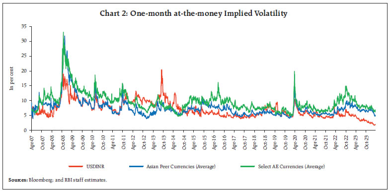
by Saurabh Nath, Dipak R. Chaudhari, Vikram Rajput and Gaurav Tiwari^ This study analyses the trend of India’s Foreign Exchange reserves during major high volatility episodes viz., Global Financial Crisis, Eurozone debt crisis, Taper Tantrum, US-China trade war, the recent Russia-Ukraine conflict and US Fed monetary tightening. It empirically examines major underlying factors impacting the variation in FX reserves such as US Dollar Index (DXY), oil prices, foreign portfolio flows, US financial conditions and market volatility. During the recent Russia-Ukraine conflict and US Fed tightening episode, exchange rate management and reserves faced strong headwinds from trends in DXY, oil prices, foreign portfolio outflows and tight US financial conditions, with the severity of these factors being the highest vis-à-vis the previous high volatility episodes. I. Introduction Foreign exchange (FX) reserves are an instrument to maintain or manage the exchange rate stability, while enabling orderly absorption of international money and capital flows. In India, by statute, the Reserve Bank of India is the custodian of the FX reserves and the reserves are held for precautionary and transaction motives keeping in view the aggregate of national interests, to achieve balance between demand for and supply of foreign currencies, for intervention, and to preserve confidence in the country’s ability to carry out external transactions (Reddy, 2002). In a regime of free float, it could be argued that there is really no need for reserves. If demand for foreign exchange is higher than supply, exchange rates will depreciate and equilibrate demand and supply over time. If supply exceed demand, exchange rates will appreciate and sooner or later, the two will equalise at some price. However, in the light of volatility induced by capital flows and the self-fulfilling expectations that this can generate, as a matter of policy, adequate reserves are required to be maintained (Jalan, 2003). As Emerging Market Economies (EMEs) remain vulnerable to external shocks, a strong umbrella of FX reserves becomes imperative for these countries (Das, 2024). While there is little doubt that FX reserves buffer is of utmost importance during times of volatility, particularly, in the absence of any external support such as Dollar swap lines, the reserves themselves may vary significantly during such episodes. During high volatility episodes, often associated with flight to safety, emerging market currencies face extreme depreciation pressures, impacting their FX reserves. According to the World Bank Treasury’s Reserve Advisory and Management Partnership (RAMP) fourth survey on central banks’ reserve management practices, global foreign exchange reserves dropped 9.3 per cent in 2022, the most significant reserve downturn since 1982. Worldwide reserves shrank by USD 1.4 trillion and were back to pre-pandemic levels. Sixty two per cent out of 156 countries saw a decrease in their reserves, by an average of 12 per cent. Concomitantly, there was a 21 per cent average drop in import coverage, from 6.2 months down to 4.8 months. In addition to interventions to support domestic currencies, valuation also played a role, due to increase in interest rates and cross-currency movements. India’s FX reserves have also witnessed significant dips during high volatility episodes, including during the recent Russia-Ukraine conflict/ Fed monetary tightening episode, which could be due to the Reserve Bank’s FX operations to contain undue exchange rate volatility as well as valuation changes1 in foreign currency assets and gold. In view of the same, this study delves deep into the trend of FX reserves as well as important determinants of FX reserves during the high volatility episodes like Global Financial Crisis, Eurozone Debt Crisis/ Taper Tantrum, EME outflows/US-China Trade war and the most recent Russia-Ukraine conflict/ Fed tightening episode. The study uses an autoregressive distributive lag (ARDL) model to estimate common underlying factors impacting the variation in FX reserves and assesses severity of the factors across crises. The rest of the article has been divided into five sections. Section II covers review of related literature; section III depicts variation in India’s FX reserves in terms of decline from the previous peak and recovery from the trough across the high volatility episodes. Section IV digs into factors underlying the variations in FX reserves during each of the crises. Section V presents empirical estimation, while Section VI concludes with the findings. II. Review of Existing Literature The literature provides diverse views on the factors determining FX reserves as well as motive behind accumulation of reserves. Calvo and Reinhart (2002) observed that emerging economies maintain reserves mainly for managing exchange rate movements rather than managing capital flows. Romero (2005) found that exchange rate volatility and degree of openness are major factors influencing India’s FX reserves while for China, the author could not observe any specific factor. The author noted that increased exposure in the international markets could affect the domestic currency, asset pricing, and even the stock market. Thus, offsetting the effect of an external imbalance on the domestic economy is a powerful motive to hold foreign currency reserves. For example, the Asian Financial Crisis of 1997 started in Indonesia, South Korea and Thailand. Hong Kong, Malaysia, Laos, the Philippines, and China were also affected by the crisis due to their economic ties to these countries. Another incentive to hold reserves is that countries with larger reserve holdings have fared better during financial and currency crises. Dash and Narayanan (2011) found that imports and exchange rate shocks have permanent impact on the reserves. Based on the experience gained during the various crisis episodes, the major objective behind the accumulation of FX reserves, particularly for emerging economies is self-insurance against the volatile capital flows (Jeanne and Rancière, 2011). Steiner (2013) found that central banks accumulate reserves in order to protect the economy from detrimental effects of sudden stops in capital flows and flow reversals. Central banks can use the accumulation of reserves as a substitute for capital controls. Reserves help to manage net capital inflows and permit the central bank to preserve some leeway for an independent monetary and financial policy despite the classic policy trilemma. On the optimum level of reserves, there are various criteria - official reserves to imports, reserves to broad money, and reserves to short-term external debt (Wang and Freeman, 2013). Arslan and Cantú (2019) observe that in early 2000s, the precautionary motive was the main driver of reserves accumulation, while recently, the monetary and exchange rate related goals are playing significant roles. The authors argue that macroprudential policies and swap agreements could alleviate reliance on FX reserve accumulation. Bhasin and Khandelwal (2014) used an autoregressive distributed lag (ARDL) bounds testing approach and found a long-run relationship among exchange rate movements, FII flows and FX reserves in case of India. Raut and Rawat (2022) studying 16 emerging economies found that precautionary motive is the main driver for reserve accumulation as reserves help to reduce the probability of currency crisis. In the case of India, the authors observed that higher FX reserves lower the cost of foreign borrowings. III. Trend of FX Reserves During Various Crises India’s FX reserves have generally trended upwards over time. Since 2007, there has been an accumulation in FX reserves in all years2 barring 5 years, viz., 2008-09, 2011-12 and 2012-13, 2018-19 and 2022-23 (Chart 1). These episodes of reserve depletion have coincided with abnormal global economic and financial developments (Raut and Rawat, 2022).3 In each of the major crises in last two decades4 viz., Global Financial Crisis (GFC), Eurozone Debt Crisis/Taper Tantrum (EZ debt crisis/TT), EME outflows/ US-China Trade war (EME outflows/TW) episode and the most recent Russia-Ukraine war/ Fed tightening (RU/FT) episode, India’s FX reserves have dipped which could be on account of Reserve Bank’s FX operations to contain exchange rate volatility and revaluation of foreign currency assets. However, reserves have stabilised thereafter and resumed their upward trend as headwinds moderated. The Indian Rupee’s implied volatility has witnessed significant jumps during high volatility episodes, mostly in line with major Asian peer as well as advanced economy (AE) currencies. However, the Reserve Bank’s intervention in the forex market and the comfort provided by the large stock of FX reserves, besides various other policy measures, helped contain undue exchange rate volatility and kept FX markets largely stable. Overall, Rupee’s volatility expectations have come down over years as corroborated by trends in implied volatility, risk reversal5 and butterflies6 (Nath et al., 2022). Importantly, the Rupee’s implied volatility remained well below that of major Asian peers7 and select AE currencies8 during the recent RU/FT episode, despite unprecedented headwinds witnessed during the same period (Chart 2). 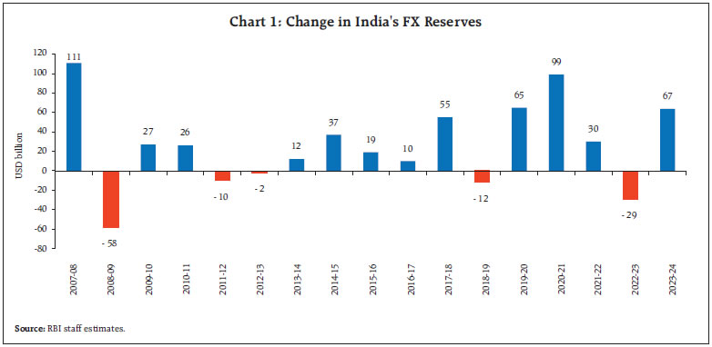
 During GFC, FX reserves dipped to a cycle9 low in just 26 weeks, whereas the recovery took 139 weeks. While the dip in reserves during the EZ debt crisis/ TT was gradual, the recovery was relatively faster. EME outflows/ TW cycle was not only the shortest but the dip in reserves was also the least. During the most recent RU/FT episode, the reserves dipped sharply after remaining steady for the first six months, while recovery took 73 weeks from the cycle low (Chart 3).
The maximum decline in FX reserves in absolute terms was seen during RU/FT episode, at USD 118 billion (peak-to-trough), as compared to USD 34 billion, USD 46 billion and USD 70 billion during EME outflows/ TW, EZ debt crisis/ TT and GFC, respectively (Chart 4). In percentage terms, however, the GFC’s 22 per cent decline in reserves was greater than the 18 per cent dip in RU/FT episode, 8 per cent in EME outflows/ TW and 14 per cent in EZ debt crisis/TT. IV. Factors Underlying Variation in FX Reserves Across Crises The section discusses potential factors which affect Dollar-Rupee exchange rate and FX reserves, viz., US Dollar strength, Crude oil prices, FPI flows, US financial conditions and expected equity market volatility. a) Dollar Index (DXY) and Brent During GFC, the US Dollar Index (DXY) strengthened post onset of the crisis by 23 per cent at its peak, which could have contributed to fall in FX reserves due to a surge in exchange rate volatility and valuation factors (Chart 5.a). However, during the same period, Brent prices plunged by over two-thirds, providing support to the Rupee and FX reserves (via import bill). Over the cycle, average Brent prices were around 63 per cent of prices at the beginning of the crisis. During EZ debt/ TT crisis, DXY strengthened around 11 per cent to its cycle peak, whereas Brent prices oscillated during the episode (Chart 5.b). Similarly, during EME outflows/ TW period, while DXY strengthened by around nine per cent at its peak, Brent prices remained volatile and witnessed sharp fall towards the latter part of the cycle (Chart 5.c). During RU/FT episode, the Rupee and FX reserves faced strong headwinds from both DXY and Brent prices, unlike in the previous high-volatility episodes (Chart 5.d). While DXY strengthened by over 23 per cent at its cycle peak (similar to the GFC), Brent surged by 68 per cent. Though DXY and Brent prices came down from their respective cycle peaks, DXY and Brent averaged 111 per cent and 122 per cent respectively of their beginning of cycle values (as on March 15, 2024), thus, putting a constant pressure on Rupee and FX reserves. In the previous high volatility episodes, the relationship between DXY and Brent has remained negative suggesting that a strengthening Dollar is associated with a decrease in oil prices and vice versa (Chart 6). During the GFC, EZ debt crisis/TT and EME outflows/TW, the correlation between DXY and Brent was (-) 0.76, (-) 0.44 and (-) 0.50 respectively. As oil is priced in US Dollar, a stronger dollar could make oil more expensive for holders of other currencies, thus impacting oil prices. However, during RU/FT episode, the relationship between DXY and Brent turned positive (+ 0.23 correlation). While the DXY surged due to Fed tightening, Brent prices remained elevated due to geo-political tensions, post-Covid supply-chain disruptions and reduction in supply by the OPEC+ members.
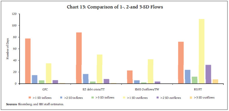
b) FPI Flows Significant portfolio investment outflows happen during periods of heightened volatility mainly due to investors’ flight to safety considerations (Chart 7). i. GFC GFC cycle witnessed large outflows in the initial phase, with cumulative net outflows of around USD 9.5 billion during May 2008 to March 2009 (Charts 8a and 8b). Thereafter, a broad reversal in trend of flows was witnessed and the cumulative net inflows stood at USD 57 billion till July 2011. Further, FPI flows during the GFC episode showed a very high level of Kurtosis (13) or fat tails due to the presence of very high sigma flows viz. an outflow of USD 2.3 billion on September 17, 2008 (a 7-sigma event) and an inflow of USD 2 billion on November 4, 2010 (a 6-sigma event). ii. EZ debt crisis/ TT EZ debt crisis/ TT cycle witnessed lesser quantum of outflows vis-à-vis the GFC with cumulative net negative value of around USD 1.5 billion during September-October 2011 (Charts 9a and 9b). Inflows resumed relatively sooner with cumulative figure rising to around USD 72 billion till July 2014. FPI flows during this period also exhibited fat tails due to high sigma inflows (inflow of USD 2.3 billion on 24 February 2012, a 7-sigma event). On the other hand, no large outflows were observed. iii. EME outflows/ TW EME outflows/ TW cycle witnessed much larger quantum of outflows vis-à-vis GFC and EZ debt/ TT cycle with cumulative net outflows of USD 17 billion during April-October 2018 (Charts 10a and 10b). Thereafter, inflows resumed, leading to net outflows position of USD 1.5 billion till June 2019. Very high sigma FPI inflows (up to 6-sigma) were observed during the latter part of the cycle, though there was absence of very large outflows. iv. RU/ FT RU/FT cycle witnessed largest quantum of outflows compared to all the previous high volatility episodes. Net FPI outflows at their peak rose to as high as USD 36 billion (during September 2021 and July 2022) as against peak cumulative net outflows of USD 9.5 billion, USD 1.5 billion, and USD 17 billion during GFC, EZ debt/ TT and EME outflows/ TW episodes, respectively (Charts 11, 12a and 12b). While strong inflows were witnessed in the latter parts of GFC and EZ debt/ TT cycles resulting in large positive net flow position on a cumulative basis, inflows in the latter part of RU/FT cycle were not as large with net inflow position of $14.5 billion till March 15, 2024. The number of 1-, 2- and 3- standard deviation (SD) outflows during RU/FT cycle was far greater than during other cycles (Chart 13).
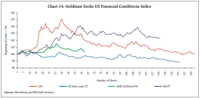
c) Financial Conditions Financial conditions in advanced economies, especially the US, transmit to EMEs through different channels. Many EMEs have current account deficits, which necessarily require net capital inflows from foreign investors. During the most recent high volatility episode, financial conditions in the US tightened due to the US Federal Reserve raising policy rates by 525 bps, US Dollar’s strength, rise in corporate bond spreads and fall in equity prices. Goldman Sachs index of US financial conditions10 remained elevated in the RU/FT cycle with sticky inflation pushing rate cut bets further ahead (Chart 14). There is strong and statistically significant impact of increases in global risk aversion on portfolio flows to emerging markets (Milesi-Ferretti et al., 2011; Broner et al., 2013; Koepke, 2019). The most common proxies for investor risk aversion used in the literature are U.S. implied equity volatility (VIX)11 and the U.S. BBB-rated corporate bond spread over U.S. Treasury securities, which are both found to have a strong contemporaneous impact on portfolio flows. Goel and Papageorgiou (2021) find that lower-rated issuers are more sensitive to changes in global risk appetite as compared to higher-rated issuers. The changing investor base can also play a role, as the exposure of emerging market economies to potentially “flighty” and benchmark-driven investors has been growing (GFSR, October 2019). 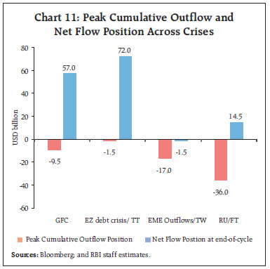 After experiencing crises in the 1990s and early 2000s, many EME central banks accumulated FX reserves to self-insure against large swings in capital flows and exchange rates. This pushed up the average share of FX assets in total assets from 60 per cent in 2000 to over 85 per cent in 2019, which however renders them susceptible to swings in the valuation of foreign assets (Bell et al., 2023). RBI’s balance sheet also saw similar trend with the share of foreign currency assets and gold increasing from 46 per cent in 1999-2000 to 72 per cent in 2022-23. During the recent five years, the share of foreign currency assets (FCA) and gold has remained steady around 72 per cent (Chart 15).12 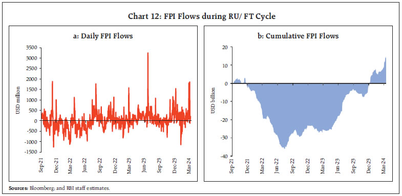
 Due to the surge in global yields, foreign currency assets can also come under extreme pressure on valuation grounds. In comparison to the previous high-volatility episodes where US yields rose only modestly or declined over the crisis, the most recent RU/FT crisis saw average of US 2-year and 10-year treasury yields rising to a level more than six times over the beginning levels and remaining elevated even during the latter part of the cycle (Chart 16). Yields surged globally as most AE and EME central banks embarked on synchronised policy tightening to contain high inflation. d) Expected Equity Market Volatility (CBOE VIX) During RU/FT episode, CBOE VIX witnessed fewer spikes vis-à-vis the GFC and EZ debt/ TT episodes, despite US S&P 500 declining around 19 per cent in 2022, the most since 2008. Further, the equity index recorded 46 moves of 2 per cent in either direction in 2022, the most since 2009, roughly four times the 10-year average of around 11 moves per year.13 Institutional investors are believed to have liquidated equities from their portfolio and shifted to more cash, and thus were left with smaller levels of long-equity exposure in need of hedging. Another reason cited was traders’ increasing reliance on short-term options for tactical trades. The popularity of VIX, which specifically incorporates only options with roughly one month left until expiration, came down with trading in shorter-dated options, including contracts with less than one day left until they expire (zero day to expiry options or 0DTE), surging in popularity. 0DTE contracts accounted for more than 40 per cent of the S&P 500’s total options volume by the third quarter of 2022, almost doubling the percentage from six months earlier.14 Todorov and Vilkov (2024) note trading volume in 0DTEs has risen in recent years because these options are relatively cheap and provide a lottery-like payoff with extremely high, if very unlikely, returns, which appeals to certain investors. Low premiums on 0DTEs allow investors to build in very high leverage, hence the lottery-like payoff profile. Investing in 0DTE options loses money on average, with annualised returns of -32,000 per cent, but on rare occasions generates extremely high returns of up to 79,000 per cent. These returns are much more volatile than the returns on one-month options, which have an average return of -550 per cent annualised and a maximum of 2,500 per cent. 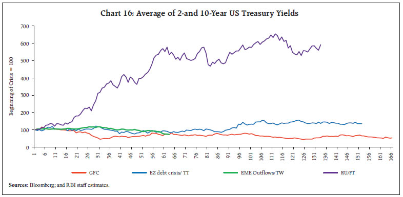 Further, Todorov and Vilkov (2024) suggest an alternative reason behind the compression of VIX: the surge in issuance of yield-enhancing structured products. A simple example of a yield-enhancing structured product is “covered call”: purchase of the S&P 500 index and simultaneous sale of a one-month call option on the index. The product gives an exposure to the index and generates a yield enhancement with the sale of the call option (the premium income), but it gives up part of the upside if the index rises above a threshold. These structured products are frequently offered to retail investors by banks, which are often dealers. The rise of yield-enhancing structured products may dampen volatility due to the mechanics of how dealers hedge option exposures. When dealers sell such structured products, they effectively buy an option from their clients. To hedge the option exposure, dealers buy the equity index when the index goes down and sell when it goes up (dynamic hedging). Thus, dealers act in a contrarian way, effectively dampening the price movements of the underlying equity index. As volatility declines, so does the cost of ensuring against it, as reflected in option prices. 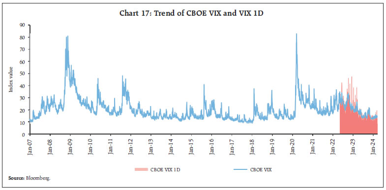 CBOE 1-day volatility index (VIX1D), launched in April 2023, captures the sentiments embodied in 0DTE options and exhibits more spikes vis-à-vis CBOE VIX (Chart 17). V. Empirical Estimation Following the literature (Ramachandran and Srinivasan, 2007; Bhasin and Khandelwal, 2014; Raut and Rawat, 2022), autoregressive distributive lag (ARDL) approach could be appropriate for the modelling of FX reserves dynamics in India. The ARDL model developed by Shin et al. (2014) is suitable for the variables having I(0) or I(1) process as the data contains mix of both (Annex). Further, being a single equation approach, it is suitable to a smaller sample (Chaudhari et al., 2019). Additonally, the derived error correction model (ECM) shows the speed of adjustment needed to restore the long-run equilibrium following a short-run shock (Jena and Sethi, 2021). The select variables and their expected impact (sign) have been presented in the Table 1. Exchange rate deprecation (appreciation) is associated with depletion (accumulation) of FX reserves, thus a negative sign is expected. Similarly, the rise in brent prices and DXY are expected to impact FX reserves negatively. On the other hand, FX reserves are expected to be impacted positively by FPI inflows. A surge in CBOE VIX is expected to exert downward pressure on reserves as uncertainty may lead to safe haven demand at the expense of risk assets. Furthermore, tight US monetary and financial conditions are expected to put downward pressure on FX reserves (in the study, increase in financial conditions index value means tight financial conditions). The ARDL estimation has been applied to all the four high volatility episodes viz., GFC, EZ Debt Crisis/TT, EME outflows/ TW and the most recent RU/FT episode (Table 2). The lag length in the ARDL is based on the adjusted R square process. The long run relationship has been confirmed by the bound test results. USD-INR exchange rate and DXY have statistically significant coefficients with expected signs in all the four episodes. Further, the size of the coefficients increased during the latest high volatility episode (RU/FT) indicating higher impact on the FX reserves. Brent and US financial conditions index are not cointegrated in long run during the GFC episode. Net FPI has positive coefficient across crises indicating outflows on net basis affected reserves adversely, with size of the coefficient being the largest during RU/FT. The US financial conditions index is found to be statistically significant only during the RU/FT episode, which reflects the heightened impact of US monetary policy tightening on the FX reserves during the latest high volatility episode. However, the sign of the VIX coefficient was not on the expected lines, which may be on account of VIX remaining relatively subdued during the RU/FT episode vis-à-vis the previous high volatility episodes for the reasons mentioned elsewhere in the article. Furthermore, statistically significant and negative signs of error correction terms (ECM) are on the expected lines, with the speed of adjustment towards the equilibrium being relatively muted during the EME outflows/TW and the RU/FT episodes. | Table 1: Variables and their Expected Signs | | Variable | Notation used | Expected sign | Source | | FX Reserve | FX | dependent variable | RBI | | USD-INR Exchange Rate | Ex_Rate | - | Bloomberg | | Brent Price | Brent | - | Bloomberg | | Net FPI | FPI | + | Bloomberg | | Volatility Index | VIX | - | CBOE | | GS US Financial Conditions Index | FCX | - | Bloomberg | | Dollar Index | DXY | - | Bloomberg | | Source: Authors’ estimates. |
| Table 2: ARDL Estimation Results | | Variable | GFC | EZ Debt crisis/TT | EME Outflows/ TW | RU/FT | | FX Reserve (-1) | 0.19*** | -0.41*** | -0.60*** | -0.35*** | | | (0.05) | (0.10) | (0.14) | (0.11) | | USD-INR | -0.11** | -0.12*** | -0.23*** | -0.36** | | Exchange Rate | (0.05) | (0.05) | (0.06) | (0.16) | | DXY | -0.59*** | -0.35*** | -0.51*** | -0.89*** | | | (0.05) | (0.07) | (0.10) | (0.11) | | Brent | | 0.08** | 0.03** | -0.04*** | | | | (0.02) | (0.01) | (0.01) | | Net FPI | 0.004* | 0.005** | | 0.01*** | | | (0.002) | (0.001) | | (0.002) | | US Financial | | -0.34 | 0.41 | -2.50*** | | Conditions Index | | (0.67) | (0.68) | (0.01) | | VIX | -0.02*** | -0.01* | -0.02*** | 0.02** | | | (0.01) | (0.01) | (0.01) | (0.01) | | ECM (-1) | -0.17*** | -0.22*** | -0.06*** | -0.02*** | | | (0.03) | (0.04) | (0.01) | (0.004) | | Adjusted R2 | 0.71 | 0.66 | 79 | 70 | | DW | 2.19 | 2.17 | 2.16 | 2.01 | | AIC | -7.47 | -7.99 | -9.57 | -7.74 | | Log-likelihood | 613 | 553 | 236 | 489 | | F-bound test | | | | | | F-stat | 4.001 | 3.48 | 4.57 | 4.11 | | Null: I(0)10 per cent, 5 per cent, 1 per cent, critical values | 1.99, 2.27, 2.88 | 1.99, 2.27, 2.88 | 1.99, 2.27, 2.88 | 1.99, 2.27, 2.88 | | Null: I(1)10 per cent, 5 per cent, 1 per cent, critical values | 2.94, 3.28, 3.99 | 2.94, 3.28, 3.99 | 2.94, 3.28, 3.99 | 2.94, 3.28, 3.99 | | Note: Standard errors are given in parentheses. ***/**/* indicates significant at 1/5/10 per cent level. Lag selection automatic (maximum 12) based on Akaike Information Criterion (AIC). All variables are in log form while net FPI is a dummy variable (assigned 1 for positive values i.e., inflows otherwise 0). | VI. Conclusion While FX reserves have remained under pressure across high volatility episodes viz., Global Financial Crisis, Eurozone debt crisis / Taper Tantrum, EME outflows/ US-China trade war and the recent Russia-Ukraine conflict/ Fed tightening episode, the degree of variation in FX reserves has varied, depending upon the trend of the underlying factors viz., US Dollar Index, oil prices, foreign portfolio flows, US financial conditions and expected equity market volatility. In the case of the recent RU/FT episode, exchange rate management and FX reserves faced strong headwinds from trends in US Dollar Index, oil prices, FPI outflows and tight US financial conditions and the severity of these factors was the highest relative to previous high volatility episodes. However, the Reserve Bank has managed to contain INR volatility and keep FX markets largely stable in all high volatility episodes. Importantly, INR’s implied volatility has remained one of the lowest amongst major Asian peer as well as select AE currencies during RU/FT episode, despite unprecedented headwinds witnessed during this period. Going forward, strength and stability of the Indian economy, its sound macroeconomic fundamentals, financial stability and improvements in India’s external position, particularly the significant moderation in the current account deficit, comfortable foreign exchange reserves and return of capital inflows, are expected to contribute to stability in FX market. References: Arslan, Y., and Cantú, C. (2019). The Size of Foreign Exchange Reserves. BIS Papers, No. 104, 1–23. Bell, S., Chui, M., Gomes, T., Moser-Boehm, P., and Tejada, A. P. (2023). Why Are Central Banks Reporting Losses? Does It Matter?, BIS Bulletin, No. 68. Bank for International Settlements. Bhasin, N., and Khandelwal, V. (2014). Relationship Between Foreign Institutional Investment, Exchange Rate and Foreign Exchange Reserves: The Case of India using ARDL Bounds Testing Approach. International Journal of Finance and Management, 4(2). Broner, F., Didier, T., Erce, A., and Schmukler, S. L. (2013). Gross Capital Flows: Dynamics and Crises. Journal of monetary economics, 60(1), 113-133. Calvo, G. A., and Reinhart, C. M. (2002). Fear of Floating. The Quarterly journal of economics, 117(2), 379-408. Chaudhari, D. R., Dhal, S., and Adki, S. M. (2019). Payment Systems Innovation and Currency Demand In India: Some Applied Perspectives. Reserve Bank of India Occasional Papers, 40(2), 33-63. Das, Shaktikanta (2024). Fundamental Shifts in the Global Economy: New Complexities, Challenges and Policy Options. 59th SEACEN Governors’ Conference. Dash, P., and Narayanan, K. (2011). Determinants of Foreign Exchange Reserves in India: A Multivariate Cointegration Analysis. Indian Economic Review, 83-107. Goel, Rohit, and Papageorgiou, Evan. (2021). Drivers of Emerging Market Bond Flows and Prices. Global Financial Stability Notes No. 2021/04 International Monetary Fund. (2019). Global Financial Stability Report Jalan, Bimal (2003). Exchange Rate Management: An Emerging Consensus? 14th National Assembly of Forex Association of India. Jeanne, O., and Rancière, R. (2011). The Optimal Level of International Reserves for Emerging Market Countries: A New Formula and Some Applications. Economic Journal, 121(555), 905–930. https://doi.org/10.1111/j.1468-0297.2011.02435.x Jena, N. R., and Sethi, N. (2021). Determinants of Foreign Exchange Reserves in Brazil: An Empirical Investigation. Journal of Public Affairs, 21(2), e2216. Koepke, R. (2019). What drives capital flows to emerging markets? A survey of the empirical literature. Journal of Economic Surveys, 33(2), 516-540. Milesi-Ferretti, Gian-Maria, and Cédric Tille. (2011). “The great retrenchment: international capital flows during the global financial crisis.” Economic policy 26, no. 66, 289-346. Nath, S., Rajput, V., and Sankar, G. (2022). Exchange Rate Volatility in Emerging Market Economies. RBI Bulletin, August Ramachandran, M., and Srinivasan, N. (2007). Asymmetric Exchange Rate Intervention and International Reserve Accumulation in India. Economics Letters, 94(2), 259-265. Raut, D. K., and Rawat, D. (2022). Foreign Exchange Reserves Buffer in Emerging Market Economies: Drivers, Motives and Implications. RBI Bulletin, April. Reddy, Y. V. (2002). India’s Foreign Exchange Reserves: Policy, Status and Issues. Economic and Political Weekly, 1906-1914. Romero, A. M. (2005). Comparative Study: Factors that Affect Foreign Currency Reserves in China and India. Honors Projects Papers, 33. Shin, Y., Yu, B., and Greenwood-Nimmo, M. (2014). Modelling asymmetric cointegration and dynamic multipliers in a nonlinear ARDL framework. Festschrift in honour of Peter Schmidt: Econometric methods and applications, 281-314. Steiner, A. (2013). The Accumulation of Foreign Exchange by Central Banks: Fear of Capital Mobility?. Journal of Macroeconomics, 38, 409-427. Todorov, Karamfil, and Vilkov, Grigory (2024). What could explain the recent drop in VIX?. BIS Quarterly Review, March. Wang, Y., and Freeman, D. (2013). The International Financial Crisis and China’ s Foreign Exchange Reserve Management (Issue 49510).
Annex | Table 1A: Stationarity Test (Full Sample) | | Variable | ADF | PP | | t-statistic | Order | t-statistic | Order | | FX Reserve | -10.07*** | I(1) | -26.48*** | I(1) | | Exchange Rate | -21.66*** | I(1) | -25.41*** | I(1) | | Brent Price | -24.73*** | I(1) | -19.60*** | I(1) | | Net FPI | -12.81*** | I(0) | -18.97*** | I(0) | | VIX | -5.24*** | I(0) | -4.95*** | I(0) | | US Financial Conditions Index | -21.53*** | I(1) | -21.53*** | I(1) | | DXY | -5.24*** | I(0) | -4.95*** | I(0) | | Note: ADF: Augmented Dickey-Fuller; PP: Phillips-Perron; ***denote significant level of 1 per cent, while ** denote significant level of 5 per cent. |
| Table 1B: Stationarity Test (GFC Cycle) | | Variable | ADF | PP | | t-statistic | Order | t-statistic | Order | | FX Reserve | -4.58*** | I(1) | -8.99*** | I(1) | | Exchange Rate | -10.14*** | I(1) | -10.06*** | I(1) | | Brent Price | -9.22*** | I(1) | -9.32*** | I(1) | | Net FPI | -5.19*** | I(0) | -9.10*** | I(0) | | VIX | -12.51*** | I(1) | -12.51*** | I(0) | | US Financial Conditions Index | -8.41*** | I(1) | -8.33*** | I(1) | | DXY | -9.17*** | I(1) | -9.17*** | I(1) | | Note: ADF: Augmented Dickey-Fuller; PP: Phillips-Perron; ***denote significant level of 1 per cent, while ** denote significant level of 5 per cent. |
| Table 1C: Stationarity Test (Eurozone Debt Crisis and TT Cycle) | | Variable | ADF | PP | | t-statistic | Order | t-statistic | Order | | FX Reserve | -9.01*** | I(1) | -9.11*** | I(1) | | Exchange Rate | -8.20** | I(1) | -8.14** | I(1) | | Brent Price | -4.37*** | I(0) | -3.20* | I(0) | | Net FPI | -6.55*** | I(0) | -6.53*** | I(0) | | VIX | -3.62*** | I(0) | -3.44** | I(0) | | US Financial Conditions Index | -7.70*** | I(1) | -10.27*** | I(1) | | DXY | -3.76*** | I(0) | -3.82*** | I(0) | | Note: ADF: Augmented Dickey-Fuller; PP: Phillips-Perron; ***denote significant level of 1 per cent, ** denote significant level of 5 per cent, while * denote significant level of 10 per cent. |
| Table 1D: Stationarity Test (EME Outflows/ Trade War Cycle) | | Variable | ADF | PP | | t-statistic | Order | t-statistic | Order | | FX Reserve | -4.29*** | I(1) | -5.74*** | I(1) | | Exchange Rate | -6.40*** | I(1) | -6.40*** | I(1) | | Brent Price | -3.88** | I(0) | -5.36*** | I(1) | | Net FPI | -5.73*** | I(0) | -5.76*** | I(0) | | VIX | -7.47*** | I(1) | -7.79*** | I(1) | | US Financial Conditions Index | -5.81*** | I(1) | -5.58*** | I(1) | | DXY | -3.05** | I(0) | -3.13** | I(0) | | Note: ADF: Augmented Dickey-Fuller; PP: Phillips-Perron; ***denote significant level of 1 per cent, while ** denote significant level of 5 per cent. |
| Table 1E: Stationarity Test (Russia-Ukraine Conflict/ Fed Monetary Tightening Cycle) | | Variable | ADF | PP | | t-statistic | Order | t-statistic | Order | | FX Reserve | -8.01*** | I(1) | -7.85*** | I(1) | | Exchange Rate | -8.01*** | I(1) | -7.85*** | I(1) | | Brent Price | -11.24*** | I(1) | -11.21*** | I(1) | | Net FPI | -5.72*** | I(0) | -5.86*** | I(0) | | VIX | -9.68*** | I(1) | -11.75*** | I(1) | | US Financial Conditions Index | -7.59*** | I(1) | -7.56*** | I(1) | | DXY | -7.95* | I(0) | -7.96*** | I(1) | | Note: ADF: Augmented Dickey-Fuller; PP: Phillips-Perron; ***denote significant level of 1 per cent, ** denote significant level of 5 per cent. while * denote significant level of 10 per cent. |
|