Rigzen Yangdol, Amarendra Acharya and V. Dhanya^*

Received: September 1, 2023
Accepted: November 22, 2023

The paper examines productivity performance of micro, small and medium enterprises (MSMEs) vis-à-vis large firms in India’s organised manufacturing sector in the backdrop of COVID-19. To address simultaneity and endogeneity associated with firm size and productivity, the paper applies the Levinsohn and Petrin method to an unbalanced panel to estimate the production function and calculate the total factor productivity (TFP). The results suggest that productivity levels in financial years 2012 to 2022 were comparable between MSME firms and large firms, with the latter performing marginally better. TFP growth stagnated in the pre-pandemic period for both MSMEs and large firms. Post-COVID-19, productivity increased for both large firms and MSMEs, with productivity growth in MSMEs catching up with that of large firms.

JEL Classification: D2, L6

Keywords: Total factor productivity, Manufacturing firms, COVID-19 pandemic, Levinsohn- Petrin method, MSMEs.

Introduction

MSMEs play an important role in India’s manufacturing sector, accounting for about 45 per cent of the country’s total manufacturing output, 40 per cent of exports, and almost 30 per cent of the national GDP (GoI, 2023a). MSMEs contribute immensely to the socio-economic development of the country by generating employment opportunities and fostering entrepreneurial capabilities among the skilled and unskilled sections of the labour force. Apart from being direct producers, many MSMEs act as ancillary units to large manufacturing firms and produce a wide range of products for both domestic and external markets (ibid). As per National Sample Survey (NSS) 73rd Round, 31 per cent of total MSMEs are engaged in manufacturing sector with more than 50 per cent in the rural sector.

Despite the importance of MSMEs to the economy, their productivity at the firm level has not been analysed specifically. While availability of firm-level data has led to an increase in the studies on firm-level productivity, no distinction is generally made between MSMEs and large firms, mainly due to the absence of data specific to the MSME sector. The change in the definition of MSMEs by the Government of India, which came into effect from July 01, 2020, whereby turnover was included as a criterion for classifying MSME firms. This offers an opportunity to investigate the productivity of MSME sector in detail. As per the new definition, along with investment criterion, firms with a turnover up to ₹5 crore are categorised as micro, up to ₹50 crore as small, and up to ₹250 crore as medium enterprises. Based on this, we have classified MSME firms as those firms having a turnover of upto ₹250 crore, while firms with turnover greater than ₹250 crore are taken as large firms to examine the productivity differential between the two segments, covering the period 2011-12 to 2021-22. We have followed a conservative approach in classifying MSMEs across the time period of study. For example, if a firm has a turnover above ₹250 crore in any year for which data is available, it is categorised as a large firm even if it falls below the limit in some/ remaining years. A similar categorisation for Micro, Small and Medium firms has been followed. MSMEs covered in this paper form part of only the organised manufacturing sector and are not reflective of the entire MSME sector which includes firms in the unorganised sector.

The paper explores the trajectory of TFP in the past decade and studies the effect of COVID-19 by examining the pattern of recovery among MSMEs compared to large firms. Globally, the TFP declined during COVID-19, and India was also no exception (Bloom et al., 2020). As per Conference Board data, India’s TFP witnessed a setback, contracting by 2.8 per cent in 2020, as compared to the global TFP decline of 1.8 per cent. It is widely recognised that MSMEs were severely impacted by the pandemic (Sanobe et al., 2021; and UNICEF, 2021). The pandemic changed many pre-existing patterns of production and demand, affecting the delivery pattern and consumer preferences resulting in loss of front-line customers, and MSMEs’ ability to source raw materials (Schaper and Burgess, 2022).

The MSME sector in India was also severely impacted during the pandemic with supply chain shocks and slowdown in demand - both domestic and external - impacting businesses (Mitra and Gupta, 2021; and Rathore and Khanna, 2021). The Government of India along with the Reserve Bank of India (RBI) brought out a slew of measures to reduce this pandemic-induced stress and revive the sector. The Emergency Credit Line Guarantee Scheme (ECLGS) was brought in to help MSMEs meet their liquidity needs for sustaining business operations, and it played a major part in sustaining credit flow to the MSME sector (RBI, 2023). Apart from these, the registration process was simplified for MSMEs, whereby only permanent account number (PAN) and Aadhaar were made mandatory for the registration. In 2020, the definition of MSMEs was altered to expand the scope and simplify categorisation of MSMEs in the manufacturing and services sectors. Measures undertaken by the RBI included interest rate reduction, infusion of liquidity, debt servicing moratorium, standstill in asset classification, package on loan restructuring, and exemptions in Cash Reserve Ratio (CRR) maintenance on loans to new borrowers. These temporary measures have been particularly effective in supporting firm liquidity (Das, 2021; and Górnicka and Xu, 2021).

Though studies on productivity of the MSME sector are scarce, there exist studies on firm size and productivity, which are applicable to MSMEs. While economies of scale benefit large firms, decreasing returns to managerial efficiency with increase in firm size limit productivity (Williamson, 1967). On the other hand, small firms have greater organisational responsiveness, and they adapt to changes and innovations faster, leading to their improved productivity (Utterback, 1994; and Dhawan, 2001). Our paper adds value to this stream of literature by looking into productivity differentials and performance of MSMEs vis-à-vis large firms.

The paper is organised as follows. The next section gives a review of literature. Section III provides the data and methodology of the study. Section IV presents the results of the estimation of production function, productivity in the MSME sector and large firms, the effect of COVID-19 on average firm-level productivity at the industry-level in MSMEs and large firms, and a disaggregated analysis of productivity in the micro, small and medium sectors. Section V concludes the paper.

Section II
Literature Review

Productivity is considered as a key factor in deciding economic growth of a country in the long run and therefore, it has a major role in improving living standards of people. Difference in productivity is broadly attributed as the reason behind difference in economic performance across countries over time (Krugman, 1997). Productivity gains as reflected by the efficient uses of resources either through new technologies and new ideas or through new ways of production, foster economic growth and channelise limited resources to more productive uses.

The concept of total factor productivity was first introduced in Solow’s seminal paper in 1957. Solow acknowledged that only a part of economic growth was due to increasing capital and labour inputs and that the remainder was caused by technical change. Hence, if inputs in the production function were kept constant, any increase in output was derived from a shift in the way firms produced output (Solow, 1957). Thus, the total factor productivity or the multi-factor productivity is the efficiency of output production. Total factor productivity has the advantage of being invariant to intensity of use of observable factor inputs, unlike the concept of single factor productivity measures like labour productivity, which are impacted by the use of omitted inputs.

Apart from looking at productivity at the aggregate level, macro-economists are also dissecting aggregate productivity growth into various micro-components to better understand the sources of such growth (Syverson, 2011). With the availability of firm-level data coupled with improvements in empirical methodologies, there has been an increase in studies on TFP, both theoretical and empirical (Bartelsman and Doms, 2000). Recent literature has also embarked on explaining aggregate productivity growth via firm-level heterogeneity in productivity (Olley and Pakes, 1996). While aggregate TFP gives a macro perspective, it masks the productivity differences across firms at micro-level. This micro-level picture has policy implications, as detailed information can aid policy makers and financial institutions in resource allocation and can help them gauge competitiveness across firms. Micro data on firm productivity, thus brings a more detailed level of resolution that is not attainable with macro data. It helps to understand sectoral growth drivers, as aggregation of data fails to throw light on the changes in drivers within the economy. This is corroborated by a study on the US productivity during 1995 to 2005, which showed that the TFP surge between 1995 and 2000 was attributed to the IT-producing industries, while it was mostly due to the IT-using industries, many of them in services, during 2001-2005 (Jorgenson et al., 2007).

In the Indian context, there exists a large literature on productivity at the aggregate as well as at the sectoral levels. Studies found a slow or negative growth in TFP in the manufacturing sector during 1951-1979 (Reddy and Rao, 1962; Banerje, 1975; Goldar, 1986; and Ahluwalia, 1985). Post-reform studies are inconclusive about improvement in the TFP growth in Indian manufacturing sector (Balakrishnan and Pushpangadan, 1998; Rao, 1996; Pradhan and Barik, 1998; Trivedi et al., 2011; and Goldar et al., 2017).

Several studies have investigated the relationship between firm size and productivity relying on various indicators of firm size including employment, assets, sales and output. Dhawan (2001), taking assets to identify firm size, found small firms to be more productive than large firms in the US context. On the other hand, a positive relationship was found between firm size and productivity in Canada taking employee number as a proxy for firm size (Leung et al., 2008). Baily et al. (1994) found no significant improvement in productivity for smaller firms when employment was taken as the indicator of firm size. Chen and Lee (2020), looking at productivity slowdown after Global Financial Crisis, found small firms (measured in terms of number of employees) in Europe to have been more adversely affected than their larger counterparts.

In the Indian context as well, there is no definite conclusion on the effect of firm size on productivity. Mazumdar (1991), by taking sales as proxy for firm size, found larger firms to be less productive. Similarly, De and Nagaraj (2014) found that smaller firms, in terms of asset size, having investment in research and better liquidity, are more productive than others. On the other hand, Posti and Maiti (2023) found a positive association between firm size and productivity in the Indian informal sector by taking employee count as the indicator of firm size. While the current paper falls under the larger gamut of literature on firm size and productivity, it uses MSME definition in terms of turnover to differentiate between firm sizes.

Section III
Data and Methodology

The TFP concept has been used to measure productivity or efficiency of conversion of input to output by firms. Since the TFP is not directly observable, it is estimated using the “Solow residual” of the production function. Hence, estimating the TFP requires clarity on the concept and measurement methods, as its correct estimation can guide the policy makers in taking informed decisions (Sampat, 2007).

Traditional methods such as the application of the Ordinary Least Squares (OLS) technique to firm-level give rise to a number of methodological issues. As productivity and input choices seem to be bi-directional in nature, the application of OLS methodology at the firm-level data to derive the production functions can lead to simultaneity or endogeneity problem. A positive correlation between input choices and productivity shocks introduces an upward bias in the estimation of output elasticities for inputs that are freely adjustable (Loecker, 2007). Another problem faced in the estimation of production functions is the selection bias which results when entry / exit of firms is not considered. This causes the productivity estimates to be biased upward as only efficient firms (more likely to survive) are included in the sample. Given this limitation, an unbalanced panel is more representative of the entry and exit dynamics of firms (Altomonte and di Mauro, 2022).

To estimate micro-level TFP, we used four methods: the Ordinary Least Squares (OLS), Fixed effect (FE), Random effect (RE) and the Levinsohn and Petrin (LP) value-added method. The objective behind the application of various methodologies is to explore the sensitivity of productivity measures to variations in methodology and compare parameter estimates derived from each approach for the Indian case. The LP method addresses the endogeneity/ simultaneity in the data set, due to the inherent advantage of the method over traditional methods as has been pointed out in various studies (Bartelsman and Doms, 2000; Biesebroeck, 2007; and Srithanpong, 2016). The Levinsohn and Petrin (2003) methodology improves upon the innovative Olley and Pakes (1996) methodology, which uses micro-level information for correction of simultaneity bias and accounts for self-selection of existing producers. LP method applied to firm-level research, is found to show better estimates of capital output elasticity when applied to an unbalanced panel (Bartelsman and Doms, 2000).

Firm-level analysis faces the problem of heterogeneity where firms reflect differences or variations in the characteristics and behaviour. In the presence of heterogeneity, OLS estimates are not only biased but also inconsistent as the data consists of diverse groups or subpopulations that exhibit different patterns or relationships (Gujarati and Porter, 2008). As stated previously, firm-level panel data is often associated with concerns of endogeneity and simultaneity. Endogeneity occurs where an explanatory variable in a statistical model is influenced by other variables in the model, which can lead to biased and inconsistent estimates of the model parameters. The three main sources of endogeneity have been identified as: omitted variables, simultaneity, and measurement error (Roberts and Whited, 2013). The unobservability of the error term, however, makes it difficult to empirically test whether an endogeneity problem has been solved.

Under the assumption that endogeneity arises from time-invariant omitted variables, the fixed effects estimation can help reduce endogeneity bias, by controlling for time-invariant unobserved factors that may be correlated with both dependent and independent variables. However, if the endogeneity is driven by time-varying omitted variables or measurement errors, fixed effects alone may not be sufficient to address the issue. Likewise, in the random effects model, it is assumed that the unobserved individual-specific effects are not correlated with the explanatory variables. This assumption helps to mitigate endogeneity resulting from time-invariant omitted variables that are correlated with both the explanatory variables and the error term. By including individual-specific effects as fixed effects in the model, the random effects model accounts for these unobserved factors and reduces the bias that may arise from endogeneity. However, the random effects model does not directly address endogeneity arising from time-varying omitted variables or measurement error. If there are endogenous variables that are correlated with the error term or other variables in the model, the random effects model alone may not be sufficient to control for endogeneity.

The simultaneity problem refers to a situation where two or more variables in a statistical model are jointly determined or influence each other simultaneously. It is a specific type of endogeneity that arises when there is a two-way causal relationship between variables. In firm-level productivity analysis, simultaneity can arise when input choices respond to productivity shocks (Levinsohn and Petrin, 2003). In the presence of these issues, not controlling for endogeneity and simultaneity would generate biased estimates of productivity.

Olley and Pakes developed their approach to address the problem of simultaneity, where investment is used to control for correlation between input levels and the unobserved firm-specific productivity processes (Olley and Pakes, 1996). Levinsohn and Petrin used intermediate inputs in place of investments to solve the simultaneity problem (Levinsohn and Petrin, 2003). An advantage of the Levinson and Petrin method over Olley and Pakes is that the intermediate inputs tend to respond to the entire productivity term, whereas investment may be lumpy and not equally responsive. Though the investment proxy accounts for that part of the productivity term to which capital responds, some correlation between the regressors and the error term remains. Intermediate input, on the other hand, generally responds to the entire shock, and hence, is likely to restore consistency.

Even in the presence of measurement errors, studies have found that the semi-parametric methods, like the Levinsohn and Petrin method, for estimating TFP are least sensitive to measurement error, and the correlation between estimated and true productivity remain high (Biesebroeck, 2007). The Levinsohn-Petrin method, thus, addresses the endogeneity problem better by being less prone to measurement errors as well as by addressing issues of simultaneity.

For estimation, we start with assuming a Cobb Douglas production function,

Further, natural log of output and input variables is taken, and the function is transformed as

The resulting equation is,

As these models have methodological issues, as pointed out earlier, we also use the Levinsohn and Petrin (LP) value-added methodology in the estimation of the production function and calculation of productivity. In the value-added method, variable Y is taken after discounting for consumption of intermediate inputs. The LP method has two stages. In the first stage, the Cobb-Douglas production function is assumed with labour as the free variable, capital as the state variable and materials as the intermediate input.

In line with LP method, we use intermediate inputs (here materials) as a proxy for unobserved heterogeneity. On this basis, materials can be written as a function of both the capital and productivity, i.e.,

Rewriting the production function equation as

The first-stage parameters are estimated by using no intercept OLS in this equation. In the second stage, two moment conditions β_m and β_k are identified on the assumption that a) the innovation in productivity ω_it does not influence the capital and b) the innovation in productivity in any period is not correlated with material choice of the previous period¹.

The LP method has faced criticism on account of significant collinearity problems in the first stages of estimation (Ackerberg, Caves, and Frazer, 2006). Additionally, the LP method does not correct for selection bias as it was found that efficiency gains were small when applied to an unbalanced panel (Van Beveren, 2007). Ackerberg, Caves, and Frazer (ACF) (2006) suggested an alternative, where the coefficient of labour is estimated in the second stage along with the coefficients of material and capital. We have incorporated the ACF correction in the LP estimation² and further, used an unbalanced panel to contain selection bias.

Data Description- Coverage and Variable Definitions

Micro-data very often suffers from measurement and data quality issues. The accuracy of TFP growth is heavily dependent on the precision with which the measures of labour and capital inputs are obtained. For our analysis, the financial statements of manufacturing firms were obtained from CMIE Prowess database. We used annual sales as an indicator of output (Y) which were then deflated by industry-specific wholesale price indices. For the construction of labour (L) input, data on total employees, being a non-mandatory disclosure, was not available for most of the companies. Most of the firm-level studies done for India have arrived at labour (L) input by dividing expenditure on wages and salaries by an estimated average total compensation of labour in respective industry, using the data of Central Statistical Office’s Annual Survey of Industries (Balakrishnan and Pushpangadan, 1998; and De and Nagaraj, 2014). However, a comparison of industry-level labour inputs arrived at using this method was found to have large variations with industry-level average employees’ data available in the financial statements of firms in CMIE prowess, with the former resulting in an upward bias for the contribution of labour input.

To overcome this, we took the per unit average compensation of labour for respective industry using CMIE data itself based on those firms which had reported number of employees. A total of 1033 Large companies in our sample had declared the number of employees for at least one year, while 904 companies in the MSME sector had declared number of employees for at least one year. Averaging it across NIC 2-digit classification gave us the divisor factor at NIC 2-digit level, which was used to arrive at the labour component for companies where data on employees were not available.

To elaborate,

Per employee wage, in i^th firm in j^th industry is calculated for firms (i =1 to n), for which data on labour is explicitly obtained from firm financials. For industry code j, (where j = 10 to 32 as per two-digit manufacturing NIC code), per employee wage in i^th firm in j^th industry is calculated as,

We estimate labour employed for firms (b = 1 to n) that do not have data on employees, in industry j using,

For estimating capital (K), the perpetual inventory method was used based on Balakrishnan, Pushpangadan and Babu (2000). For the base year capital stock, gross fixed assets in 2011-12 are adjusted for by deriving the capital at replacement cost from the base year capital, with the use of the revaluation factor³. It was then deflated using price deflators constructed from CSO’s data on gross fixed capital formation to arrive at a measure of capital stock in real terms for the base year. Subsequent years’ deflated investment, GFA_t - GFA_t-1, was added to the existing capital stock at each time-period. For material (M) input, total cost incurred on the purchase of materials and components, including imported raw materials was used. This was deflated using industry-specific material deflator taken from RBI’s KLEMS data. For energy (E) input, data on energy expenses was used from CMIE Prowess, and deflated using industry-specific energy deflator taken from RBI’s KLEMS data.

The estimation approach assumes that the measured productivity levels reflect efficiency of firms. Additionally, we assumed that deflated prices accurately reflect firm’s output and other input variables. An unbalanced panel of 3297 large firms and 3322 MSMEs was taken for the time-period 2011-12 to 2021-22. Summary statistics of the major variables are given in Table 1. Due to presence of outliers, the data was winsorised at 5 per cent on both tails for each variable separately before estimation of production functions.

At the NIC 2-digit level, 23 manufacturing groups were considered (the list is given in Annex A). It was observed that large firms in the sample were concentrated in basic metals, chemicals, machinery and motor vehicles groups. Industries of printing and reproduction of media, wood products and leather products comprised less than 1 per cent each of the total sample, while there was no large firm engaged in furniture manufacturing. MSMEs were concentrated in chemicals, machinery, textiles and basic metals. The industries of printing and reproduction of media, furniture, tobacco products, coke and petroleum and other transport comprised less than 1 per cent of the total MSMEs (Chart 1).

Section IV
Empirical Analysis

Estimation of Production Function

The results of the estimation of production function using four different methods - OLS, FE, RE and the Levinson-Petrin method - are given in Tables 2a and 2b. Energy variable as an input was not used for the LP value added (VA) method as the result was not statistically significant. For the OLS, FE and RE, the same regression was also estimated without energy variable. As estimated parameters were similar, we included energy.

The results indicate that for the Indian manufacturing sector, in the case of both large firms and MSMEs, coefficients of labour, capital, materials and energy are statistically significant⁴. While the Hausman test confirmed presence of endogeneity and found fixed effects methodology to be more suited to the data and analysis, presence of heterogeneity and simultaneity issues warranted the use of the Levinsohn-Petrin method.

Given these considerations, TFP estimated from the Levinsohn-Petrin method has been used. Although the TFP is an analogous concept to labour productivity (which shows output per unit of labour input), in a multi-output multi-input framework, the productivity level is difficult to be measured in any meaningful units. Rather, changes in firm-level productivity over time or movements in firm-level productivity relative to other firms need to be measured with the use of index numbers (Bartelsman and Doms, 2000).

Equation (a) shows change in productivity (π) from period t-1 to period t for firm i; where y represents index of output quantity and x represents index of aggregate inputs.

Equation (b) presents the relative productivity of firm i to that of firm j at a particular time period.

The estimation results suggest that productivity was comparable for large firms and MSME firms, with the former being marginally better across all years; the difference narrowed in 2013-14 and rose marginally thereafter (Chart 2a). The growth in productivity stagnated in large firms till 2014-15 and increased until 2018-19. In 2019-20, productivity dipped sharply in manufacturing. This is in line with the movement in GVA manufacturing, which contracted by 3.0 per cent in 2019-20. Similarly, as per KLEMS data, TFP in manufacturing contracted by 7.8 per cent in 2019-20. For MSMEs, productivity remained near stagnant throughout and dipped in 2019-20. Thereafter, a sharp recovery in productivity growth was recorded for both large firms and MSMEs, with the latter catching up with large firms in terms of growth (Charts 2b and 2c). The recovery in the MSME sector may have been aided by government initiatives like the ECLGS scheme. Lack of bank-firm matched information, however, limits further exploration.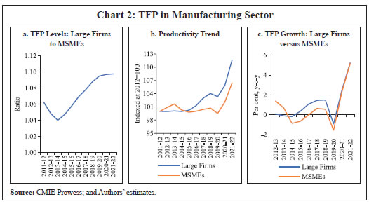

Average TFP levels by NIC 2-digit also suggested that large firms were marginally more productive in most of the sectors, barring in the case of paper and paper products, where MSMEs had higher productivity. As there were no large firms in the ‘furniture manufacturing’, this group was removed. Large corporates in the manufacturing sector were found to be relatively more productive than their MSME counterparts in industries of tobacco, coke and petroleum and food products (Chart 3).

Productivity within the MSME Sector

As the MSME sector is heterogenous, a further analysis of micro, small and medium firms (at the sub-group level of enterprises) was undertaken. In the Indian MSME sector, the micro sub-sector accounts for 99 per cent of the total sector. In our analysis, the micro sector accounts for 45.2 per cent of total firms, small firms account for 51.1 per cent and the remaining 3.7 per cent are medium firms (Chart 4). Productivity at the disaggregated level was also computed using the Levinsohn-Petrin methodology with ACF correction. The production function estimates indicated that coefficients of labour and capital were statistically significant across disaggregated levels, with output elasticity of labour coefficient being higher in micro enterprises, followed by small and medium enterprises. Returns to scale were found to be decreasing across categories (Table 3). Productivity growth stagnated across the sub-sectors in the period before the pandemic. The micro sector’s productivity declined sharply by 2.9 per cent in 2019-20, in line with decline in manufacturing GVA⁵. Post-pandemic, micro enterprises recorded the sharpest recovery in 2021-2022, followed by small and medium enterprises (Chart 5).

Productivity Comparison in Pre- and Post-COVID-19 Period

To study productivity growth in the manufacturing industries in India in the pre- and post-COVID-19 pandemic period for MSMEs and large firms, average⁶ TFP growth from 2012-13 to 2019-20 was compared with average TFP growth during 2020-21 to 2021-22 (Chart 6). In MSMEs, average growth in productivity in the pre-pandemic period was mixed for industries at the 2-digit NIC level. Productivity recorded a contraction in most labour-intensive industries and in transport, machinery and motor vehicles industry. Post-pandemic, productivity increased across industries, with marginal increase observed in printing media and coke and petroleum. Highest productivity gains were recorded in furniture, wood products and paper products (Chart 6a).

For large firms, TFP growth in the pre-COVID-19 period was found to be positive but small (in the range of 0.5 to 1 per cent) for most sectors. The coke and petroleum sector recorded higher productivity growth at 2 per cent, while industries of tobacco production and printed media production recorded a contraction. During 2020-21 to 2021-22, productivity increased across all industries, with the highest growth recorded in paper products, transport equipment and in computers (Chart 6b).

Section V
Summary and Conclusions

The paper uses alternative estimation approaches to estimate firm level production functions for MSMEs and Large Firms in the Indian manufacturing sector for the period 2011-12 to 2021-22. Although MSMEs play an important role in India’s manufacturing sector and contribute immensely to the socio-economic development of the country, productivity literature is sparse at the firm level mainly due to identification issues as previous classifications were based on investment criteria of firms, which were not easily available across firms. The change in the definition of MSMEs by the Government of India in 2020 added turnover as an alternative criterion for classifying MSME firms. Using this classification, this paper investigated productivity of the MSME sector as a whole and in detail viz., micro, small and medium industries.

As per literature, amongst the various techniques of OLS, Fixed effects, Random Effects and Levinsohn–Petrin method, the latter best addresses issues of heterogeneity and simultaneity common in firm-level data. Using this method, total factor productivity was estimated for both MSMEs and large firms. The paper found the organised manufacturing sector in India to be more capital intensive. MSMEs were also found to be marginally less productive on average as compared to large firms. Further, productivity growth stagnated for the sector as a whole, during the pre-pandemic period and dipped sharply in 2019-20. Thereafter, productivity growth recovered with sharper growth recorded in the MSME sector. The growth in productivity in 2020-21 and 2021-22 is in line with recovery in output (value added) in the manufacturing sector, as well as with aggregate sectoral productivity growth in manufacturing as per KLEMS data.

Within industries, in the MSME sector, average productivity growth declined in the period preceding the pandemic across major industries barring some labour-intensive industries and computer manufacturing. In the post-COVID-19 pandemic period (2020-21 and 2021-22), productivity increased across all sectors. For large firms, productivity growth on average, in the pre-pandemic years was marginally positive across most industries. It increased further after the onset of pandemic, with the highest growth recorded in transport equipment and computers.

Within the MSME sector, a disaggregated analysis of production function parameters established micro and small firms to be more labour-intensive. Average productivity growth was muted in the years preceding the pandemic and the dip in productivity 2019-20 was the sharpest for micro enterprises. Post-pandemic, micro enterprises also recorded the sharpest recovery in 2021-2022, followed by the small and medium enterprises. The post-COVID-19 recovery trajectory indicates the resilience and catching up potential in the sector, which may have benefitted from various policy measures undertaken by Government and the RBI.

References

Ackerberg, D., Caves, K., & Frazer, G. (2006). Structural identification of production. MPRA Paper, 38349.

Ahluwalia, I. (1985). Industrial Growth in India, Stagnation since the mid-sixties. New Delhi: Oxford University Press.

Altomonte, C., & di Mauro, F. (2022). The Economics of Firm Productivity. Cambridge University Press.

Baily, M. N., J. Bartelsman, E., & Haltiwanger, J. (1994). Downsizing and Productivity Growth: Myth or Reality?. NBER Working Papers, 4741.

Balakrishnan, P., & Pushpangadan, K. (1998). What Do We Know about Productivity Growth in Indian Industry?. Economic and Political Weekly, 33(33), 2241-2246.

Balakrishnan, P., Pushpangadan, K., & Babu, M. S. (2000). Trade Liberalisation and Productivity Growth in Manufacturing: Evidence from Firm-Level Panel Data. Economic and Political Weekly, 3679-3682.

Banerje, A. (1975). “Capital Intensity and Productivity in Indian Industries. New Delhi: Macmillan.

Bartelsman, E. J., & Doms, M. (2000). Understanding Productivity: Lessons from Longitudinal Microdata. Journal of Economic Literature, XXXVIII, 569-594.

Van Beveren, Ilke. (2007). Total Factor Productivity Estimation: A Practical Review. LICOS Discussion Paper, 182/2007.

Biesebroeck, J. V. (2007). Robustness of Productivity Estimates. The Journal of Industrial Economics. Vol. 55(3), 529-569.

Bloom, N., Bunn, P., Mizen, P., Smietanka, P., & Thwaites, G. (2020). The Impact of COVID-19 on Productivity. NBER Working Paper, 28233.

Chen, S., & Lee, D. (2020). Small and Vulnerable: Small Firm Productivity in the Great Productivity Slowdown. IMF Working Paper, WP/20/294.

Das, S. (2021). Creating New Opportunities for Growth. Address by Shri Shaktikanta Das, Governor, Reserve Bank of India at the Bombay Chamber of Commerce and Industry on February 25, 2021.

De, P. K., & Nagaraj, P. (2014). Productivity and firm size in India. Small Business Economics, 42(4), 891-907.

Dhawan, R. (2001). Firm size and productivity differential: theory and evidence from a panel of US firms. Journal of Economic Behavior & Organization, 44(3), 269-293.

Goldar, B. (1986). Import Substitution, Industrial Concentration and Productivity Growth in Indian Manufacturing. Oxford Bulletin of Economics and Statistics, 8(2), 143-64.

Goldar, B., Krishna, K. L., Aggarwal, S., Das, D. K., Erumban, A. A., & Das, P. C. (2017). Productivity growth in India since the 1980s: the KLEMS approach. Indian Economic Review, Vol. 52, (1), No 3, 37-71.

Górnicka, L., Ogawa , S., & Xu, T. (2021). Corporate Sector Resilience in India in the Wake of the COVID-19 Shock. IMF Working Paper.

Government of India. (2017). Key indicators of unincorported non-agricultural enterprises (excluding construction) in India. Ministry of Statistics and Programme Implementation.

Government of India. (2023). MSME Annual Report 2022-23. Ministry of Micro, Small and Medium Enterprises, GoI.

Government of India. (2023). Union Budget 2022-23, GoI.

Gujarati, D., & Porter, C. (2008). Basic Econometrics (5th ed.). New York: McGraw-Hill Education.

IMF. (2021). Boosting Productivity in the Aftermath of COVID-19. Washington, D.C: International Monetary Fund.

Jorgenson, D. W., Ho, M. S., Samuels, J. D., & Stiroh, K. J. (2007). Industry Origins of the American Productivity Resurgence. Economic Systems Research, 19(3), 229-252.

Kapoor, R. (2018). Understanding the Performance of India’s Manufacturing Sector: Evidence from firm level data. CSE Working Paper, 2018(2).

Kaushik, S. K. (1997). India’s Evolving Economic Model: A Perspective on Economic and Financial Reforms. The American Journal of Economics and Sociology, 69-84.

Krugman, P. (1997). The Age of Diminished Expectations. MIT Press.

Leung, D., Meh, C., & Terajima, Y. (2008). Firm Size and Productivity. Bank of Canada, Working Papers.

Levinsohn, J., & Petrin, A. (2003). Estimating Production Functions Using Inputs to Control for Unobservables. The Review of Economic Studies, 70 (2).

Loecker, J. D. (2007). Product differentiation, multi product firms and estimating the impact of trade liberalisation on productivity, National Bureau of Economic Research. Working Paper 13155.

Mazumdar, D. (1991). Import-Substituting Industrialization and Protection of the Small-Scale: The Indian Experience in the Textile Industry. World Development. Vol.19(1).

Mitra, S., Nikore, M., & Gupta, K. (2021). Enhancing Competitiveness and Productivity of India’s Micro, Small and Medium Enterprises during Pandemic Recovery. ADB Briefs, ADB. doi:DOI: http://dx.doi.org/10.22617/BRF210465-2

Mohan Rao, J. (1996). Manufacturing Productivity Growth: Method and Measurement. Economic and Political Weekly, 31(44), 2927-2936.

Olley, S., & Pakes, A. (1996). The dynamics of productivity in the telecommunications equipment industry. Econometrica, 64, 1263–1297.

Posti, L., & Maiti, A. (2023). Firm Size and Productivity in the Informal Sector: Evidence from India. The Indian Economic Journal.

Pradhan, G., & Barik, K. (1998). Fluctuating Total Factor Productivity growth in Developing Economies: A study of selected industries in India. Economic and Political weekly, 34(12), M92-M97.

Rathore, U., & Khanna, S. (2021). Impact of COVID-19 on MSMEs: Evidence from primary survey in India. Economic and Political Weekly, 56(24), 28-38.

RBI. (2023). Financial Stability Report. June: Reserve Bank of India.

Reddy, M., & Rao, S. (1962). Functional Distribution in the Large Scale Manufacturing Sector in India. Artha Vijnana, 4(3), 189-196.

Roberts, M. R., & Whited, T. M. (2013). Endogeneity In Empirical Corporate Finance 1 Handbook of the Economics of Finance, Vol.2, Elsevier.

Sampat, J. (2007). Total Factor Productivity in Indian Manufacturing: Evidence from a Firm-level Study. Doctoral Dissertation, Emory University.

Schaper, M., & Burgess, R. (2022). The COVID-19 Pandemic Impact on Micro, Small and Medium sized Enterprises:Market Access Challenges and Competition Policy. UNCTAD.

Solow, R. M. (1957). Technical Change and the Aggregate Production Function. The Review of Economics and Statistics, 39, 312-320.

Sonobe, T., Takeda, A., Yoshida, S., & Truong, T. H. (2021). The Impacts of COVID-19 Pandemic on Micro, Small and Medium Enterprises in Asia and their Digitalisation Responses, Vol. 1241. ADB.

Syverson, C. (2011). What Determines Productivity? Journal of Economic Literature, 49(2), 326-65.

UNICEF (2021). Assessing the impacts of COVID-19 on MSMEs in South Asia and East Asia Pacific in Relation to Child Rights. UNICEF ROSA and EAPRO.

Utterback, J. (1994). Mastering the Dynamics of Innovation. Harvard Business School Press, Boston.

Williamson, O. (1967). Hierarchical control and optimum firm size. Journal of Political Economy, 75, 123-138.

Annex A

* Rigzen Yangdol (rigzenyangdol@rbi.org.in), Amarendra Acharya and V. Dhanya work in the Department of Economic and Policy Research (DEPR), Reserve Bank of India. The authors are thankful to Rajib Das, Adviser, DEPR for his guidance and suggestions. The authors also thank Arvind Srivastava, A. K. Shukla, Siddhartha Nath and D. Suganthi for their comments/suggestions. We are also grateful to the participants of 6th Asia KLEMS Conference, Lonavala, June 11-13, 2023, for their valuable comments. The views expressed in the paper are those of the authors and do not necessarily represent those of the institution to which they belong.

¹ For more details on methodology, see Levinsohn and Petrin (2003).

² Prodest module in STATA has been used for LP estimation with ACF correction.

³ For more details on methodology of estimating capital, refer to Balakrishnan, Pushpangadan and Babu (2000).

⁴ The analysis was attempted by inclusion and exclusion of COVID years of 2020-21 and 2021-22. The results showed only marginal changes.

⁵ As per National Account Statistics, manufacturing GVA at constant prices contracted by 3.0 per cent in 2019-20. In 2020-21, a growth of 2.9 per cent was registered.

⁶ While both mean and median TFPs showed similar trends, median TFPs have been used in our analysis to account for heterogeneity in firms.