Sangeetha Mathews^*

Received: January 25, 2023
Accepted: July 6, 2023

This paper harnesses the Artificial Neural Network Quantile Regression model to estimate the systemic risk exposure of select banks in India. The model employs a ‘Leaky ReLU’ activation function to capture non-linearity in risk spillover. The estimated model detects major periods of systemic stress in the last 15 years and suggests that smaller private sector banks are more exposed to systemic risk during stress periods. The estimated model is useful in gauging early signs of rise in systemic risk exposure of individual banks and can complement the micro-prudential risk assessment toolkit of supervisors in initiating timely remedial actions.

JEL Classification: C32, C45, C52, G10, G21, G32

Keywords: Systemic risk, contagion, CoVaR, neural network, quantile regression

Introduction

Financial institutions are interconnected by way of transactions in the form of loans, investments or deposits with one another. Due to such interconnections, a shock striking one financial institution can spread to another institution and can create a ripple effect, ultimately resulting in a systemic failure. Systemic risk refers to such risks, which can lead to a breakdown of the financial system through the channel of contagion. Furfine (2003) cited one more type of systemic risk, “the risk that a financial shock causes a set of markets or institutions to simultaneously fail to function efficiently”.

Systemic risk generally builds up during credit booms or in times of low asset price volatility and materialises during crises. Further, during times of crisis, spillover effects of systemic risk can amplify initial adverse shocks. This ramification of systemic risk was witnessed during the Global Financial Crisis (GFC). Consequently, the Basel Committee on Banking Supervision (BCBS) developed Basel III Standards to improve banking sector’s ability to absorb economic and financial shocks, thereby reducing the risk of spillover from the financial sector to the real economy. These measures taken by the BCBS aided the banking sector worldwide to build sufficient capital and liquidity buffers and is one of the possible reasons for its resilience shown during the COVID-19 pandemic.

The regulatory, monetary and fiscal policies as well as the coordination between these policies are crucial to address systemic risk (Caruana, 2010). Caruana (2010) illustrates the dual dimensions of systemic risk and policy problems concerning each dimension by noting that “the cross-sectional dimension of systemic risk deals with the structure of the financial system, its response to shocks, spillovers and amplification of shocks. On the other hand, the time dimension of systemic risk deals with the build-up of risk over time and its interaction with the macroeconomic cycle. In the former case, the policy problem is how to address the common exposures and interlinkages among financial institutions, while in the latter case, the policy problem is how to address the procyclicality of the financial system and the progressive build-up of financial fragility”.

The assessment of systemic risk and its transmission is, thus, integral to financial stability and policy design, as attempted in this paper. The measurement of systemic risk has gained popularity after the GFC; researchers have developed a multitude of measures to assess systemic risk, the contribution of individual financial institutions to this risk as well as the extent to which a financial institution is exposed to it. Several contagion and systemic risk measures are constructed based on balance sheet-based information or mutual exposures of financial institutions. Numerous indicators have been constructed using stock returns, due to their high frequency nature, data availability without lags as well as the forward-looking behaviour of stock prices in deriving crucial information on systemic risk.

This paper attempts to assess systemic risk exposure of select banks in India. Section II covers a brief literature review on various methodologies used for systemic risk measurement. The methodology for estimating systemic risk exposure of banks in this paper and the concepts behind the methodology are elaborated in Section III. Description of empirical data used in this paper is provided in Section IV. The procedure adopted for training the models used for this study as well as the characteristics of the fitted models are described in Section V, while Section VI discusses the performance of the fitted models. Major results of the study are presented in Section VII and the concluding observations are presented in Section VIII.

Section II
Literature Review

Various methods have been proposed in the literature to measure systemic risk. The “marginal expected shortfall (MES)” proposed by Acharya et al. (2017) is a widely used measure, which estimates “the expected loss of a stock conditional on a crisis”. The “Conditional Value-at-Risk (CoVaR)” proposed by Adrian and Brunnermeier (2011) is another popular measure. CoVaR is defined as the “Value-at-Risk (VaR) of a financial institution conditional on another financial institution being in distress”. The authors employ quantile regressions to estimate CoVaR. The methodology can be applied to estimate the contribution and exposure of a financial institution to systemic risk. Drakos and Kouteras (2013) applied this CoVaR measure to investigate the extent to which various sub-segments of the financial system contribute to overall systemic risk in emerging markets. López-Espinosa et al. (2013) modified the CoVaR methodology by including asymmetries in the specification of Adrian and Brunnermeier (2011).

Meanwhile, Girardi and Ergün (2013) estimated CoVaR using “multivariate GARCH models”, wherein financial distress was defined as “the return of the institution being at most at its VaR”, rather than being exactly at its VaR as proposed by Adrian and Brunnermeier (2011), to allow for more severe distress events. The time-varying correlation of the GARCH model enables not just the systemic risk measurement but also the possible changes over time in the linkage between the bank/financial institution and the financial system. Karimalis and Nomikos (2018) proposed a methodology based on “copula functions” to estimate CoVaR and estimated the systemic risk contribution for a portfolio consisting of large European banks.

Härdle et al. (2016) enhanced the quantile regression based CoVaR methodology by developing a “dynamic Tail-Event Driven Network Model (TENET)” to assess interconnectedness as well as systemic risk in the US financial market. They integrated tail event and network dynamics and proposed “a semi-parametric measure to estimate systemic interconnectedness across financial institutions based on tail-driven spillover effects in a high dimensional framework” and also identified “systemically important institutions conditional to their interconnectedness structure”. Kelibar and Wang (2022) refurbished CoVaR using Artificial Neural Network Quantile Regression model.

Systemic risk tends to get amplified during periods of stress, and risk spillover during such periods can be non-linear in nature. Artificial neural network (ANN) models are efficient in capturing such non-linearity in risk spillover. This paper attempts to assess systemic risk exposure of select banks in India by estimating CoVaR using ANN-quantile regression (QR) method.

Section III
Methodology

III.1 Value-at-Risk

VaR measures the idiosyncratic risk a bank is exposed to. In other words, it focuses on the risk of an individual bank in isolation. During periods of stress, the risk from one bank can get transmitted to another due to interconnectedness among banks/financial institutions. Large, interconnected banks as well as the smaller ones that are systemic as a herd can generate negative risk spillover effects on others. However, VaR cannot capture such risk spillovers. CoVAR addresses the shortcomings of the VaR measure.

III.2 Conditional Value-at-Risk (CoVaR)

III.3 CoVaR Based on Quantile Regression

The Quantile Regression model developed by Koenker and Bassett (1978) is a robust alternative to ordinary least square models in cases where error distributions are non-Gaussian. It is widely used for modelling quantiles of distributions, and therefore, it is appropriate to model tail distributions. Adrian and Brunnermeier (2011) proposed estimation of CoVaR, based on the following quantile regressions models:

III.4 Artificial Neural Network

It is well-known that during periods of stress, systemic risk tends to be amplified and the nature of risk spillover during such periods differs from normal periods. Further, risk transmission is non-linear in nature. As quantile regression is essentially a linear model, it cannot capture the non-linear dimensions of risk. One of the possible ways to model non-linearity is to harness artificial neural networks.

ANN is a data-driven modelling tool which has an architecture based on the structure and function of a biological neural network. This multi-layer computational network contains an input layer, one or more hidden layers and an output layer, wherein each layer consists of nodes. Each node in a layer is connected to nodes in the next layer. The input layer receives the input signals or real-world data. The main feature of an ANN is the presence of hidden layers. The first hidden layer takes inputs from the input layer, performs certain calculations, and passes on the result to the successive layer. The outputs of each layer form the inputs for the successive layer. The computations in each node of a layer can be expressed as a non-linear function z_i of the nodes in the previous layer in the form,

x_is represent the inputs received from the previous layer, w_is are the weightsassigned and b_k is the bias. Ψ is the activation function, a mathematical function which introduces non-linearity to the network. Sigmoid, hyperbolic tangent function (Tanh), softmax, rectified linear unit (ReLU), leaky rectified linear unit (Leaky ReLU), and exponential linear unit (ELU) are some of the common activation functions used in neural networks.

The neural network is trained to learn the parameter values (weights and bias) through forward and backward propagations. Forward propagation involves receiving inputs through the input layer, propagating to the hidden layers, and finally generating the output in the output layer. The predicted output obtained by passing the inputs through the forward network is compared to the target output to calculate a loss or an error function. Backward propagation involves computing the gradient of the loss function and moving backwards from the output to input layer to update the weights of neural network. This iterative procedure of forward and backward propagations is repeated till the loss function is minimised, thereby generating finetuned weights for the neural network. The network structure is determined using a set of variables called hyperparameters. The hyperparameters of an ANN model include the number of neurons in each hidden layer, activation function, optimiser, learning rate, batch size, and epochs. These hyperparameters need to be tuned to get their optimal combination in such a way that the objective function is optimised.

III.5 Artificial Neural Network Quantile Regression

While neural networks are used extensively in classification and linear regression problems, their application in quantile regression is less explored. In linear regression problems, the neural network algorithm generally attempts to minimise the loss function, mean square error (MSE). As quantile regressionmodels quantiles rather than mean, the algorithm attempts to estimate the Ƭ^th conditional quantile by minimising a loss function viz., quantile loss function, defined as,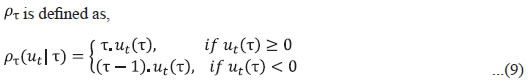

where u_t(Ƭ) = y_t-ŷ_t, Ƭ Ɛ (0,1), y_t and ŷ_t are the actual and estimated values, respectively. The quantile estimator provides much richer information on the whole conditional distribution of y_t and more robust estimates under the presence of outliers and non-linearities as compared to the ordinary least square estimator (Chronopoulos et al., 2021). While quantile regression is essentially a linear model, non-linearity can be introduced in the model by harnessing a neural network to fit the model. This can be achieved by applying appropriate non-linear activation functions in the ANN-QR model.

III.6 Methodology for Estimation of CoVaR Using ANN-QR

In this paper, CoVaR is estimated using ANN-QR model similar to the one proposed by Kelibar and Wang (2022). The relevance of using this approach for estimating CoVaR stems from its flexibility in detecting possible non-linear dependencies in data, as the conditional quantile of a bank/financial institution on another one during times of distress behaves non-linearly. The first step in estimating Artificial Neural Network based CoVaR (ANN-CoVaR)is to estimate VaR. Here, the VaR of the i^th bank is estimated using quantileregression based on a set of macro-financial variables M_t as in equation (3), where the conditional quantile of the error term is zero. VaR is estimated as the fitted value of the quantile regression as indicated in equation (5), such thatthe probability of losses of the i^th bank (Xⁱ_t) less than or equal to VaRⁱ_Ƭ,t is equal to the quantile Ƭ = 95 per cent. Hence, VaR is computed based on the linear quantile approach.

ANN-CoVaR is estimated as a fitted conditional quantile, building on the results of VaR obtained using equation (5). The conditional quantile of bank j’s returns is regressed on the returns of all other banks and a set of macro-financial variables through a neural network as,

Although the approach of Kelibar and Wang (2022) is applied in this paper, there are certain central differences. In this paper, macro-financial variables are also used in the estimation of CoVaR, consistent with the fundamental approach of Adrian and Brunnermeier (2011). Secondly, the Leaky ReLU activation function applied to induce non-linearity in this paper is an improvement over the ReLU activation function used by Kelibar and Wang (2022), as elucidated in Section V.5. In this paper, CoVaRs are estimated for a wider set of 26 banks operating in India, while Kelibar and Wang (2022) analysed eight US Global-systemically important banks (G-SIBs). Kelibar and Wang (2022) used a sliding window for training the data, whereas training is done in batches in this paper.

The methodology for estimating ANN-CoVaR is mainly based on stock prices and it does not consider any balance sheet-based financial performance indicators of financial institutions. Therefore, the efficacy of this methodology depends on market efficiency. Efficient Market Hypothesis (EMH) (Fama, 1970) suggests that when markets are efficient, stock prices of a firm reflect all available information of the firm. If markets are inefficient or less efficient, stock prices need not be reflective of the firm’s performance and in such cases this methodology may not be effective. The methodology is also computationally intensive.

Section IV
Empirical Data

Using the methodology in the previous section, ANN-CoVaR is estimated for a set of 26 listed banks, using the daily stock returns of these banks. For convenience of estimation, the stock returns are converted to losses,Xⁱ_t, defined as,

Thus, stock loss represents the daily percentage loss(+) or gain(-) for an investment in one unit of a stock. As VaR and CoVaR are defined as maximum losses, working with losses rather than returns aids the interpretability of results. VaR and ANN-CoVaR are constructed using stock return losses, Xⁱ_t, as well as M_t, a vector of macro-financial variables. These variables which include daily NIFTY50 returns, yield curve slope, NSE volatility index (VIX) and 10-year BBB bond spread are common risk factors that can have a significant bearing on bank stock returns. The data are extracted from Bloomberg from January 01, 2008 to June 30, 2022.

Section V
Training the ANN-QR Model for Estimating CoVaR

V.1 Train and Test Data

For training the neural network, the data were divided into training and testing samples in the ratio of 70:30, maintaining the time series structure of the data. The model parameter values (weights and bias) for each bank were estimated using the training dataset and the model performance was tested using the test data. The tuning parameters were optimised by choosing the model specification which minimised the quantile loss objective function mentioned by equation (8), using an appropriate optimisation algorithm. The out-of-sample performance of the model was evaluated using the test data.

V.2 Characteristics of the Fitted Neural Network

In this paper, CoVaR was estimated by minimising the quantile loss function for Ƭ = 95 per cent. The neural network for each bank was estimated with one hidden layer (a shallow neural network) for simplicity. However, the number of nodes in the hidden layer, being a hyperparameter, varied from bank to bank due to tuning. For instance, in case of PSB1, a public sector bank (PSB), the optimisation was achieved with ten nodes in the hidden layer. The input layer consisted of 29 nodes representing the stock losses of the rest of the 25 banks as well as the four macro-financial variables, whereas the output layer contained one node representing the final output of the sequential model. The neural network structure of ANN-CoVaR estimated for PSB1 is displayed in Chart 1.

V.3 Batch Size and Epoch

A neural network performs training in batches or sub-samples wherein each batch is passed through the network to learn the parameters. The number of samples passed through the network at a time is called as batch size. Being a hyperparameter, a batch size of 125 was found to be optimal for most of the banks. Therefore, the training was done for most banks in batch sizes of 125, which pertained to almost half year of the data. Training the neural network was done sequentially in disjoint batches using the complete set of training data to complete one epoch. The internal model parameters were updated with completion of each epoch. Epoch was also a hyperparameter and the number of epochs yielding optimal results varied from 16 to 42 for various banks (Annex 1).

V.4 Optimisation Algorithm

The loss function can be minimised using various optimisation algorithms, such as gradient descent, stochastic gradient descent, Adagrad, Adadelta, Adam etc. In this paper, Adam optimiser, an efficient stochastic optimisation algorithm proposed by Kingma and Ba (2014) was applied to optimise the quantile loss function. Adam computes individual adaptive learning rates for different parameters from estimates of first and second moments of the gradients and is well-suited for data with large number of parameters.

V.5 Activation Function

Kelibar and Wang (2022) applied a ReLU activation function defined as max(0,x) for inducing non-linearity. Although ReLU does not suffer from the vanishing gradient or exploding gradient problems which are generally encountered with sigmoid and softmax activation functions, it suffers from a problem known as dying ReLU, which creates certain dead neurons during the optimisation process (Géron, 2022). A ‘Leaky ReLU’ activation function takes care of the disadvantage of the dying ReLU problem by assigning a small weight to negative values. Hence, in this paper, a ‘Leaky ReLU’ activation function was applied to induce non-linearity in the model. ‘Leaky ReLU’ is defined as,

The neural network was modelled using Tensorflow and Keras frameworks in Python software.

Section VI
Model Performance and Robustness

The ANN-QR model for each bank was estimated by minimising the average quantile loss function of the train data set. The out-of-sample performance of the ANN-QR model for each bank was evaluated using average quantile loss of the test data set. Further, the performance of the ANN-QR model of each bank was compared with that of a baseline linear quantile regression (LQR) model estimated at Ƭ = 95 per cent, defined as

A lower value of the average quantile loss of the test data indicates better model performance. A comparison of the average quantile losses of both the models based on the test data sets showed that the ANN-QR model for each bank outperformed the corresponding linear quantile regression model for the bank. This is further substantiated by applying a one-sided Diebold-Mariano (DM) test on the test data sets. The DM test statistic based on the quantile loss differentials between the ANN-QR model and the baseline LQR model results suggested that the ANN-QR model outperformed the corresponding baseline model for all banks, as evident from the p-values (Table 1).

Section VII
Results

Using the methodology illustrated in Section III.6, the systemic risk exposures of 26 banks during the period January 01, 2008 to June 30, 2022 were assessed. The cross-sectional average of the negative returns, fitted VaRs and ANN-CoVaRs of these banks during the sample period are presented in Chart 2. Stress periods were identified based on right tail outliers of ANN-CoVaRs. If the average of ANN-CoVaR for the 26 banks for any day was 1.5 times inter-quartile range above the third quartile (Q3+ 1.5 IQR)¹, it was treated as an outlier. It can be seen that the stress periods identified using this method corresponded with the various episodes of stress affecting the Indian economy. Both VaR and ANN-CoVaR remained elevated during such crisis periods, although the level of ANN-CoVaR was much higher than the corresponding VaR.

In the period considered for this study, the highest peak of ANN-CoVaR was seen at the onset of the first wave of the COVID-19 pandemic (Q1:2020); the second highest was in Q4:2008 during the Global Financial Crisis (GFC). However, the spurt in ANN-CoVaR was more persistent during the GFC period unlike in the pandemic period. Risk spikes could also be observed following the Russia-Ukraine conflict in Q1:2022 and during the second wave of the pandemic in Q1:2021. Other notable spikes were during Q3:2015 at the start of the Asset Quality Review (AQR); Q3:2013 during the taper tantrum; and Q3:2011 during the European debt crisis. This shows that events affecting the stock market, irrespective of whether they originate from within the financial system or outside, can escalate the systemic risk exposure of banks.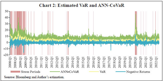

The fitted ANN-CoVaRs can be used to rank banks in the order of their systemic risk exposure during stress periods and non-stress periods. The tail distributions of the fitted ANN-CoVaRs were analysed to identify banks that were more vulnerable to systemic risk (Chart 3). At the median level, ANN-CoVaRs did not vary much across bank groups. However, towards the tail of the distribution, ANN-CoVaRs of private sector banks (PVBs) outweighed those of PSBs. This indicated that in general, PVBs were more susceptible to systemic risk exposure during stress periods.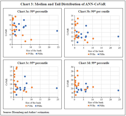

A possible reason for this might be the higher dependence of PVBs’ equity capital on foreign investment inflows, which are susceptible to sudden shocks, by virtue of higher caps² allotted to PVBs as compared to PSBs. Further, PVBs are net borrowers from the financial system and about 74 per cent of the fund-based interbank market is short-term in nature (RBI, 2022). During periods of higher systemic stress, the borrower banks can be exposed to increased rollover risk and liquidity risk, hence can be more impacted by systemic risk than their counterparts. Also, ANN-CoVaR was higher for smaller banks than the bigger ones. Further, ANN-CoVaR of a bank on a stress day was manifold than that on a tranquil day.

During stress periods, tail events tend to spill across banks/financial institutions accentuating systemic risk. However, high systemic risk results in bank insolvency only if such risk materialises. Strong capital and liquidity buffers of banks as well as timely central bank intervention can prevent such risk events from materialising into bank insolvency. The Indian banking system did not witness any materialisation of systemic risk during the stress periods. Nevertheless, if the systemic risk exposure of a bank increases abruptly and persists for a longer period, it can be a cause of supervisory concern. The ANN-CoVaR measure can be utilised to gauge early indications of a rise in systemic risk exposure of banks. Due to the immediate availability of stock market data, the ANN-CoVaR measure constructed on a daily basis can provide early warning signals of stress. This measure can complement other measures designed to assess the micro-prudential risk of individual banks. Supervisors can utilise this measure for monitoring the movements of systemic risk exposure of banks and assessing the change in the dynamics of their relative systemic risk exposure.

Section VIII
Conclusion

Systemic risk assessment is an integral part of financial stability. While Conditional Value-at-Risk computed using the Linear Quantile Regression model is one of the most popular tools to measure systemic risk, it may not be ideal when risk spillovers are non-linear during stress periods. To tide over this constraint, this paper uses machine learning methods to estimate systemic risk exposure of banks. The paper harnesses the neural network quantile regression model to estimate the ANN-CoVaR of 26 major listed banks and attempts to capture the non-linear dimension of risk spillovers during stress periods by inducing a ‘Leaky ReLU’ activation function in the model. The ANN-CoVaR measure is constructed using the daily stock returns of banks, in view of its high frequency nature and timely availability as well as its efficacy from a forward-looking angle.

The out-of-sample tests proved that the estimated ANN-QR model outperformed the corresponding linear quantile regression model. The results revealed the dynamics of select banks’ exposure to systemic risk during stress and non-stress periods. The stress periods identified in the paper corresponded with the various episodes of stress affecting the Indian economy. To illustrate, the highest peak was seen at the onset of the first wave of the COVID-19 pandemic and the second highest during the GFC. At the median level, the ANN-CoVaR measure did not vary much across bank groups. However, towards the tail of the distribution, the ANN-CoVaR of PVBs outweighed those of PSBs, underlining greater susceptibility of the former to systemic risk exposure during stress periods. Furthermore, in the tail region, the ANN-CoVaR measure is higher for smaller banks than the bigger ones, signifying that smaller banks are more exposed to systemic risk during stress periods.

The persistence of CoVaR at a higher level for an extended duration can be a cause of concern. In the Indian context, strong capital and liquidity buffers of banks as well as timely central bank intervention have till now prevented any systemic risk event from causing bank insolvency. It is crucial for supervisory authorities to monitor the movements in systemic risk exposure of individual banks to initiate appropriate remedial actions to prevent any future materialisation of the systemic risk. The estimated ANN-CoVaR can, thus, effectively complement the micro-prudential risk assessment toolkit of bank supervisors. Going forward, the methodology can also be extended to other listed financial institutions to assess the risk spillovers across the various segments of the Indian financial system.

References

Acharya, V. V., Pedersen, L. H., Philippon, T., & Richardson, M. (2017). Measuring systemic risk. The Review of Financial Studies, 30(1), 2-47. https://doi.org/10.1093/rfs/hhw088

Adrian, T., & Brunnermeier, M. K. (2011). CoVaR. National Bureau of Economic Research Working Paper No. 17454. Caruana, J. (2010b, February 12). Systemic risk: how to deal with it? Retrieved from https://www.bis.org/publ/othp08.htm

Chronopoulos, A. Raftapostolos, G. Kapetanios. (2021). Deep Quantile Regression. King’s Business School, Data Analytics for Finance & Macro Research Centre Working Paper No. 2021/1

Drakos, A. A., & Kouretas, G. P. (2013). Measuring systemic risk in emerging markets using CoVaR. Emerging Markets and the Global Economy: A Handbook, 271-307.

Fama, E. F. (1970). Efficient capital markets: A review of theory and empirical work. The Journal of Finance, 25(2), 383-417.

Foreign Exchange Management (Non-Debt Instruments) Rules, 2019, Part II, Sec. 3(ii).

Furfine, C. H. (2003). Interbank exposures: Quantifying the risk of contagion. Journal of money, credit and banking, 35(1), 111-128. https://doi.org/10.1353/mcb.2003.0004

Girardi, G., & Ergün, A. T. (2013). Systemic risk measurement: Multivariate GARCH estimation of CoVaR. Journal of Banking & Finance, 37(8), 3169-3180.

Harvey, D., Leybourne, S., & Newbold, P. (1997). Testing the equality of prediction mean squared errors. International Journal of forecasting, 13(2), 281-291.

Härdle, W. K., Wang, W., & Yu, L. (2016). Tenet: Tail-event driven network risk. Journal of Econometrics, 192(2), 499-513.

Karimalis, E. N., & Nomikos, N. K. (2018). Measuring systemic risk in the European banking sector: a copula CoVaR approach. The European Journal of Finance, 24(11), 944-975.

Keilbar, G., & Wang, W. (2022). Modelling systemic risk using neural network quantile regression. Empirical Economics, 62(1), 93-118.

Kingma, D. P., & Ba, J. (2014). Adam: A method for stochastic optimization. arXiv:1412.6980. https://doi.org/10.48550/arXiv.1412.6980

Koenker, R., & Bassett Jr, G. (1978). Regression quantiles. Econometrica: Journal of the Econometric Society, 33-50.

López-Espinosa, G., Rubia, A., Valderrama, L., & Antón, M. (2013). Good for one, bad for all: Determinants of individual versus systemic risk. Journal of Financial Stability, 9(3), 287-299.

Géron, A. (2022). Hands-on machine learning with Scikit-Learn, Keras, and TensorFlow (3rd ed.). O’Reilly.

Reserve Bank of India (2022). Financial Stability Report, June 2022.

Annex 1. Number of Epochs

^* Sangeetha Mathews (smathews1@rbi.org.in) is an Assistant Adviser in Financial Stability Department, Reserve Bank of India. The author gratefully acknowledges Sneharthi Gayen and Prem Mohan, Financial Stability Department for their feedback on this paper. The author also expresses heartfelt gratitude to Abhishek Ranjan and an anonymous referee for their invaluable comments on this paper. The author is also thankful to the DRG team for their suggestions on this paper. The views expressed in the paper are solely those of the author and do not represent those of the institution to which she belongs.

¹ A popular method used for right tail outlier detection in machine learning.

² Sectoral caps as per Schedule I of the Foreign Exchange Management (NDI) rules, 2019.