|
9.1. Introduction
Economic time series are generally found to exhibit regular, intra-year seasonal movements around its annual trend path. Such repetitive seasonal variations can result from climatic conditions, production cycle characteristics, seasonal nature of economic activity, festivals, vacation practices, etc. While the seasonal variations occur regularly, yet they may vary in magnitude from year to year. From the policy perspective, information on seasonal factors of an economic variable is useful as it enables the policy maker to differentiate between the seasonal changes and long-run changes in a variable and thereby design appropriate policy responses. An article regarding monthly seasonal factors for selected economic and financial time series of the Indian economy is being regularly published in the RBI Bulletin from 1980 onwards. This article presents the monthly seasonal factors of selected economic/financial time series classified into major five groups, namely,
A. Monetary and Banking Indicators;
B. Wholesale Price Index (WPI);
C. Consumer Price Index for Industrial workers (CPI-IW);
D. Index of Industrial Production (IIP); E. External Trade.
The seasonal factors are being estimated using the X-12 auto-regressive integrated moving average (ARIMA) methodology. X-12 ARIMA is the software for seasonal adjustment developed by the US Census Bureau. It is an enhanced version of the X-11 Variant of the Census Method II seasonal adjustment programme. The procedure makes multiplicative/additive adjustments of a time series and creates an output data set containing the adjusted time series and intermediate calculations.
The main source of these new tools is the extensive set of time series model building facilities built into the programme for fitting the regARIMA models. These are regression models with ARIMA (Autoregressive Integrated Moving Average) errors. More precisely, they are models in which the mean function of the time series (or its lags) is described by a linear combination of regressors, and the covariance structure of the series is that of an ARIMA process. If no regressors are used, indicating that the mean is assumed to be zero, the regARIMA model reduces to an ARIMA model. There are regressors for modeling certain kinds of disruption in the series, or sudden changes in level, whose effects need to be removed from the data before the methodology can adequately estimate seasonal adjustments. The regARIMA-modeling module of X-12-ARIMA was adopted from the regARIMA programme developed by the Time Series Staff of Census Bureau’s Statistical Research Division.
9.2. Methodology
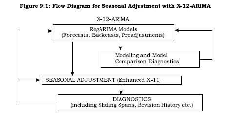
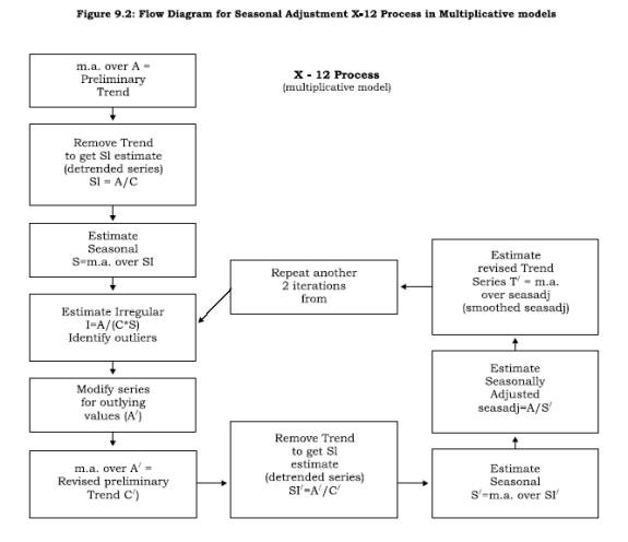
The X-12-ARIMA is developed following the operation-flow diagram of Figure 9.1. This posits a regARIMA (linear regression model with ARIMA time series errors) modeling subprogram that can provide forecasts, backcasts, and prior adjustments for various effects before the seasonal adjustment subprogram in the central box is invoked. The final box in Figure 9.1 represents a set of post-adjustment diagnostic routines that can be used to obtain indicators of the effectiveness of both the modeling and the seasonal adjustment options chosen. The modeling module of X-12-ARIMA is designed for regARIMA model building with seasonal economic time series. To this end, several categories of predefined regression variables are available in X-12-ARIMA (for further details user may refer to the manual available at ‘htttp://www.census.gov/srd/www/ x12a/). User-defined regression variables can also be easily read in and included in models. For a multiplicative model, Figure 9.2 describes X-12 process for computing seasonal factors.
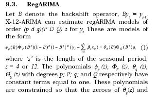
X-12-ARIMA uses the standard
(p d q) (P D Q)s
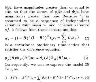
notation for seasonal ARIMA models. The (p d q) refers to the orders of the nonseasonal autoregressive (AR), differencing, and moving average (MA) operators, respectively. The (P D Q)s refers to the seasonal autoregressive, differencing, and moving average orders. The s subscript denotes the seasonal period, e.g., s = 12 for monthly data, or 4 for quarterly data. Great flexibility is allowed in the specification of the ARIMA structures: any number of AR, MA, and differencing operators may be used; missing lags are allowed in AR and MA operators; and AR and MA parameters can be fixed at user-specified values. The specification of a regARIMA model requires specification both of regression variables to be included in the model and also the type of ARIMA model for regression errors (i.e., the orders (p d q) (P D Q)s). Specification of the regression variables depends on user knowledge about the series being modelled.
For the user who wishes to fit customised time series models, X-12-ARIMA provides capabilities for the three modeling stages of identification, estimation, and diagnostic checking. Identification of the ARIMA model for the regression errors follows well-established procedures based on examination of various sample autocorrelation and partial autocorrelation functions produced by X-12-ARIMA. Once a regARIMA model has been specified, X-12-ARIMA will estimate its parameters by maximum likelihood using an iterative generalised least squares (IGLS) algorithm. Diagnostic checking involves estimation of residuals from the fitted model for signs of model inadequacy.
The major improvements in X-12 ARIMA are new modeling capabilities using regARIMA models, sliding spans diagnostic procedure, ability to produce revisions history of a given seasonal adjustment, several new outlier detection options for the irregular component of the seasonal adjustment, etc. RegARIMA is a linear regression model with ARIMA that can provide forecasts and prior adjustments for various effects. X-12 ARIMA uses regARIMA models to preadjust a series by removing effects such as outliers, etc., before the seasonal adjustment program is invoked.
residuals (with standard errors), along with Ljung and Box (1978) summary Q-statistics. X-12-ARIMA can also produce basic descriptive statistics of the residuals and a histogram of the standardised residuals.
An important aspect of diagnostic checking of time series models is outlier detection. The outlier spec of X-12-ARIMA provides the automatic detection of additive outliers (AOs), temporary change outliers (TCs) and level shifts (LSs). X-12-ARIMA’s approach of outliers detection involves computing t-statistics for significance of each outlier type at each time point, searching through these t-statistics for significant outlier(s), and adding the corresponding AO, LS, or TC regression variable(s) to the model.
A seasonal adjustment that leaves detectable residual seasonal and calendar effects in the adjusted series is usually regarded as unsatisfactory. Even if no residual effects are detected, the adjustment will be unsatisfactory if the adjusted values (or important derivative statistics, such as the percent changes from one month to the next) undergo large revisions when they are recalculated as future time series values become available. Frequent, substantial revisions cause data-users to lose confidence in the usefulness of adjusted data. Indeed, such instabilities in the adjustments should cause the producers of adjustments to question their meaning. Unstable adjustments can be the unavoidable result of the presence of highly variable seasonal or trend movements in the series being adjusted. X-12-ARIMA includes two types of stability diagnostics, sliding spans and revision histories.
The sliding spans diagnostics display, and provide summary statistics for, the different outcomes obtained by running the program up to four overlapping subspans of the series. For each month that is common to at least two of the subspans, these diagnostics analyze the difference between the largest and smallest adjustments of the month’s datum obtained from the different spans. They also analyze the largest and smallest estimates of month-to-month changes and of other statistics of interest. They improve upon, or complement in important ways, earlier diagnostics for (i) determining if a series is being adjusted adequately, (ii) for deciding between direct and indirect adjustments of an aggregate series, and (iii) for confirming option
choices such as the length chosen for the seasonal filter or showing that other option choices must be tried.
The second type of stability diagnostic in X-12-ARIMA considers the revisions associated with continuous seasonal adjustment over a period of years. The basic revision calculated by the program is the difference between the earliest adjustment of a month’s datum obtained when that month is the final month in the series and a later adjustment based on all future data available at the time of the diagnostic analysis. Similar revisions are obtained for month-to-month changes, trend estimates, and trend changes. Sets of these revisions, calculated over a consecutive set of time points within the series, are called revisions histories.
9.4. Forecasting
For a given reg ARIMA model with parameters estimated by the X-12-ARIMA programme, the forecast spec will use the model to compute point forecasts, and associated forecast standard errors and prediction intervals. The point forecasts are Minimum Mean Squared Errors (MMSE) linear predictions of future
yt ‘s based on the present
and past
yt ‘s assuming that,
i) the regARIMA model form is correct,
ii) the correct regression variables have been included,
iii) no additive outlier or level shifts will occur in the forecast period,
iv) the specifed ARIMA orders are correct, and
v) the parameter values used (typically estimated parameters) are equal to the true values.
These are standardised assumptions, though obviously unrealistic in practical applications. What is more realistically hoped is that the regARIMA model will be a close enough approximation to the true, unknown model for the results to be approximately valid. Two sets of forecasts errors are produced. One assumes that all parameters are known. The other allows for additional forecast error that comes for estimating the regression parameters, while still assuming that the AR and MA parameters are known.
If the series is transformed, the forecasting results are first obtained in the transformed scale, and then transformed back to the original scale. For example, if one specifies a model of form (1) for yt = log( Yt ), where Yt is the original time series, then yt is forecasted first, and the resulting point forecasts and prediction interval limits are exponentiated to produce point and interval forecasts in the original ( Yt ) scale. The resulting point forecasts are MMSE for yt = log(Yt ), but not for Yt , under the standard assumptions mentioned above. If any prior adjustments are made, these will also be inverted in the process of transforming the point forecasts and prediction interval limits back to the original scale.
If there are any user-defined regression variables in the model, X-12-ARIMA requires that the user supply data for these variables for the forecast period. For the predefined regression variables in X-12-ARIMA, the programme will generate the future values required. If user-defined prior adjustment factors are specified, values for these should also be supplied for the forecast period.
9.5. Limitations
Some of the limitations of X-12-ARIMA procedure are listed below:
1.Observations (data) from a time series to be modeled and / or seasonally adjusted using X-12-ARIMA should be quantitative, as opposed to binary or categorical.
2.Observations must be equally spaced in time, and missing values are not allowed.
3.X-12-ARIMA handles only univariate time series models, i.e., it does not estimate relationships between different time series.
4.The set of automatically identified outliers can change if the regressor set or ARIMA model type is changed.
5.Regressors with t-statistic values just below the critical values can have their t-statistics increase above the critical values as new data are added to the series over time. Conversely, regressors can drop out of the set of identified outliers as new data are added. The printed output of X-12-ARIMA’s automatic-outlier-identification option lists months whose AO or LS regressors are close to the critical values. This is done to enable the user to consider in advance whether to include such regressors in subsequent runs of the program
|