Press Release RBI Working Paper Series No. 06 An Alternative Perspective on Demand and Supply to Forecast Inflation Saurabh Sharma and Ipsita Padhi@ Abstract *Measuring macroeconomic demand and supply is important for a variety of reasons and is especially useful for gauging inflationary pressures. In this context, this paper departs from the standard Blanchard-Quah technique and proposes a novel identification strategy to extricate demand-supply from the business cycle. Based on insights from economy’s production structure and the sectoral output mix, it uses a Bayesian Dynamic Factor Model to obtain two factors that are found to possess relevant characteristics of demand and supply. The gap between the two is found to have a causal relationship with inflation and is a competing predictor of inflation, as compared to other conventional measures of slack such as the output-gap and capacity utilisation. JEL Classification: E3, C38, C67, E37 Keywords: Supply and demand shocks, dynamic factor model, input-output framework, inflation forecast Introduction The concept of demand and supply lies at the very core of economics. Supply refers to the economy’s ability to produce goods and services at given prices, while demand refers to the consumers’ ability or willingness to purchase goods and services at given prices. The dynamic interaction between demand and supply determines the trajectory of output and inflation. Even as this outcome in terms of GDP or inflation is directly observable and measurable (at least approximately), their causal factors (demand-supply) are unobservable and difficult to extricate. The pioneering work in this regard is attributable to Blanchard and Quah (B-Q, 1988), who used a bivariate vector-auto regression (VAR) for real output growth and the unemployment rate to decompose real output into demand and supply disturbances. Their identification was based on the assumption that disturbances with no long-run effect on either output or unemployment are demand disturbances, while those that have no long run effect on unemployment but may have a long-run effect on output, are supply disturbances. This useful economic interpretation of demand-supply disturbances has been used in a number of subsequent studies with further refinements (Spencer, 1996; Enders and Hurn, 2006; Cover et al., 2009). In this paper, we depart from the B-Q methodology and develop a novel framework that incorporates the insights from input-output analysis into a Bayesian Dynamic Factor Model (DFM) to obtain a measure of demand-supply. Obtaining a measure for demand and supply could be important for a variety of reasons. Our focus however lies, almost exclusively, on the inflation-forecasting properties of demand-supply. Any mismatch between demand and supply has implications for the trajectory of inflation. While supply disruptions would pose an upside risk to inflation, demand shortfall is expected to depress inflation. When an economy is simultaneously inflicted with both demand and supply shocks having a potential symmetric/asymmetric impact on inflation, the future trajectory of inflation would be determined by the relative severity of the two shocks. For example, if the impact of demand shortfall outweighs the impact of supply disruptions, inflation would be expected to moderate and vice-versa. Given this consideration, we seek to decompose the business cycle (rather than GDP growth) into demand and supply components1. The business cycle is obtained by applying HP-filter on real GDP to separate the trend and cycle. This decomposition of the business cycle into demand and supply warrants two clarifications. The first pertains to the sources of business cycle fluctuations. While the Neo-Classical school of thought considers that all fluctuations from the trend (determined by supply side factors), i.e., the business cycles are a result of temporary demand shocks, the real business cycle models (Kydland and Prescott, 1982; Long and Plosser, 1983; Prescott, 1986) attribute all fluctuations in output, whether short-run or long-run, to real factors. An amalgamation of these two alternate perspectives was provided in the seminal work of Shapiro and Watson (1988), who used a structural VAR framework to identify the sources of business cycle fluctuations and found that variations in output in the short-term could be caused due to both demand and supply-side factors. Our premise that the business cycle can be decomposed into both supply and demand factors, is based on this finding. We follow their tradition in assuming that the business cycle consists of both demand and supply disturbances. This does not seem unreasonable, especially in the context of a developing country and it is easy to think of several temporary supply disruptions – civil unrest, strikes, disaster, transport disruptions (like the Suez Canal blockage2), monsoon failure, etc. Secondly, since the business cycle, obtained by filtering out the trend, is decomposed into demand-supply in this paper, the estimated demand-supply indices do not capture any long-run supply factors. As mentioned earlier in the paper, this has been done as we are primarily concerned with using the demand-supply indices to forecast inflation in the short-term (a one year horizon). The demand-supply indices estimated in this paper should, therefore, be accordingly interpreted as representing the demand-supply conditions in the short run. The paper proposes a new framework for identifying demand-supply using sectoral outputs3 and input-output linkage measures, with a detailed discussion of why we believe that the indices obtained using our framework would effectively capture demand and supply conditions. After obtaining the demand-supply indices using this framework, we prove that the estimated indices do represent demand and supply in four different ways – (i) The estimated supply is found to be more persistent than estimated demand; (ii) The estimated demand is found to be more volatile than estimated supply; (iii) The estimated indices are in line with the major demand and supply events in the economy like the Global Financial Crisis, the Taper Tantrum, etc.; (iv) A demand-supply mismatch index (constructed simply as estimated demand minus estimated supply) is found to be a competing predictor of inflation vis-a-vis other conventionally used measures of excess demand. Although we devote considerable time to justify that the estimated indices represent demand and supply, through conceptual explanation as well as empirical evidence, it may be stated at the outset that the nomenclature of the two indices is irrelevant for the sake of the inflation analysis. The framework proposed in the paper extracts two indices from sectoral outputs using a DFM framework and input-output linkage measures. The indices, thus estimated, are found to possess important information about inflationary pressures and are useful in forecasting inflation. Thus, a major contribution of the paper is that it presents an alternative framework for forecasting inflation, and this does not rely in any way on the naming of the two indices. The nomenclature becomes important only when we want to understand the mechanism and add an economic interpretation to the econometrics. Against this background, the paper is structured as follows. After a brief review of the literature in section II, we turn to the empirical strategy in section III. Section IV presents the data, and section V sets out the empirical results. Section VI analyses the relationship of the estimated demand and supply indices with CPI inflation, and the last section concludes. II. Literature Identifying demand and supply shocks has always been an important topic in macroeconomic research. The pioneering work in this regard is that of Blanchard and Quah (B-Q), 1988 who used a structural vector autoregression (SVAR) framework to decompose movements in real output growth and unemployment into demand and supply shocks. Their study is based on the interpretation that the shocks which have a temporary effect on output are demand shocks, while those having a permanent effect on output are supply shocks. Further, the aggregate demand and supply shocks are assumed to be uncorrelated. Thereafter, a number of studies have refined the B-Q methodology further by changing the choice of variables used thereby employing identification strategy. For example, Spencer (1996) applied the B-Q identification technique to a bivariate VAR of output and price level. Enders and Hurn (2006) and Cover et al. (2009) modified the B-Q procedure to allow correlation between aggregate demand and aggregate supply. A VAR framework has also been used to decompose inflation into different kinds of shocks in the case of India (RBI, 2020). The interpretation of demand-supply disturbances adopted under the B-Q methodology is subject to several caveats. If there are many supply and demand disturbances, with both permanent and transitory effects on output, and if they all play an equally important role in impacting aggregate level fluctuations, the B-Q decomposition fails. Even when all the supply disturbances have permanent output effects, and all the demand disturbances have only transitory output effects, the B-Q methodology will produce meaningful results only under a set of necessary and sufficient conditions (Blanchard and Quah, 1988). Consequently, we devise an alternate framework for estimating demand and supply based on the dynamic factor model and the input-output literature. Inspired by the seminal work of Stock and Watson, 2010, dynamic factor models have become popular in the economic literature. The premise of a dynamic factor model is that a few latent dynamic factors drive the co-movements of a high-dimensional vector of time-series variables, which is also affected by a vector of idiosyncratic disturbances (Stock and Watson, 2010). DFMs are widely used to extract potential output/output gap from a vector of economic activity indicators (Jarocinski and Lenza, 2015), and to extract the underlying trend inflation from disaggregated data on sectoral inflation (Stock and Watson, 2015). In our case, we use the DFM equation to extract the common unobserved factors of demand and supply from sectoral outputs. Our identification strategy also relies on the input-output literature. Input-output analysis provides the tools to assess structural changes in the economy, in terms of linkages between various economic sectors4. Input-output analysis has been used to study the impact of input shocks on general price level (Berument and Tasci, 2002; Wu et al., 2012), though most of these studies narrowly focus on the inflationary impact of crude-oil prices only. Our methodology differs from these studies as we use the input-output tables to determine the relative extent to which a sector’s output contains information about macroeconomic demand and supply. More precisely, input-output analysis allows us to measure the degree to which a sector demands or supplies inputs. III. Empirical Strategy The objective of this paper is to decompose the business cycle into demand and supply: In order to do this, we adopt a Bayesian DFM framework5. The empirical strategy is explained in four parts: the first sub-section presents the rationale for inclusion of both demand and supply in the business cycle, the second sub-section explains the DFM framework, the third sub-section deals with the determination of the factor loadings in the DFM equation, and the last sub-section presents a conceptual explanation of the mechanism. III.1 Sources of Business Cycle One way of decomposing output that has become commonplace in the literature is the trend-cycle distinction. Statistical filters like the Hodrick-Prescott (HP) filter or the band-pass (BP) filter are often used to filter out the long-term steady component as potential/trend output, and the fluctuation of actual output around this trend is obtained as the business cycle or output gap. This dissection is at the heart of the Neo-Classical synthesis, according to which the potential or “natural” level of output is the long-run equilibrium level that is determined by structural or supply-side factors like the capital stock, labour force, technology, etc. The short-run fluctuations or the business cycles are a result of temporary shocks to aggregate demand. According to this school of thought, the trend and cycle may, therefore, be related to supply and demand, respectively. In contrast, the real business cycle models (Kydland and Prescott, 1982; Long and Plosser, 1983; Prescott, 1986) attribute all fluctuations in output, whether short-run or long-run, to real factors. An amalgamation of these two alternate perspectives was provided in the seminal work of Shapiro and Watson (1988), who used a structural VAR framework to identify the sources of business cycle fluctuations. The key identification criteria used in their analysis was that the long-run level of output is determined by supply shocks6. This assumption allowed for the possibility that short-run fluctuations are largely explained by demand shocks (the Neo-Classical approach), even while it did not exclude the possibility of supply-side shocks affecting short-run output movements (the real business cycle approach). Using quarterly data for the US, they showed that two supply shocks – the productivity and the labour supply shock, accounted for more than 50 per cent of the variations in output, even in the short-term (a two-year horizon). That business cycles may occur due to both demand and supply disturbances was also noted by Blanchard and Quah (1988), who stated that an association of their estimated supply/demand to trend/cycle is unwarranted as supply disturbances can affect not just the trend, but also the business cycle in the presence of price rigidity. The role of supply-side factors in explaining short-run output fluctuations becomes even more important in developing countries. Evidence for developing countries in Asia and Latin America suggests that the main source of output fluctuations in the short-run (and long-run) are supply shocks (Hoffmaister and Roldos, 1997). An analysis of 15 developing countries (including India) shows that supply shocks are often a major source of short-run fluctuations in developing countries (Rand and Tarp, 2002). Thus, it is reasonable to decompose the business cycle into demand and supply. III.2 The DFM Framework While the demand and supply in the economy are not directly visible, their dynamic interaction manifests in the form of final output are observable and measurable. Accordingly, we posit that sectoral outputs7 can contain useful information about aggregate demand and supply, which may be extracted using a Bayesian dynamic factor model. A dynamic factor model can be used to draw out unobserved common dynamics from a vector of observed time series (Stock and Watson, 2010). Ergo, we set up a framework in which two factors, that represent causal demand and causal supply, can be extracted by adopting the following specification:  Based on these considerations, we derive the factor loadings using the economy’s input-output tables, which is explained in the next section. As we will see, the extent to which a sectoral output contains information about demand (c1) is determined by its backward linkages, while the degree of information it possesses about supply (c2) is determined by its forward linkages. These factor loadings are exogenously imposed on this DFM specification to extract the unobservable causal factors – demand and supply. III.3 Determination of factor loadings The economy is composed of multiple sectors, wherein each sector relies on the flow of inputs from other sectors to produce their own output which, in turn, is routed towards other downstream sectors (Chart 1). Looking in this way, the economy is nothing but an intricate production network which works behind the screen to generate final output. The importance of this production network can be gauged by the fact8 that the total value of input flows across sectors is of the same order of magnitude as aggregate GDP itself. 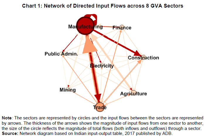 This production structure of the economy is captured by the input-output tables, which show the linkages (input-output relationship) between the various sectors. There are two kinds of economic linkages: backward linkage and forward linkage. Consider a particular sector, i. An increase in output of sector i would result in increased demand for the products which are used as inputs in sector i. This demand relationship is referred as backward linkage. Simultaneously, the increase in output of sector i would increase the availability of inputs to those sectors which use i as an input in their production process9. This supply relationship is termed as forward linkage (Miller and Blair, 1985, 2009; Guo and Planting, 2000; Reis and Rua, 2009). Thus, an increase in production in the sectors which have more forward linkages (e.g. agriculture) provides a kind of supply boost to the economy, while an increase in production in the sectors which have more backward linkages (e.g. textiles) provides a kind of demand boost to the economy. This forms the basis of our identification strategy and we posit that the amount of information contained about demand and supply in a given sectoral output is determined by its backward linkages and forward linkages, respectively. Accordingly, we reframe our DFM equation as follows:  Along the lines of Chenery and Watanabe (1958)10, backward linkages (BLi) have been defined11 as the amount of intermediate inputs sourced from the same as well as other sectors to produce one unit of output of sector i. Similarly, the forward linkages (FLi) are defined as the fraction of the output of sector i that is used as an input in the same as well as other sectors. The degree of forward and backward linkages differs across the sectors (Chart 2 and 3). Some sectors show a higher degree of forward linkage than backward linkage, while opposite holds for other sectors. In the former case, any increase in production in these sectors would boost input-availability to a number of sectors, representing a supply-side effect. This satisfies the first criterion. Also, some sectors are more linked with other sectors while some are less linked. If a sector is less linked, then it has less information about both demand and supply – this fulfils the second criterion. III.4 Explanation of the Mechanism The last sub-section claimed that the factor loadings can be determined on the basis of the linkage measures. In this sub-section, we undertake a detailed explanation of the rationale for the same. First of all, it may be stated that our interpretation of a disturbance as demand or supply is based on the overall impact of the shock on the economy, rather than the initial nature of the shock. For example, a production boost is usually considered a supply shock, but its actual impact on the economy may be demand inducing (if the sector experiencing the production boost has more backward linkages) or supply inducing (sector with more forward linkages). This is imperative since we want to use the estimated indices for inflation forecasting. To make this point clearer, we shall take a few specific examples. Consider two schemes in the textiles sector - the Production Linked Incentive (PLI) scheme12 which is a supply-side intervention and the export promotion scheme that is a demand-side intervention. How will the proposed framework distinguish between these two effects? Since both the schemes increase production in the same sector, our framework will not be able to distinguish between the two shocks. This is, however, not a limitation of the model. If we want to gauge the inflationary impact of a shock, then the initial nature of the shock does not matter much. Now consider the following line of argument: the PLI scheme is expected to boost the supply of textiles (and therefore depress inflationary pressures in the textiles sector) and the export-promotion scheme is expected to create a demand for textiles (and therefore create inflationary pressures in the textiles sector). Thus, the PLI scheme can be referred to as a supply shock and the export promotion scheme can be referred to as a demand shock, but only for the textiles sector. The total impact on the economy will be as follows: the increase in production as a result of the two schemes would create a chain of reactions in the economy. For example, it would lead to increased demand for cotton yarn, synthetic fibres, etc. (creating inflationary pressures in these commodities). At the same time, the increased production of textiles would also lead to an increased supply of textile-based raw materials to other sectors such as furnishings and upholstery (reducing inflationary pressures in those items). So, what will be the overall effect? It is difficult to predict as the overall effect will depend not just on the direct linkages mentioned above, but also on the indirect linkages, i.e., how cotton yarn, synthetic fibres, furnishings and upholstery, etc. are linked with the other sectors. In fact, there will be multiple rounds of such effects making it impossible to predict first-hand if the initial shock actually translates into demand or supply shock for the entire economy. This is where our framework can be useful. Our framework distinguishes the shocks based on their final impact on the economy, and not on the initial nature/impact of the shock. It, thus, captures the total effect of the shock on the entire economy. Similarly, an oil shock, which is usually considered a supply shock, can have a demand side effect on the economy if it affects mainly the sectors with high backward linkages (direct as well as indirect). To explain the mechanism more concretely, let us consider a simplified economic structure. Say, there are only two sectors in the economy: agriculture and manufacturing, such that agriculture provides inputs to the manufacturing sector. In terms of input-output terminology, manufacturing shows backward linkage and agriculture shows forward linkage. For the two-sector economy, our framework would be as follows: 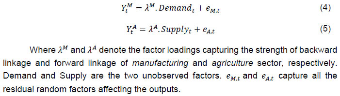 Now suppose in any period, manufacturing output increases by one unit due to some shock. Irrespective of whether this initial shock is demand or supply, the resultant increase in manufacturing output will lead to an increase in the demand factor (through equation 1). Additionally, the increased production in the manufacturing sector will increase demand for inputs from the agriculture sector. If the agriculture output increases in response, the supply factor will also increase (through equation 2), and demand-supply gap will be lower. In contrast, if the agricultural output does not rise in tandem, the supply factor will not increase and the demand-supply gap would widen, thereby fuelling inflation. Hence, by observing the output mix in the economy in any period and the sectoral inter-linkages, we can draw some information about the demand and supply, as defined in the paper. IV. Data We use quarterly national accounts data on sectoral GVAs (Agriculture, forestry & fishing; mining & quarrying; manufacturing; electricity, gas, water supply & other utility services; Construction; Trade, hotels, transport, communication and services related to broadcasting; financial, real estate & professional services; public administration, defence and other Services) and aggregate GVA at constant prices for the period: 2006:Q3 to 2020:Q113. The data transformation involves taking log and deseasonalising using X-13 ARIMA. Further, Hodrick-Prescott filter is applied to the data to extract sectoral cycles and aggregate (business) cycle. The Asian Development Bank data on the latest input-output table for the period 2017 are used in our analysis. This consists of 35 sectors, which we aggregate suitably14 to provide insights about the inter-relationships among the 8 GVA sectors (Appendix tables A1 and A2). V. Estimation and Results The complete set of equations used for estimation is given as follows: Since the purpose of the entire empirical exercise is to estimate demand and supply dynamics separately at business cycle frequency, HP-filtered (λ=1600) sectoral cycles are used to capture the sectoral dynamics. A Bayesian dynamic factor model is used to estimate this set of equations. We choose loose priors (Table 1) for the parameters, so that the estimated parameters are determined more by the data, rather than the choice of the priors. Further, we use the same priors for parameters pertaining to both demand and supply factors, in order to avoid any apriori statistical distinction between the two. The decomposition of the business cycle into demand and supply is depicted in Chart 4. 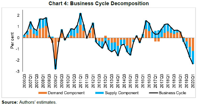 We now offer further evidence that the estimated indices are in fact representative of the demand-supply conditions in the economy. The first justification is based on the posterior estimates of the important parameters (Table 1). The estimates of AR1 and AR2 coefficients suggest that the estimated supply is more persistent than the estimated demand. This suggests that a supply shock will generate a more durable impact on output as compared to a demand shock. 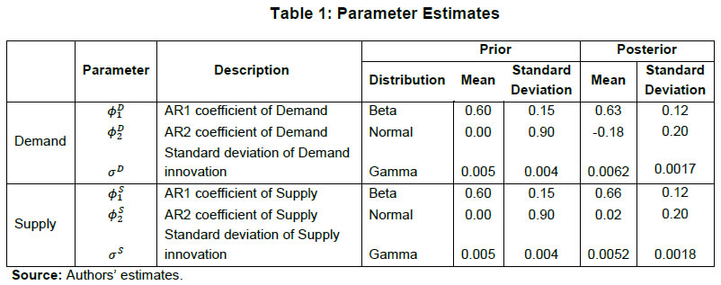 This is further corroborated by analysing the impulse response of output to average demand and supply shocks (chart 5), which suggests that most of the impact of demand shock fades away within 5 quarters while the impact of supply shock persists for more than 15 quarters. These findings are qualitatively similar to the seminal paper of Blanchard and Quah, 1988, which adopted the identification strategy that disturbances having temporary effect on output are deemed as demand while disturbances which have long-run impact on output are deemed to be of supply origin. 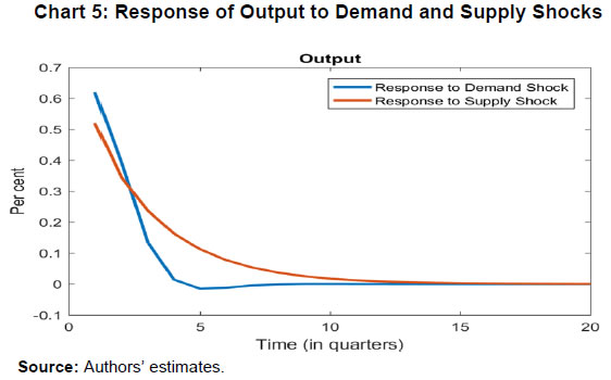 Second, a comparison of the standard deviation of innovations suggests that the estimated demand is more volatile than the estimated supply (Table 1). This property of the estimated demand-supply series is in line with the standard knowledge regarding demand and supply and generates confidence in our analysis. Third, the time-varying point estimates of demand-supply indices show that they track the actual major demand and supply events in the economy quite well (Chart 6). For example, the chart shows that the Global Financial Crisis of 2008-09 was marked by a sharper contraction in demand relative to supply. This is in line with the findings of Taylor and Benguria (2019) who concluded that financial crises “are very clearly a negative shock to demand”. During 2012-2014, the estimated indices showed a more pronounced drop in supply compared to demand. During this period, the economy was impacted by supply-side shocks like high oil prices and depreciation of the rupee on account of the taper tantrum. 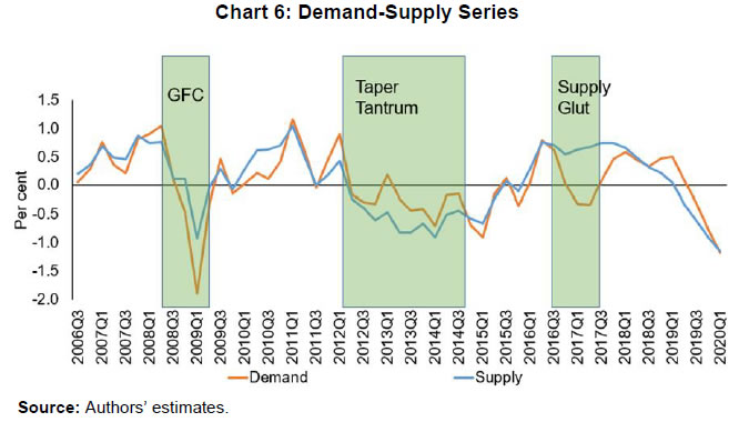 The final justification is based on the relationship of the estimated indices with inflation, which is explained in the next section. As we will see, the estimated indices are able to forecast inflation better than other measures of excess demand for the rolling sample considered in the study. VI. Relationship of estimated Demand-Supply Indices with Inflation CPI-Combined, which is the nominal anchor for monetary policy in India since the adoption of the flexible inflation targeting framework in 2016 is mainly composed of three subgroups: food (weight: 45.9 per cent), fuel (weight: 6.8 per cent), and excluding food and fuel (weight: 47.3 per cent). As a result of the substantial weight of food and fuel, headline inflation is highly susceptible to supply side shocks like erratic monsoons, transport disturbances, fuel prices, exchange rate changes, etc. (Chart 7). Apart from the direct effect through food and fuel, supply shocks also impact excluding food and fuel inflation via the cost-push channel (RBI, 2014). In order to assess if the estimated measure of macroeconomic demand-supply contains meaningful information about inflation, we construct a demand-supply mismatch (DSM) index by taking the difference of the demand and supply series. We see that the demand-supply mismatch index tracks headline inflation reasonably well (Chart 8). The contemporaneous correlation between the constructed measure and headline inflation is also higher compared to other popular measures of economic slack (Table 2). HP-output gap measures, which are frequently used as a measure of excess demand, show a negative (but insignificant) correlation with headline inflation. This is because headline, unlike core, is significantly affected by supply shocks. Without controlling for these supply-side effects, relation between HP-gap and headline inflation becomes weak. In contrast, the DSM index constructed by us contains information about both demand and supply, and hence proves to be a better measure. | Table 2: Correlation between Headline Inflation and Different Measures of Economic Slack | | | Demand-Supply Mismatch Index | GDP-gap (HP) | GVA-gap (HP) | OBICUS Capacity Utilization | Headline Inflation (CPI-C) | | Demand-supply mismatch Index | 1 | | | | | | GDP-gap (HP) | 0.094 | 1 | | | | | GVA-gap (HP) | (-) 0.01 | 0.91*** | 1 | | | | OBICUS Capacity Utilization | 0.28* | 0.61*** | 0.61*** | 1 | | | Headline Inflation (CPI-C) | 0.25* | (-) 0.12 | (-) 0.02 | 0.16 | 1 | Notes: * p < 0.10, ** p < 0.05, *** p < 0.01; Data for OBICUS capacity utilisation is taken from 2008:Q2 as per availability; HP-filtered OBICUS capacity utilisation cycle is used for correlation analysis.
Source: Authors’ estimates. | A more rigorous way of checking the association between DSM index and headline inflation would involve the regression framework. As a first step, we conduct the Granger-causality test to determine the direction of causality (Granger, 1969). Since Granger-causality analysis is based on VAR framework, it does not, apriori, require us to specify which variable is endogenous and which is exogenous. The results show that the DSM index Granger causes headline inflation while the headline inflation does not Granger cause DSM index (Table 3). The DSM index thus is an important explanatory variable for headline inflation. | Table 3: Granger-Causality Results | | Null Hypothesis: | (Obs:55) | F-Statistic | Prob. | | DSM does not Granger Cause Pi_headline | 2.34033 | 0.0851 | | Pi_headline does not Granger Cause DSM | 0.87186 | 0.4622 | | Source: Authors’ estimates. | Next, we regress headline inflation on the DSM index. We include alternative measures of slack in an ARIMA model for the regression15. We find that change in the DSM index by 1 percentage point causes a nearly equivalent change in headline inflation. We also run alternative specifications by replacing the DSM index with HP-output gap and capacity utilisation for comparison. In this case, the coefficients of these variables turn out to be insignificant (Table 4). | Table 4: Regression Results | Dependent
| (1) | (2) | (3) | | Independent | Pi_headline | Pi_headline | Pi_headline | | C | 1.754***
(0.373) | 1.729***
(0.352) | 0.433
(1.010) | | AR(1) | 0.853***
(0.121) | 0.811***
(0.138) | 0.964***
(0.027) | | MA(1) | -0.494**
(0.204) | -0.414*
(0.217) | -0.946***
(0.029) | | DSM | 1.018***
(0.378) | | | | HP-output gap | | 0.197
(0.136) | | | OBICUS Capacity Utilisation | | | 0.066
(0.047) | | Method | OLS | OLS | OLS | | Sample | 2006:Q3-2020:Q1 | 2006:Q3-2020:Q1 | 2008:Q3-2019:Q4 | | N | 55 | 55 | 47 | | Adj-R2 | 0.32 | 0.24 | 0.35 | Note: Standard errors in parentheses; * p < 0.10, ** p < 0.05, *** p < 0.01; ARMA specification is decided based on SIC criterion.
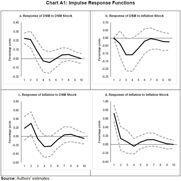
Source: Authors’ estimates. | In order to check if these results hold during periods of high inflation, the Granger-causality test was also carried out for the high inflation sub-sample (from 2006:Q3 to 2013:Q4). The results suggest that causality runs in both directions in this case (Table 5). As a result, a structural vector auto regression analysis of the two variables was conducted. A positive shock to DSM index fuels inflation with the impact being maximum at a quarter lag. On the other hand, an exogenous increase in inflation negatively affects the DSM index with the effect peaking at a lag of 3-4 quarters (Chart A1). | Table 5: Granger-Causality Results (for high inflation sub-sample) | | Null Hypothesis: | (Obs:30) | F-Statistic | Prob. | | DSM does not Granger Cause Pi_headline | 4.14734 | 0.0278 | | Pi_headline does not Granger Cause DSM | 2.72709 | 0.0849 | | Source: Authors’ estimates. | VI.1 Forecasting Exercise We would like to evaluate DSM index and other measures of excess demand in terms of their performance in forecasting headline inflation. As a first step, we determine the ARIMA specification that best describes the data generating process of headline inflation. We use this ARIMA specification for generating 1 to 4 quarters-ahead rolling forecasts. Subsequently, we nest this ARIMA specification with different measures of economic slack to form different bivariate models (of headline inflation and economic slack measures). The forecasting performance of these different bivariate models are then evaluated and compared to know whether the inclusion of economic slack helps predict headline inflation better or not. If it does, then which measure of economic slack does it the best? The general specification of the bivariate model is as follows: Total number of rolling samples are 10 while total length of our data is 28 quarters (2011Q1-2017Q4). This means we practically use 35 per cent of our data in conducting and evaluating out-of-sample forecasts. Moreover, the period 2015:Q4 to 2018:Q4 includes both upturns and downturns in economic slack (Chart 9). This ensures that forecasting evaluation/performance is independent of whether last period of the rolling sample is followed by an upturn or downturn in economic slack, and lends robustness and credibility to our forecasting results. A comparison of the RMSEs establishes the superior forecasting performance of the estimated DSM index vis-a-vis ARIMA and other measures of excess demand (Table 6). | Table 6: RMSE of Forecasts | | | Q1 | Q2 | Q3 | Q4 | | ARIMA/AR | 0.758 | 0.896 | 0.977 | 1.082 | | GDP-gap (HP) | 0.871 | 1.051 | 1.145 | 1.25 | | GVA-gap (HP) | 0.854 | 1.052 | 1.154 | 1.259 | | OBICUS Capacity Utilisation | 0.688 | 0.892 | 0.109 | 1.331 | | Demand-Supply Mismatch Index | 0.643 | 0.711 | 0.79 | 0.906 | | Source: Authors’ estimates. | VII. Conclusion From the perspective of inflation assessment, constructing a reliable measure of a demand-supply mismatch as an alternative to statistical measures of output gap and survey based measures of slack/capacity utilisation, and examining its usefulness in forecasting inflation is the key aim of this paper. To this end, this paper develops a framework to disentangle the role of demand-supply using a Bayesian DFM and the input-output tables. The demand-supply mismatch index is found to be positively correlated with headline inflation. Regression and Granger-causality results suggest that the estimated index exhibits a causal relationship with the headline inflation, and has superior inflation predictive power compared to other conventionally used measures of excess demand. Finally, we would like to mention that the fundamental idea underlying this paper like any other research effort, is likely to evolve over time. We have shown how linkages of a sector with other sectors determines to an extent its macroeconomic role in the economy. There can be many ways to improve the present analysis. For example, performing the same analysis with more granular data can allow better capturing of the inter-linkages present in the economy. We leave this and many other areas of further development to future research efforts in this domain.
References Benguria, F., & Taylor, A. M. (2019). After the panic: Are financial crises demand or supply shocks? Evidence from international trade (No. w25790). National Bureau of Economic Research. Berument, H., & Taşçı, H. (2002). Inflationary effect of crude oil prices in Turkey. Physica A: Statistical Mechanics and its Applications, 316(1-4), 568-580. Blanchard, O. J., & Quah, D. (1988). The dynamic effects of aggregate demand and supply disturbances (No. w2737). National Bureau of Economic Research. Chenery, H. B. & Watanabe, T. (1958). International Comparisons of the Structure of Production. Econometrica. Cover, J. P., Enders, W., & Hueng, C. J. (2006). Using the aggregate demand-aggregate supply model to identify structural demand-side and supply-side shocks: Results using a bivariate VAR. Journal of Money, Credit, and Banking, 38(3), 777-790. Enders, W., & Hurn, S. (2007). Identifying aggregate demand and supply shocks in a small open economy. Oxford Economic Papers, 59(3), 411-429. Granger, C. W. (1969). Investigating causal relations by econometric models and cross-spectral methods. Econometrica: Journal of the Econometric Society, 424-438. Guo, J., & Planting, M. A. (2000). Using input-output analysis to measure US economic structural change over a 24 year period. BEA. Hoffmaister, A. W., & Roldos, J. E. (1997). Are Business Cycles different in Asia and Latin America?. Jarocinski, M., & Lenza, M. (2015). Output gap and inflation forecasts in a Bayesian dynamic factor model of the euro area. Manuscript, European Central Bank. Kydland, F. E., & Prescott, E. C. (1982). Time to build and aggregate fluctuations. Econometrica: Journal of the Econometric Society, 1345-1370. Long Jr, J. B., & Plosser, C. I. (1983). Real business cycles. Journal of Political Economy, 91(1), 39-69. Miller, R. E., & Blair, P. D. (1985). Input-Output Analysis: Foundations and extensions Prentice-Hall. Englewood Cliffs, New Jersey. Miller, R. E., & Blair, P. D. (2009). Input-output analysis: foundations and extensions. Cambridge university press. Prescott, E. C. (1986, September). Theory ahead of business cycle measurement. In Carnegie-Rochester conference series on public policy (Vol. 25, pp. 11-44). North-Holland. Rand, J., & Tarp, F. (2002). Business cycles in developing countries: are they different?. World Development, 30(12), 2071-2088. RBI. (2014). Report of the Expert Committee to Revise and Strengthen the Monetary Policy Framework (Chairman: Urjit R. Patel), Reserve Bank of India. RBI (2020). Monetary Policy Report, October 2020, Reserve Bank of India, Mumbai. Reis, H., & Rua, A. (2009). An input–output analysis: Linkages versus leakages. International Economic Journal, 23(4), 527-544. Shapiro, M. D., & Watson, M. W. (1988). Sources of business cycle fluctuations. NBER Macroeconomics Annual, 3, 111-148. Spencer, D. E. (1996). Interpreting the Cyclical Behavior of the Price Level in the US. Southern Economic Journal, 95-105. Stock, J. H., & Watson, M. W. (2010). Modelling inflation after the crisis. National Bureau of Economic Research, No. w16488. Stock, J. H., & Watson, M. W. (2016). Core inflation and trend inflation. Review of Economics and Statistics, 98(4), 770-784. Wu, L., Li, J., & Zhang, Z. (2013). Inflationary effect of oil-price shocks in an imperfect market: A partial transmission input–output analysis. Journal of Policy Modeling, 35(2), 354-369.
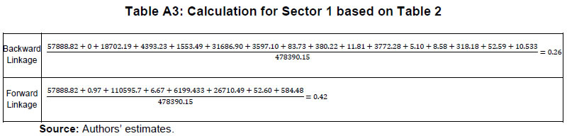
Appendix | Table A1: Categorization of the 35 Sectors of ADB Input-Output Table into the 8 GVA Sectors | | GVA Sector | Included Industries | | 1. Agriculture, forestry & fishing | Agriculture, Hunting, Forestry and Fishing | | 2. Mining & quarrying | Mining and Quarrying | | 3. Manufacturing | Food, beverages, and tobacco | | Textiles and textile products | | Leather, leather products, and footwear | | Wood and products of wood and cork | | Pulp, paper, paper products, printing, and publishing | | Coke, refined petroleum, and nuclear fuel | | Chemicals and chemical products | | Rubber and plastics | | Other non-metallic minerals | | Basic metals and fabricated metal | | Machinery, nec | | Electrical and optical equipment | | Transport equipment | | Manufacturing, nec; recycling | | 4. Electricity, gas, water supply & other utility services | Electricity, Gas and Water Supply | | 5. Construction | Construction | | 6. Trade, hotels, transport, communication and services related to broadcasting | Sale, maintenance, and repair of motor vehicles and motorcycles; retail sale of fuel | | Wholesale trade and commission trade, except of motor vehicles and motorcycles | | Retail trade, except of motor vehicles and motorcycles; repair of household goods | | Hotels and restaurants | | Inland transport | | Water transport | | Air transport | | Other supporting and auxiliary transport activities; activities of travel agencies | | Post and telecommunications | | 7. Financial, real estate & professional services | Financial intermediation | | Real estate activities | | Renting of M&Eq and other business activities | | 8. Public administration, defence and Other Services | Public administration and defense; compulsory social security | | Education | | Health and social work | | Other community, social, and personal services | | Private households with employed persons | | Source: MOSPI |
| Table A2: Constructed Input-Output Table with 8 GVA Sectors | | (current prices, $ million) | | | | | | | | | | | | | | Sectors | 1 | 2 | 3 | 4 | 5 | 6 | 7 | 8 | C | G | I | X | Total Output | | 1 | 57888.82 | 0.969894 | 110595.7 | 6.670567 | 6199.433 | 26710.49 | 52.60278 | 584.4812 | 259479.6 | 2544.165 | 931.736 | 13566.85 | 478390.2 | | 2 | 0 | 265.9236 | 60188.23 | 2928.697 | 1705.272 | 18.37793 | 0.867381 | 0.656283 | 83.6931 | 58.68155 | 0 | 9804.186 | 74433.94 | | 3 | 18702.19 | 9688.766 | 525432.3 | 10638.32 | 96903.9 | 113085.3 | 7989.149 | 16441.33 | 375689.3 | 21961.97 | 268338.5 | 240558.8 | 1809349 | | 4 | 4393.229 | 2872.926 | 38063.26 | 17397.87 | 4943.99 | 10853.88 | 4924.212 | 608.6612 | 11584.5 | 6120.444 | 0 | 129.6031 | 101892.6 | | 5 | 1553.491 | 1453.265 | 8958.581 | 1282.222 | 27419.99 | 5094.196 | 9235.088 | 1435.009 | 1031.928 | 2290.117 | 331796.9 | 570.0064 | 392120.8 | | 6 | 31686.9 | 6215.084 | 276034.4 | 11063.62 | 55911.21 | 116381.3 | 17380.44 | 15363.36 | 407579.4 | 15438.73 | 54046.06 | 35367.23 | 1042468 | | 7 | 3597.099 | 2933.225 | 83676.46 | 4739.988 | 13498.24 | 37690.87 | 32094.3 | 7048.443 | 242712.7 | 10409.93 | 15979.92 | 72299.45 | 526680.7 | | 8 | 83.73331 | 2260.082 | 20592.62 | 284.7844 | 205.2994 | 2266.626 | 5237.724 | 4940.945 | 199699.9 | 229310.7 | 0 | 11295.39 | 476177.8 | | | | | | | | | | | | | | | | | IMPORTS | | | | | | | | | | | | | | | 1 | 380.2256 | 4.578631 | 1975.734 | 1.121548 | 336.0716 | 193.037 | 61.60336 | 4.854429 | 2825.622 | 41.68576 | 12.75222 | | 5854.205 | | 2 | 11.81766 | 995.3504 | 122501.9 | 8026.296 | 3055.974 | 120.8285 | 7.008911 | 13.56148 | 283.5498 | 202.9182 | 52.35158 | | 135300.7 | | 3 | 3772.281 | 1622.799 | 106792.3 | 1551.678 | 11067.72 | 15767.54 | 2225.769 | 4068.952 | 14932.75 | 2062.945 | 40070.84 | | 211059.4 | | 4 | 5.098364 | 5.541876 | 574.3282 | 34.05879 | 26.15411 | 19.19122 | 11.14002 | 3.45597 | 15.78755 | 2.250892 | 23.77051 | | 725.2213 | | 5 | 8.585114 | 16.43968 | 859.3789 | 57.51373 | 131.7262 | 45.37106 | 33.77259 | 11.47511 | 7.502987 | 2.191013 | 50.80602 | | 1230.297 | | 6 | 318.1836 | 132.1571 | 11545.4 | 529.41 | 908.6133 | 1136.363 | 455.5195 | 202.3124 | 3105.785 | 341.889 | 1573.655 | | 21187.36 | | 7 | 52.59118 | 123.3478 | 4749.719 | 192.9509 | 1169.053 | 2543.471 | 2259.017 | 371.6621 | 681.8265 | 122.6581 | 355.8523 | | 12717.04 | | 8 | 10.53306 | 259.0747 | 1005.374 | 49.62719 | 161.6325 | 461.1047 | 849.2141 | 356.8234 | 2526.16 | 848.7023 | 49.72225 | | 6593.255 | | | | | | | | | | | | | | | | | Value added at basic prices | 371178.3 | 43899.39 | 351525.4 | 41059.97 | 143313.5 | 670217.3 | 439366.9 | 421029.6 | | | | | 2481590 | | Output at basic prices | 478390.2 | 74433.94 | 1809349 | 101892.6 | 392120.8 | 1042468 | 526680.7 | 476177.8 | 1564777 | 302472.2 | 757499.8 | 383591.5 | 8021209 | | Source: Authors’ estimates. |
 |