Press Release

RBI Working Paper Series No. 15

Measuring Trend Inflation in India

Harendra Kumar Behera and Michael Debabrata Patra^@

Abstract

^*Central to monetary policy is the concept of trend inflation to which actual inflation outcomes are expected to converge after short run fluctuations die out. Accordingly, the inflation target needs to be fixed in alignment with trend inflation to avoid unhinging inflation expectations and flattening the aggregate supply curve or imparting a deflationary bias to the economy. Results from a regime switching model applied to a hybrid New Keynesian Philips curve suggest a steady decline in trend inflation since 2014 to 4.1-4.3 per cent just before COVID-19 struck. This points to maintaining the inflation target at 4 per cent for India.

JEL Classification: C22, E31, E42, E52, E58.

Keywords: Trend inflation; Inflation target; Regime-switching model; Stochastic volatility

Introduction

Central to the design and conduct of monetary policy is the concept of trend or steady state inflation, the level to which actual inflation outcomes are expected to converge after short run fluctuations from a variety of sources, including shocks, die out¹. It provides key insights for monetary policy wielders in at least three important ways. First, the level and variability of trend inflation indicate how anchored inflation expectations are (Garnier, Mertens and Nelson, 2015). Second, it is a valuable gauge of the appropriateness of the monetary policy stance and the necessity or otherwise of additional monetary policy actions to achieve steady state inflation (Okimoto, 2018). The crucial question is: is the inflation target consistent with trend inflation which is, itself, time varying? Third, trend inflation provides a centering point for the evaluation of inflation forecasts over various time periods and, this in turn, can usefully inform the setting of monetary policy (Garnier et al., 2015).

Not surprisingly, trend inflation is regarded as a key building block of the new Keynesian model that is at the core of the monetary policy frameworks of modern central banks across the world. In particular, it is seen as influencing the shape and slope of the economy’s aggregate supply curve. The new Keynesian Phillips curve (NKPC), which has found intuitive appeal for its micro-foundations and its forward-lookingness² (Mavroeidis, Plagborg-Muller and Stock, 2014), is typically specified in a ‘gap’ formulation: the inflation gap i.e., deviations of actual inflation from a time varying trend rather than from a constant mean. This is equivalent to writing the NKPC as raw inflation with a drift term that depends on trend inflation (Yun, 1996).

Understanding persistence or the tendency of inflation to converge slowly to its trend is also critical to fashioning appropriate monetary policy responses in terms of the size and timing of policy actions. Early efforts to model persistence through univariate autoregressive models (Fuhrer and Moore, 1995; Nelson and Plosser, 1982) were found to yield biased estimates, since they only measured ‘intrinsic’ persistence or backward-lookingness in price formation. More recent research identifies four sources of inflation persistence: intrinsic; extrinsic i.e., inherited from the mark-up over costs imparted by the state of the economy; expectations-based; and, policy induced or resulting from monetary policy itself (Angeloni et al., 2006)³. Judging the time taken by inflation to approach its trend after a shock requires knowledge of how short-run fluctuations decay as well as how longer-lived fundamentals associated with monetary policy affect expectations and drive inflation. In fact, considerable evidence has been accumulated on a substantial portion of inflation persistence being accounted for by variations in trend inflation which could emanate from monetary policy regime shifts (Stock and Watson, 2007; 2010; Morley, Piger and Rasche, 2015).

In the context of this paper, trend inflation serves the crucial purpose of a consistency check on the setting of inflation targets. Illustratively, if the inflation target is fixed too much higher than trend inflation, observed inflation would run higher and become more volatile. This could unhinge inflation expectations and risk premia in financial markets would rise (Bernanke, 2010). It could also increase price dispersion, flatten the aggregate supply curve and amplify the impact of monetary policy shocks, squandering hard-won inflation credibility. Should trend inflation itself rise because of the central bank persisting in setting a target higher than trend, monetary policy can become less effective in stabilising the economy (Ascari and Ropele, 2007). These costs have to be weighed against the advantages of avoiding the zero lower bound on interest rates that higher targets seek to address⁴. Per contra, setting inflation target too much below trend imparts a deflation bias to the economy, inflation expectations and financial markets, blunting the efficacy of monetary policy in its symmetrical stabilising role. The optimal approach is to set the inflation target in broad alignment with or slightly below trend inflation.

Measuring trend inflation is essentially an empirical issue (Garnier et al, 2015; Ascari and Sbordone, 2014; Beveridge and Nelson, 1981). Attention is being increasingly given to precision in modelling the time-varying dynamics of trend inflation including structural shifts therein. Ab initio, the effort needs to be recognised as difficult because it deals with an ‘unobservable’. As presciently pointed out, it involves filtering out the noise in inflation data, but there are multiple sources of noise that can change over time. Thus, it embodies a signal extraction problem, which becomes complicated when trend inflation itself is time varying (Stock and Watson, 2016).

Nonetheless, estimating trend inflation with regular updates is important for the formulation of monetary policy, irrespective of the country setting. In India, this exercise acquires priority in the context of the flexible inflation targeting formally instituted in June 2016, which commits the central bank – the Reserve Bank of India (RBI) – to a consumer price inflation target of 4 per cent with a symmetrical tolerance band of +/- 2 per cent around it. Moreover, section 45ZA of the Reserve Bank of India Act, 1934 mandates that the Central Government shall, in consultation with the Bank, determine the inflation target once in every five years. Accordingly, the inflation target has to be reviewed by end-March 2021. In this context, trend inflation provides the metric to gauge the appropriate level of the target going forward.

Against this backdrop, this paper reviews the behaviour of trend inflation in India. Given the specific features of the Indian experience, Section II of the paper undertakes an exploration of the rich empirical literature to draw the rationale for our choice of methodology of a regime-switching model applied to a hybrid NKPC to capture trend inflation dynamics. Section III sets out the methodology, the data, variables and period of study. Section IV presents the empirical results, including the effects of the methodological innovations we bring in to overcome limitations of competing approaches. In brief, our results suggest a steady decline in trend inflation since 2014 to 4.1-4.3 per cent just before the outbreak of COVID-19. Section V summarises our efforts and offers some policy perspectives that we gleaned while developing this paper.

II. Choice of Methodology

In keeping with the main purpose of this paper, we investigate regime shifts in the dynamics of trend inflation in order to secure precision in estimates. The choice of the appropriate methodology for application in the Indian context needs to be informed by the historical evolution of the technology for estimating trend inflation, while incorporating underlying variations in time and space.

In the theoretical literature, the standard approach has been to assume zero trend inflation in the steady state. In the empirical literature, however, a non-zero trend inflation is preferred and a wide variety of models for estimating trend inflation from the data is available. Survey-based data on inflation expectations have been used (Clark, 2011; Kozicki and Tinsley, 2012; Faust and Wright, 2013), but estimates of trend inflation therefrom suffer from various biases in the survey responses (Clark and Doh, 2014; Kaihatsu and Nakajima, 2018). Survey-based approaches also lack several positive features of a model such as ascertaining the determinants of trend inflation and obtaining a forecast when needed. Elsewhere, trend inflation has been measured by the last period’s inflation rate (Brayton, Roberts and Williams, 1999); as a random walk (Cogley, Primericeri and Sargent, 2010; Stock and Watson, 2010; Mertens, 2011); a random walk subject to bounds (Chan, Koop and Potter, 2013); and as an exponentially smoothed trend.

The workhorse model for estimating trend inflation, and arguably the most popular, has been the unobserved components with stochastic volatility (UCSV) model (Stock and Watson, 2002; 2007; 2010). Confining itself to studying the dynamics driving a single measure of inflation, it adopts the elegant decomposition of a non-stationary time series into permanent and transitory components, with the former identified as the trend and the latter as the cycle (Beveridge and Nelson, 1981). The trend is defined as a random walk⁵ process, while the inflation gap is governed by a separate process of stochastic volatility. Variations in the inflation gap – the difference between trend and observed inflation – are assumed to be serially uncorrelated, i.e., it has no persistence. In essence, therefore, in univariate time-varying trend-cycle models with stochastic volatility, the dynamics of inflation are largely dominated by the trend component. It is equivalent to a time-varying first order integrated moving average [IMA (1,1)] inflation model (Stock and Watson, 2007). The IMA (1,1) adapts less quickly, however, to changing parameters than the UCSV model.

Extension of the UCSV model has involved a so-called ‘multivariate’ approach in which different series of inflation-measuring metrics – CPI; GDP deflator – are pooled and a common trend is identified and extracted, but with trend levels differing in recognition of discrepancies across inflation metrics due to a variety of factors, including construction, coverage and the like, though only by a constant. Designated as the multivariate stochastic volatility (MVSV) model, it nests the UCSV model, but unlike the latter, it allows the inflation gap to exhibit persistence albeit with convergent dynamics. Shocks to individual gap volatilities are allowed to be correlated with each other while allowing for idiosyncratic changes in the behaviour of individual inflation measures. Work in this strain may allow inflation gap persistence to vary with time (a la Cogley, Primiceri and Sargent, 2010) or may adopt a more parsimonious approach in which the coefficient on inflation gap persistence is held constant or time-invariant in the parametric sense. The measurement equation of the MVSV model has also been augmented with inflation targets, the latter being interpreted as a direct reading of a deterministic trend.

The MVSV model itself has been extended to the application of time series smoothing methods to cross-sectional inflation data to derive estimates of trend inflation that correspond to the standard measure of core inflation (Kiley, 2008; Stock and Watson, 2016). These models improve upon the standard UCSV prototype by including explicit model-based treatment of outliers. They also allow for a common latent factor in both the trend and transitory components in the underlying cross-sectional series (e.g., constituents of the personal consumption expenditure deflator of the US) as well as time varying factor loadings that allow for changes in correlations across constituent series. The aggregate trend inflation is the sum of sectoral trends weighted by shares in total inflation. These models have been estimated by using Bayesian methods. Multivariate trend estimates turn out to be more precise that univariate estimates, but the latter can match up in accuracy when applied directly to core measures of inflation. Moreover, out-of-sample improvements in forecasting of the multivariate models are modest relative to those that use headline inflation alone. Other work in this tradition has sought to extract a common trend in inflation rates, surveys and nominal yields (Mertens, 2011).

The UCSV and MVSV models exhibit broad similarities in capturing similar low-frequency movements and in producing similar estimates of the inflation trend and its stochastic volatility. In the face of large shocks such as the global financial crisis (GFC), however, UCSV estimates are observed to be affected by transitory fluctuations in inflation from which the MVSV model insulates its trend estimates and instead, lets them be captured in the inflation gap. This is important from the point of view of separating sustained overshoots/undershoots of the inflation target from the phenomenon of shifts in the trend. Thus, MVSV trend estimates tend to be smoother and less variable than their UCSV counterparts and are also associated with lower average forecast errors.

The UCSV/MVSV models are observed to be too flexible, undermining the plausibility of the estimate of trend inflation that is obtained; they are also heavily dependent on the prior distribution of stochastic volatility (Kaihatsu and Nakajima, op cit). Moreover, while these models essentially draw out trend inflation from the series of a single inflation measure or from a set of inflation measures, they do not attempt to draw information that may be contained in other economic variables. This may be redundant from the point of view of the forecasting properties of these models; in fact, it is documented in the literature that the contribution of real variables to the forecasting of inflation is rather modest (Stock and Watson, 2009; Faust and Wright, 2013). In the context of monetary policy analysis, however, this feature emerges as a shortcoming. In the real world, inflation persistence could be correlated with persistence in other macroeconomic variables, especially the output gap. In fact, such interactions are crucial for the setting of monetary policy. Accordingly, it is to this class of trend inflation models that we now turn.

A recent strand in the empirical literature on the subject has sought to estimate trend inflation by modeling it as an unobserved state variable that is influenced/ determined by extrinsic macroeconomic conditions embodied in the Phillips curve. In seminal work in this vein, Bayesian VARs with drifting coefficients have been employed to estimate trend inflation from the joint interactions of inflation, unemployment rate and the short-term nominal interest rate, while accounting for stochastic volatility (Cogley and Sargent, 2001; 2005). Consistent with univariate models, this work found that most of the volatility in inflation is in the trend component, with innovations accounting for only a small fraction of the unconditional variance of inflation. Two main approaches are discernible in this strand. One is the time varying parameter VAR model, but the main criticism is that flexible assumptions regarding parameter evolution can lead to over-parameterisation (Koop, Leon-Gonzales and Strachan, 2009). This approach has also been found to be vulnerable to misspecification of the VAR restriction (Nason and Smith, 2008). In the other approach, regime shifts in monetary policy are introduced into the Phillips curve through a Markov Chain Monte Carlo (MCMC) process. A smooth transition model is generally preferred over the imposition of zero restrictions on transition probabilities in order to account for possible permanent regime changes such as the adoption of FIT as well as temporary shifts like quantitative easing after which trend inflation reverts to its stationary state (Okimoto, 2019). Alternatively, an equally spaced transition has been employed, consistent with the practice of expressing inflation targets and expectations as integers (Kaihatsu and Nakajima, 2018). Rather than a purely forward-looking NKPC advocated in the theoretical literature, a hybrid Phillips curve is preferred in which current inflation depends on trend inflation, the current output gap and past inflation to account for backward-looking price setting behaviour influenced by histories of high inflation. Trend inflation evolves as a drift-less random walk (Ascari and Sbordone, 2014). Again, Bayesian analysis and computation appears to be the preferred approach.

To sum up, drawing on influential categorization (Stock and Watson, 2009), models for estimating trend inflation can be grouped into three broad categories: (a) univariate models, including non-linear or time-varying specifications, and those that draw upon one or more inflation measures; (b) models based on expectations drawn from surveys and financial asset prices; and (c) models based on activity variables embedded in the Phillips curve. UCSV/MVSV models and their variants score in terms of forecasting performance or at least competing models have not been able to improve materially over univariate models. Where they fall short, however, is that they do not link time-series properties of inflation to more fundamental changes in the economy, especially those that stem from the changes in the conduct of monetary policy, in the structure of the real economy and the deepening of financial markets. All these factors can induce deep-seated changes in inflation dynamics. For instance, the progressive shift in the stance of monetary policy stance from a reactive to a forward-looking one has been widely credited with anchoring inflation expectations and downward shifts in the behavior of trend inflation.

III. The Model and Estimation Strategy

For the purpose of estimating trend inflation in India in the presence of shifts in inflation dynamics, a hybrid New Keynesian Phillips curve (NKPC)⁶ is employed in which current inflation depends on lagged inflation to capture the historical intrinsic behaviour of the inflation process, trend inflation to reflect persistence in inflation expectations and the contemporaneous output gap to represent the extrinsic macroeconomic conditions relevant for the setting of monetary policy (Gali and Gertler, 1999; Christiano, et al., 2005). The hybrid NKPC is specified as follows: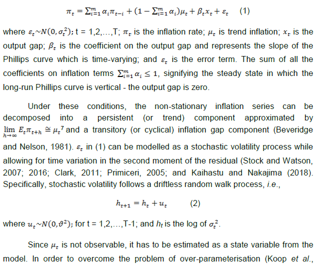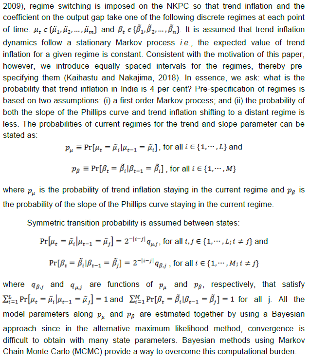

Trend inflation regimes are assumed to take the values of 2, 3, 4, …, 6, with a gap of 1 between two sequential regimes. The range of the pre-specified regimes for trend inflation is derived from a Hodrick-Prescott filter of realised inflation. Similarly, the slope of the Phillips curve is assumed to take a decimal number with the values being equally spaced, i.e. 0.05,…. 0.35 with a gap of 0.05 between two consecutive regimes⁸. The lag length of the inflation series eq. (1) is selected as 4, based on the

Filtered as well as smoothed posterior regime probability estimates are presented. While it is a common practice to present the results in terms of smoothed estimates only, filtered or real-time estimates are also useful as they reflect future information on state variables.

Using the posterior regime probabilities as weights, average trend inflation and average Phillips curve slope coefficients are computed as time-varying estimates.

IV. Data and Estimation Results

The use of quarterly data on various variables in the empirical analysis is mainly governed by the availability of GDP data. Accordingly, monthly data on the consumer price index (CPI) are averaged to produce quarterly data on inflation. Quarterly GDP data on the Indian economy are available from 1996. For data of older vintage so as to capture historical properties, annual data from 1980 are transformed into quarterly frequency using temporal disaggregation (Chow and Lin, 1976). Estimates of the output gap are obtained by first applying a battery of filters, i.e., the Hodrick-Prescott filter, the Band Pass (BP) filter (Baxter and King, 1999), the asymmetric BP filter (Christiano and Fitzgerald, 2003) and a multivariate Kalman filter (with Philips curve) on GDP data and then combining the estimates therefrom by principal components to produce a composite measure of the output gap. All data were sourced from the Handbook of Statistics on the Indian Economy (RBI at https://www.rbi.org.in).

The output gap and the inflation rate turned out to be visually volatile (Chart 1), although the amplitude of fluctuations in the inflation rate appears to have reduced over time, especially with the adoption of flexible inflation targeting. The output gap slipped into negative territory from January-March 2020, ahead of the onset of the pandemic in India, which reflects the weak state of the economy caught in the throes of an 8-quarter cyclical slowdown even before COVID-19 struck.

Before estimating the NKPC model with pre-specification of regimes, a Markov switching regression with unknown regimes is estimated to understand the current regime of inflation. The model is estimated by assuming the error variance to be different across regimes. The result indicates two regimes in India’s recent inflation history – a high inflation regime of 9.4 per cent during 2007-2014 and a low inflation regime of 4.0 per cent since 2015 (Chart 2). The probability of weighted estimate of trend inflation in the current regime is 4.2 per cent.

Bayesian estimation is conducted with priors for various parameters and the values of equally-spaced regimes for trend inflation and slope of the Philips curve (Table 1)⁹. The sum of the AR coefficients is 0.9, indicating that inflation is highly persistent in India. The stochastic volatility for the full sample period is quite large at 2.3, implying that the inflation process in India is vulnerable to repetitive supply shocks, some of which are large relative to the cross-country experience reported in the literature. The posterior regime probability of trend inflation indicates that the smoothed probability for the regime of 4 per cent increased after 2012 (Chart 3)¹⁰.

These results are intuitively appealing as the regime switch dates coincide with the de facto adoption of pre-conditions for inflation targeting in 2014, followed by the de jure institution of flexible inflation targeting (FIT) by legislative mandate in June 2016, with headline CPI inflation of 4 per cent as the primary objective of monetary policy in India.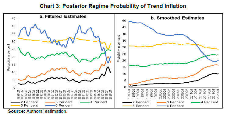

Chart 4 plots the filtered and smoothed posterior estimate-based weighted average trend inflation rates with their respective one standard deviation bands. The real time estimate of trend inflation declined steadily after 2013 after to 4.1 per cent in Q1 of 2019, before inching up thereafter during the COVID-19 pandemic (Chart 4). Smoothed probability estimates weighted average trend inflation – our preferred trend inflation estimates – eased steadily after 2009 and reached 4.3 per cent in Q1 of 2020. It is worthwhile to note that trend inflation still remains above the target under FIT, although it is on a declining trajectory. This indicates that inflation expectations are not yet fully anchored to the target but convergence is underway.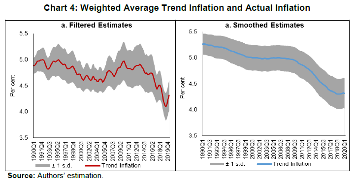

The steady decline in trend inflation is consistent with the flattening of the Philips curve that is reflected in the gradual fall in its slope parameter (Chart 5). The coefficient on the output gap works out to about 1, when error correction effects are taken into account, which indicates the exploitable trade-off for monetary policy in its standard stabilisation role.

Stochastic volatility shows a cyclical pattern, which has an important bearing on forecasting inflation (Chart 6). The steady decline in stochastic volatility from about 11 by end of 1990s to 4.4 in 2008-09:Q3 and further to around 2 in 2016-17:Q1 and remaining flat thereafter suggests a decline in the influence of supply shocks on inflation. This also suggests a growing credibility associated with the conduct of monetary policy.

The historical decomposition of observed inflation suggests a dominant share of trend inflation in overall variations (Chart 7), with occasional spikes on account of stochastic shocks. These findings underscore the role of trend inflation and stochastic volatility in understanding overall inflation dynamics.

V. Conclusion

This paper began with a question that goes to the root of FIT in India – is the choice of the target for inflation consistent with its trend? A target set below the trend imparts a deflationary bias to monetary policy because it will go into overkill relative what the economy can intrinsically bear in order to achieve the target. Analogously, a target that is fixed above trend renders monetary policy too expansionary and prone to inflationary shocks and unanchored expectations.

Trend inflation is an empirical question and choice of methodology is crucial if the estimate of trend inflation has to be precise. Within the proliferation of work on the subject, there is a loose consensus that none of them can outperform the random walk model for forecasting purposes. For the setting of monetary policy, however, it is necessary to consider significant changes in the overall macroeconomic ecosystem in which monetary policy is conducted. In this regard, Markov switching offers a computationally lighter alternative without sacrificing precision.

Trend inflation was falling even ahead of the institution of FIT and the latter entrenched this tendency, as reflected in the rising probability of trend inflation at 4 per cent in both filtered and smoothed posterior estimates. The probability-weighted average of trend inflation has come down after 2014 – when the pre-conditions of FIT were beginning to be put in place – to 4.1-4.3 per cent in Q1 of 2020, just before COVID-19 struck.

The decline in trend inflation since 2014 is, however, coincident with a flattening of the Philips curve. Underlying this is (a) a decline in the inflation persistence, indicating that households and businesses in India are becoming more forward-looking than before as credibility associated with monetary policy increases; and (b) an increase in sacrifice ratio – further disinflations will become costlier in terms of the output foregone. At the same time, the credibility bonus accruing to monetary policy warrants smaller policy actions to achieve the target. This points to maintaining the inflation target at 4 per cent into the medium-term. If it ain’t broke, don’t fix it.

^@ The authors are from Reserve Bank of India and the views expressed in this paper are those of the authors and not necessarily those of the institution to which they belong.

^* Comments and suggestions received from Shesadri Banerjee, Binod Bhoi, Joice John, Mridul Saggar, Sanjay Hansda, Jai Chander and Jugnu Ansari are gratefully acknowledged. The authors would like to express their gratitude to Jouchi Nakajima, Bank of Japan for sharing his Ox code.

¹ The terms ‘trend’, ‘steady state’ and ‘expected’ inflation will be used interchangeably through the rest of the paper.

² Current inflation is determined by expected future inflation and marginal cost. Difficulties in fitting the purely forward-looking NKPC led to specifications with lagged inflation terms to capture intrinsic persistence in the inflation formation process (Gali and Gertler, 1999; Christiano et al., 2005; Sbordone, 2005; 2007) – the so-called hybrid NKPC.

³ Empirical analysis of the sources of inflation persistence in India found that the role of inflation expectations has increased in driving inflation persistence during the post-GFC period (Patra et al., 2014).

⁴ In this context, the recent debate on the appositeness of the level of the inflation target – 4 per cent, as against the current 2 per cent in the US - has stirred considerable excitement and impassioned viewpoints (Blanchard, et al., 2010; Bernanke, 2010; Ball, 2013).

⁵ A random walk refers to any process in which there is no observable pattern or trend, i.e., where the movements of an object, or the values taken by a certain variable, are completely random. The best example of a random walk is that of a drunk person walking home from a bar on a Saturday night.

⁶ The literature also provides empirical validation of NKPC in the Indian context (Patra and Ray, 2010; Patra and Kapur, 2012; Sahu, 2013; Patra et al. 2014; Salunkhe and Patnaik, 2019; Pattanaik et al., 2020) wherein inflation is largely determined by intrinsic persistence, with the role of inflation expectations and monetary policy having increased in post-GFC period (Patra et al. 2014).

⁷ Over an infinite horizon, inflation is expected to converge to its trend value.

⁸ The regime values for the slope of the Phillips curve is assumed on the basis of the slope coefficients of a rolling regression of actual inflation on an intercept, lagged inflation and output gap. The estimates are broadly in line with the values found in the empirical literature in the Indian context.

⁹ Various diagnostic tests confirm the convergence of the parameters with autocorrelation decaying faster to zero and the trace plot for each parameter is converging to the mean value.

¹⁰ Using data for 1996:Q2 to 2019:Q4 (i.e. excluding the period of unavailability of official quarterly GDP estimates and 2020:Q1 when COVID-19 started in India) and inflation regime values of 1 to 9 per cent, the results show the highest probability for 4 per cent regime. The probability has increased sharply since Q1 of 2014. The results based on core inflation even show a much clearer picture. The results are provided in Annex I.

Reference

Angeloni, I., Aucremanne, L., Ehrmann, M., Galí, J., Levin, A., & Smets, F. (2006). New Evidence on Inflation Persistence and Price Stickiness in the Euro Area: Implications for Macro Modeling. Journal of the European Economic Association, 4(2-3), 562-574.

Ascari, G., & Ropele, T. (2007). Optimal Monetary Policy under Low Trend Inflation. Journal of monetary Economics, 54(8), 2568-2583.

Ascari, G., & Sbordone, A. M. (2014). The Macroeconomics of Trend Inflation. Journal of Economic Literature, 52(3), 679-739.

Baxter, M., & King, R. G. (1999). Measuring Business Cycles: Approximate Band-Pass Filters for Economic Time Series. Review of Economics and Statistics, 81(4), 575-593.

Bernanke, B. S. (2010). Opening Remarks: The Economic Outlook and Monetary Policy. In Proceedings-Economic Policy Symposium-Jackson Hole (pp. 1-16). Federal Reserve Bank of Kansas City.

Beveridge, S., & Nelson, C. R. (1981). A New Approach to Decomposition of Economic Time Series into Permanent and Transitory Components with Particular Attention to Measurement of the ‘Business Cycle’. Journal of Monetary Economics, 7(2), 151-174.

Brayton, F., Roberts, J. M., & Williams, J. C. (1999). What's happened to the Phillips curve?. Federal Reserve Board FEDS Working Paper, No. 1999-49, url: https://www.federalreserve.gov/Pubs/feds/1999/199949/199949pap.pdf

Chan, J. C., Koop, G., & Potter, S. M. (2013). A New Model of Trend Inflation. Journal of Business & Economic Statistics, 31(1), 94-106.

Chow, G. C., & Lin, A. L. (1976). Best Linear Unbiased Estimation of Missing Observations in an Economic Time Series. Journal of the American Statistical Association, 71(355), 719-721.

Christiano, L. J., & Fitzgerald, T. J. (2003). The Band Pass Filter. International Economic Review, 44(2), 435-465.

Christiano, L. J., Eichenbaum, M., & Evans, C. L. (2005). Nominal Rigidities and the Dynamic Effects of a Shock to Monetary Policy. Journal of political Economy, 113(1), 1-45.

Clark, T. E. (2011). Real-time Density Forecasts from BVARs with Stochastic Volatility. Journal of Business and Economic Statistics, 29, 327-341.

Clark, T. E., & Doh, T. (2014). Evaluating Alternative Models of Trend Inflation. International Journal of Forecasting, 30(3), 426-448.

Cogley, T., & Sargent, T. J. (2001). Evolving Post-World War II US Inflation Dynamics. NBER Macroeconomics Annual, 16, 331-373.

Cogley, T., & Sargent, T. J. (2005). Drifts and Volatilities: Monetary Policies and Outcomes in the Post WWII US. Review of Economic Dynamics, 8(2), 262-302.

Cogley, T., Primiceri, G. E., & Sargent, T. J. (2010). Inflation-gap Persistence in the US. American Economic Journal: Macroeconomics, 2(1), 43-69.

Faust, J., & Wright, J. H. (2013). Forecasting Inflation. In Handbook of Economic Forecasting (Vol. 2, pp. 2-56). Elsevier.

Fuhrer, J., & Moore, G. (1995). Inflation Persistence. The Quarterly Journal of Economics, 110(1), 127-159.

Gali, J., & Gertler, M. (1999). Inflation Dynamics: A Structural Econometric Analysis. Journal of monetary Economics, 44(2), 195-222.

Garnier, C., Mertens, E., & Nelson, E. (2015). Trend Inflation in Advanced Economies. International Journal of Central Banking, 11, 66-136.

Kaihatsu, S., & Nakajima, J. (2018). Has trend inflation shifted?: An Empirical Analysis with an Equally-spaced Regime-switching Model. Economic Analysis and Policy, 59, 69-83.

Kiley, M. T. (2008). Estimating the Common Trend Rate of Inflation for Consumer Prices and Consumer Prices excluding Food and Energy Prices. Finance and Economics Discussion Series 2008-38. Board of Governors of the Federal Reserve System (U.S.).

Koop, G., Leon-Gonzalez, R., & Strachan, R. W. (2009). On the Evolution of the Monetary Policy Transmission Mechanism. Journal of Economic Dynamics and Control, 33(4), 997-1017.

Kozicki, S., & Tinsley, P. A. (2012). Effective use of Survey Information in Estimating the Evolution of Expected Inflation. Journal of Money, Credit and Banking, 44(1), 145-169.

Mavroeidis, S., Plagborg-Muller, M., & Stock, J. H. (2014), Empirical Evidence on Inflation Expectations in the New Keynesian Phillips Curve. Journal of Economic Perspectives, 52(1), 124-188.

Mertens, E. (2011). Measuring the Level and Uncertainty of Trend Inflation. Federal Reserve Board FEDS Working Paper, No. 2011-42.

Morley, J., Piger, J., & Rasche, R. (2015). Inflation in the G7: Mind the Gap (s)?. Macroeconomic Dynamics, 19(4), 883.

Nelson, C. R., & Plosser, C. R. (1982). Trends and Random Walks in Macroeconomic Time series: some evidence and implications. Journal of Monetary Economics, 10(2), 139-162.

Okimoto, T. (2019). Trend Inflation and Monetary Policy Regimes in Japan. Journal of International Money and Finance, 92, 137-152.

Patra, M.D., & Ray, P. (2010). Inflation Expectations and Monetary Policy in India: An Empirical Exploration. IMF Working Papers, No. 10/84, 1-26.

Patra, M.D., Khundrakpam, J.K. & George, A.T. (2014). Post-Global Crisis Inflation Dynamics in India, What has Changed?. India Policy Forum, 2013–140 (10), 117-191.

Pattanaik, S., Muduli, S., & Ray, S. (2020). Inflation Expectations of Households: Do They Influence Wage-price Dynamics in India?. Macroeconomics and Finance in Emerging Market Economies, 1-20.

Sahu, J. P. (2013). Inflation Dynamics in India: A Hybrid New Keynesian Phillips curve Approach. Economics Bulletin, 33(4), 2634-2647.

Salunkhe, B., & Patnaik, A. (2019). Inflation Dynamics and Monetary Policy in India: A New Keynesian Phillips Curve Perspective. South Asian Journal of Macroeconomics and Public Finance, 8(2), 144-179.

Sbordone, A. M. (2005). Do Expected Future Marginal Costs drive Inflation Dynamics?. Journal of Monetary Economics, 52(6), 1183-1197.

Sbordone, A. M. (2007). Inflation Persistence: Alternative Interpretations and Policy Implications. Journal of Monetary Economics, 54(5), 1311-1339.

Stock, J. H., & Watson, M. W. (2002). Has the Business Cycle Changed and Why?. NBER Macroeconomics Annual, 17, 159-218.

Stock, J. H., & Watson, M. W. (2007). Why has US Inflation Become Harder to Forecast?. Journal of Money, Credit and banking, 39, 3-33.

Stock, J. H., & Watson, M. W. (2009). Phillips Curve Inflation Forecasts. In Understanding Inflation and the Implications for Monetary Policy: A Phillips Curve Retrospective, proceedings of FRB Boston's 2008 annual economic conference. Cambridge, MA: MIT Press.

Stock, J. H., & Watson, M. W. (2010). Modeling Inflation After the Crisis. NBER Working Paper Series, No. 16488, National Bureau of Economic Research.

Stock, J. H., & Watson, M. W. (2016). Core Inflation and Trend Inflation. Review of Economics and Statistics, 98(4), 770-784.

Yun, T. (1996). Nominal Price Rigidity, Money Supply Endogeneity, and Business Cycles. Journal of monetary Economics, 37(2), 345-370.

Annex I: Alternative Estimates of Trend Inflation

The estimates are based on data for 1996:Q2 to 2019:Q4, using trend inflation regimes of 1, 2, 3, …, 9 per cent and the slope of the Phillips curve values of 0.1, 0.2,…. 0.6 (with a gap of 0.1).

The probability has increased sharply for 4 per cent trend inflation regime since 2014 (Chart A.1).

The weighted average estimates of trend inflation, based on core inflation, is 3.6 per cent, lower than 4.5 per cent from headline measure of inflation (Chart A.2).

The historical decomposition of core inflation shows a greater role of the output gap vis-à-vis its role in headline inflation (Chart A.3).