Press Release RBI Working Paper Series No. 09 Measuring Financial Stress in India @Manjusha Senapati
Rajesh Kavediya Abstract 1This paper focuses on the construction of financial stress indices for the Indian financial system using market-based indicators and three different aggregation methods. The paper finds that these indices provide useful information, which is not captured by the market indicators, on the stress build-up in the financial system. The financial stress indices developed in this paper showed a negative correlation with the Index of Industrial Production (IIP) and can be employed to predict real economic activity. The proposed financial stress indices are also found to be useful in dating past stress episodes in the Indian economy. JEL Classification: B23, E44, E58, G10 Keywords: Financial stress index, Indian financial system, market indicators Introduction Financial stress is defined as episodes when economic agents face extreme uncertainties and varying expectations of losses in financial markets (Illing and Liu, 2006). Since financial stress cannot be measured like other economic indicators such as GDP or unemployment (Kliesen et al., 2012), it is generally assessed using financial market information or balance sheet data. Such an assessment involves identification of relevant observable indicators representing various segments of financial markets. Then, these indicators are combined to construct indices using appropriate statistical techniques, which reflect the financial stress build-up in an economy. The idea behind measuring financial stress is to prevent it from culminating into a systemic risk. Since different market variables behave differently and give mixed signals about the build-up of stress in the financial system, a single composite index is expected to better capture the prevailing stress and can be used as a continuum and contemporaneous measure of stress in the financial system. The world over, central banks measure financial stress by constructing the financial stress index (FSI) to monitor the functioning and resilience of financial system. Such an index provides an aggregate measure of financial stability to the policymakers. FSIs may help in gauging systemic risks and probability of occurrence of stress events. Thus, the information provided by FSIs can be used to improve the power of early warning models (Illing and Liu, 2006). Also, the indicator can be tested against the actual events during financial stress to see its utility for policymakers and if this can provide useful information on markets’ functioning (Nelson and Perli, 2007). The literature also recommends use of FSIs while releasing countercyclical capital buffers and in making macro-prudential policies (Huotari, 2015). FSIs are largely constructed using financial market variables. They are similar to the financial condition index (FCI), which is based on a larger set of financial and economic variables, mapping financial conditions directly into macro-economic conditions (Carlson et al., 2012). Although there may be a considerable degree of overlap between the sets of indicators used to construct FSIs and FCIs, FCIs may better predict real economic activity whereas FSIs may be useful for gauging stress or systemic risks in the financial system. However, the financial stress and economic activity have been found to have an inverse relationship (Hakkio and Keeton, 2009). In this paper, three FSIs are developed for the Indian financial system using three different aggregation methods, covering data on five different segments of Indian financial markets. The objective is to construct FSIs which can be useful in identifying stress build-up in the financial system. This paper adds to the scant literature available for the Indian financial market in the area. Additionally, it explores the relationship between the FSIs and the economic activity. The rest of the paper is organised as follows. Section II presents the literature review; Section III deals with the selection of financial markets and variables for constructing FSIs. Section IV discusses the aggregation methods used for construction of FSIs. Different FSIs for the Indian financial system are presented in Section V while Section VI discusses FSIs’ linkages with economic activities. Dating of the financial stress episodes using FSIs is discussed in Section VII and conclusions follow. II. Literature Monitoring financial market developments for identifying a stress build-up in the financial system gained momentum after the global financial crisis of 2008-09. Research also focusses on defining financial stress and characterising the stress episodes. Financial stress is a result of interaction between vulnerable markets and endogenous shocks (Grimaldi, 2010). Stress is characterised by certain features such as exchange rate pressures or depletion of forex reserves and tighter bank lending (Balakrishnan et al., 2009). Some studies focus on a specific segment of financial market – banking sector – and find that banking distress leads to longer periods of economic distress as compared to that caused by distress in securities or forex markets (Cardarelli et al., 2011, Hanschel and Monnin, 2005). Stress in the financial system is also defined in terms of its impaired ability to intermediate or the strain in the financial system (Balakrishnan et al., 2009). In this paper, financial stress is defined, following Hollo et al. (2012) and Huotari (2015), as the stress that has already materialised and can result in widespread financial instability. Financial stress can result from a weak financial system structure, for example, risk-averse financial institutions, highly leveraged balance sheets, or weaker cash flows (Illing and Liu, 2006). Highly connected financial institutions dominating particular financial markets may restrict less connected institutions’ access to markets. In such a system, failure of a dominant institution in one market can easily transmit to other parts of the financial system thereby increasing systemic damage. Large shifts in asset prices, a sudden increase in risks, liquidity stress, and banking system stress are associated with increased financial stress. Past stress events were characterized by one or more of the following four elements, for example, (i) rising uncertainty about fundamental value of assets, (ii) higher uncertainty about the behavior of other investors, (iii) increased asymmetry of information, and (iv) decreased willingness to hold risky and/or illiquid assets (Hakkio and Keeton, 2009). In the absence of economic theory for the construction of FSIs, these characteristics provide the required background for empirically building the indices (Huotari, 2015). Stress events can result in instability which could have adverse effects on real economic activity (Nelson and Perli, 2007). Financial stress has a strong impact on the economy if the economy is already in a distressed state (Hakkio and Keeton, 2009). At the same time, increasing financial stress can also push a strong economy into a distressed state due to the resulting uncertainties about investment decisions. The effect of financial stress on the real economy can be explained through the ‘Financial Accelerator Framework’ (Bernanke et al., 1999). In this framework, banks charge premiums on external finance from borrowing firms if these firms have high debts leading to fewer investments by the firms. In case of an adverse shock, lending banks further raise the premium resulting in lower investments. The premium that the banks charge is directly proportional to firms’ financial conditions or their credit worthiness. On the other hand, if lenders’ balance sheets are affected, they may become reluctant to lend and thereby lead to economic downturns (Cardarelli et al., 2011). This paper also shows that increased financial stress can result in a decline in economic activity. FSIs are widely used as reference variables and can improve the information content of early warning models. Lo Duca and Peltonen (2013) used FSI to identify the start of a systemic financial crisis. Defining systemic events as episodes of extreme financial stress, they use FSI which had better-predicting powers and could identify potential vulnerabilities. Oet et al. (2012) developed an Early Warning System (EWS) for identifying a systemic banking crisis. They define EWS’s elements in terms of financial stress along with other drivers of risks. They also find that a significant association exists among institutional imbalances, the system’s structure, and financial market stress. The literature suggests several FSIs for different countries or a group of countries which have been used to describe system-wide stress in financial markets. Illing and Liu (2006) constructed a financial stress indicator for the Canadian economy. They constructed an FSI as a continuous measure of financial stress and covered equity markets, bond markets, foreign exchange markets, and the banking sector. Their FSI provides an ordinal and contemporaneous measure, capable of tracking stress events. Three different FSIs were constructed for the three US Regional Federal Reserve Banks - the Kansas City Federal Reserve Bank’s FSI (KCFSI) in 2009, the St. Louis Federal Reserve Bank’s FSI (STLFSI) in 2010 and the Cleveland Federal Reserve Bank’s FSI (CFSI)2 in 2011. Hakkio and Keeton (2009) developed the KCFSI for the US economy based on 11 variables, available at monthly frequency. The standardised variables were combined into a single index using the principal component analysis. KCFSI performed well in identifying recognized episodes of financial stress even in the period of dwindling economic activity. STLFSI (Kliesen and Smith, 2010) improved on the KCFSI’s limitation of using monthly data to construct a real-time index. It uses weekly data on 18 different series and employs principal component analysis to construct the index. STLFSI was found to accurately capture financial stress. FSIs have been developed for other advanced and emerging market economies also. Huotari (2015) developed a FSI for Finland which measured the state of instability in the financial system. The index was constructed using 14 different indicators, where the extreme values of the index were associated with known financial stress events. They used three different methods for combining indicators - variance equal weighting, principal component analysis, and portfolio theoretic aggregation. Cevik et al. (2013) constructed an FSI for Turkey using principal component analysis. They combined the indicators from exchange market, stock market, bond market, banking sector, and external sector to construct the FSI. The index could be used as a leading indicator of economic activity and it performed well in identifying stress episodes in Turkey. Similarly, El-Shal (2012) constructed FSI for Egypt and Dahalan et al. (2016) for Malaysia. Some studies have constructed FSIs for a group of countries. For example, Hollo et al. (2012) constructed the composite indicator of systemic stress (CISS) for the Euro area to measure stress and strains in its financial system. Islami and Kurz-Kim (2013) constructed a single composite indicator of financial stress based on six variables from the financial and money markets in the Euro area. Their index can be used as an early warning indicator for assessing the impact of financial stress on the real economy and for predicting developments in the real economy. Cardarelli et al. (2011) constructed the monthly FSI for 17 advanced economies. They aggregated standardised market-based indicators using the ‘variance equal weighting’. They identified stress episodes as the ones with FSI’s value exceeding one standard deviation from its long-term trend. They found that stress episodes were followed by economic recessions. Balakrishnan et al. (2009) showed how the FSI, developed for emerging market economies based on methodology developed by Cardarelli et al. (2011), co-moved with the FSI for advanced economies, and how financial stress from the advanced economies was transmitted to emerging market economies. Monin (2017) developed the Office of Financial Research Financial Stress Index (OFR FSI) which is a daily market-based indicator of financial market stress for global financial markets. Defining financial stress as disruptions in the functioning of financial markets, the index is intended to help monitor, compare, and understand financial stress events. Dynamic weights for combining the individual indicators into a single index are derived using the single-factor model. OFR FSI generally tracks market movements fairly well. For India, Shankar (2014) constructed a Financial Conditions Index (FCI) using monthly data from January 2004 to August 2013. He uses data from four financial markets - money, bond, foreign exchange, and stock markets - to construct the FCI using the principal components analysis method. The index is found to have a high correlation with IIP and Gross Domestic Product (GDP). He argues that it would be better to take into account for the financial conditions of all markets together instead of dealing with them separately to better deal with the information asymmetry. Guru (2016) developed a composite Financial Sector Stress Index (FSSI) for the Indian financial system taking into account the currency market, the banking sector, and the stock market for the period April 2001 to December 2012. He claims that FSSI is a useful early warning indicator. Extreme stress events are identified using Extreme Value Theory (EVT). Gayen (2016) constructed FSI for India using the concept of multivariate distance and semi variance. The data on ten variables is grouped into three financial sub-markets that is banking sector, foreign exchange market and debt market. He argues that the proposed FSI is able to capture the financial market stress well. The literature on FSIs for emerging market and developing economies is limited. Thus, this paper is an attempt to contribute to the literature by developing FSIs for the Indian financial system. Drawing on existing literature and taking into account the data availability, the paper explores indicators covering different financial markets as candidates for constructing FSIs. III. Selection of financial markets and variables Financial markets are usually forward-looking and expectations of future returns get embedded in the asset prices (Kliessen et al., 2012). Financial market indicators can be considered as coincident indicators of financial stress (Wolken, 2013). While constructing FSIs, some earlier studies have included indicators relating to different segments of the financial markets considering their importance for the economy. For example, Illing and Liu (2006) selected banking, forex, debt, and equity markets as these represented important segments of the financial market in the Canadian financial system. Hakkio and Keeton (2009), on the other hand, considered market prices or yields because of their information content and their quick reaction to any upcoming stress conditions. Further, as compared to the balance sheet and macroeconomic variables, financial market-based indicators are generally available on a real-time basis at a higher frequency, making them more useful for constructing FSIs (Huotari, 2015). Each episode of financial stress is unique originating in one or the other segment of financial markets. In this paper, selection of financial markets is done so as to cover the whole financial system. Another important questions relates to the number of indicators to be chosen from each of the financial markets to depict stress. Many past studies have recognised the fact that adding too many indicators representing the same information will only increase the noise in the index (Cardarelli et al., 2011; Hollo et al., 2012). The selection of the final stage variables in this paper was made on the basis of their correlation with the real economy as proxied by the growth in IIP. The data period extends from January 2002 to September 2019. III.1 Money market related sub-index components Realised volatility3 of 3-month-interbank rate The Mumbai interbank offered rate (MIBOR), developed by the National Stock Exchange of India Ltd (NSE) in June 1998, is a benchmark interest rate at which banks borrow funds from the interbank market. MIBOR is now being announced on a daily basis on trading days by the Financial Benchmark India Private Limited (FBIL) based on polls submitted by the select banks and primay delears, indentified by the FBIL. Any financial stress is likely to emerge first in this segment. Following Huotari (2015), the realised volatility (rvol) is calculated from 3-month MIBOR from January 2002 onwards as: where Rt is the monthly sum of daily log-returns of the 3-month MIBOR, t denotes trading days and n is the number of trading days in the specified time period. The measure has been used by Hollo et al. (2012) and Huotari (2015). TED Spread (Interbank Spread) The TED spread is calculated as the difference between the 3-month MIBOR and the 3-month treasury bill (T-Bill) rate from January 2002 onwards. As argued in Huotari (2015), the widening of the spread between risky and safe assets reflects the flight to quality implying a decline in investors’ willingness to hold risky assets. The higher the spread, higher is the liquidity and counterparty risks in the interbank loan market. TED spread has been widely used as one of the indicators of stress for constructing an FSI (Hakkio and Keeton, 2009; Cardarelli et al., 2011; and Lo Duca and Peltonen, 2013). III.2 Debt market related sub-index components Realised volatility of 10-year government bond yields The realised volatility of the 10-year Indian government bond yield has been used as one of the components of FSI by Hollo et al. (2012), Lo Duca and Peltonen (2013), and Huotari (2015). The realised volatility is calculated analogously to realised volatility of the interbank rate. It is expected to measure the stress level in the government bond market. 10-year government bond yields spread over global yields This is calculated as the difference between 10-year Indian government bond yields and 10-year US government bond yields. The differential is calculated using daily data and monthly averages are taken for FSIs. Stress in debt market is defined in the literature as the inability of a sovereign or the private sector to service its foreign debt (Iling and Liu, 2006). For FSIs, the US 10-year government bond yields are considered as the benchmark. The yield gap between Indian and foreign government bonds is a key determinant of cross-border arbitrage flows in the bond markets and is often the source of carry trade, but from the perspective of the financial stress elevated domestic yields often imply that global investors have gone into risk-off mode, thus contributing to financial stress in the domestic markets. III.3 Equity market related sub-index components Realised volatility of the equity market index4 Following Huotari (2015), the paper uses the realised volatility of the equity market index (here Nifty 500) to capture stress in the equity market. Average squared daily log-returns of the broad-based index are used for calculating the realised volatility in the equity market. Cmax for the equity market index Apart from the volatility, large valuation losses also indicate the presence of stress (Huotari, 2015; Iling and Liu, 2006). Equity market crisis can be identified by determining maximum cumulative loss over a specified period using Cmax method (Patel and Sarkar (1998). For the purpose of FSIs, Cmax is calculated as Cmax is calculated daily as a ratio of the stock index Xt at time t to the maximum index level observed during a backward rolling one-year window from time t. Daily data of Nifty 500 is used to calculate the Cmax. For the equity markets, the value (1 – Cmax) is used to capture significant price declines or large valuation losses. III.4 Banking related sub-index components Realised volatility of the banking sector equity index Nifty bank index is used to calculate the realised volatility. Nifty bank index comprises the most liquid and large Indian banking stocks. It provides a benchmark to investors and market intermediaries that captures Indian banks’ capital market performance. The volatility is calculated using the same formula as that for the money market. Cmax for the banking sector equity index Following Huotari (2015), Cmax for the Nifty bank index is calculated in the same way as that for the equity market. Large valuation losses may imply that banking stocks have fallen because investors are less willing to hold risky assets depicting stress in the banking sector. Daily values of the Nifty bank index are used for calculating Cmax. Like equity markets, the value (1 - Cmax) is considered in the construction of the index. The inclusion of bank index is particularly important for capturing financial stress given that the Indian financial system remains bank dominated despite some disintermediation trends and growing importance of financial markets. Banking sector beta Many empirical studies consider the banking sector beta in their FSI construction (Balakrishnan et al., 2009; Cardarelli et al., 2011; Illing and Liu, 2006; Islami and Kurz-Kim, 2013; Huotari, 2015; Park and Mercado, 2014). The banking sector beta measures the correlation of the banking sector’s stock returns to the overall market returns. Higher values of the banking sector beta are associated with larger volatility of banking stocks as compared to market stocks. β provides a static measure of relative equity-return volatility and separates banking sector-specific shocks. The banking sector β is calculated as:  where r and m are the returns on the banking sector’s stock price index and the overall stock price index, respectively. The higher values of banking sector β (β > 1) imply higher banking sector stress. Nifty bank index and the Nifty 500 index are considered for calculating beta. Taking the difference of the log indices, the data were converted into year-on-year returns. Banking sector’s β was calculated using the above formula with rolling variances and covariances. Following Illing and Liu (2006), we impose two conditions on beta to arrive at a refined beta. These two conditions imply that the banking sector has lower ex-ante risk-adjusted returns than the overall market, a potential signal of elevated stress. First only the values where the returns on the bank index are lower than the market returns are taken and secondly, only high values of beta are considered. III.5 Foreign exchange market related sub-index components Foreign exchange market stress has been measured through realised volatility and Cmaxfor the USD/INR exchange rate. These are simple but widely used indicators to capture the stress in the forex markets. Realised volatility of the exchange rate In times of stress, increasing uncertainties about the exchange rate or investor behaviour can lead to higher volatility. The daily USD/INR exchange rate movement is tracked for this purpose. To measure stress in the exchange rate market, the realised volatility of the USD/INR exchange rate was calculated similar to realised volatility of the interbank rate. Cmax for exchange rate Following Patel and Sarkar’s (1998) hybrid volatility approach, large valuation losses in the exchange market are measured through Cmax for the USD/INR exchange rate. The Cmax is calculated in a similar manner as the equity market Cmax using the absolute daily log returns taking into account nominal exchange rate. The FSI that is constructed in this paper takes into account 11 individual series - two from the bond market; two from the stock market; three from the banking sector; two from the forex market and two from the short-term money market. The cross-correlations between the individual series are presented in Table 1. It is evident that the values of the cross-correlations are mostly such that they do not render any series redundant. | Table 1: Cross correlations between market specific indicators | | | Var1 | Var2 | Var3 | Var4 | Var5 | Var6 | Var7 | Var8 | Var9 | Var10 | Var11 | | Var1 | 1 | | | | | | | | | | | | Var2 | -0.1675 | 1 | | | | | | | | | | | Var3 | 0.5284 | -0.0187 | 1 | | | | | | | | | | Var4 | 0.4326 | -0.0685 | 0.6189 | 1 | | | | | | | | | Var5 | 0.0037 | 0.3657 | 0.0490 | -0.1154 | 1 | | | | | | | | Var6 | 0.5128 | 0.0718 | 08316 | 0.5931 | 0.2745 | 1 | | | | | | | Var7 | 0.3661 | -0.2276 | 0.6088 | 0.4605 | 0.0314 | 0.5925 | 1 | | | | | | Var8 | 0.3058 | 0.4573 | 0.3695 | 0.2831 | 0.2156 | 0.4079 | 0.3634 | 1 | | | | | Var9 | 0.1826 | -0.0150 | 0.3415 | 0.1633 | 0.0260 | 0.3270 | -0.0175 | -0.0052 | 1 | | | | Var10 | 0.3201 | -0.1221 | 0.6077 | 0.5686 | -0.1910 | 0.5088 | 0.4625 | 0.2431 | -0.0576 | 1 | | | Var11 | 0.3631 | -0.2460 | 0.3249 | 0.4190 | -0.0321 | 0.3046 | 0.4806 | 0.1888 | -0.2516 | 0.6189 | 1 | | Var1: Realised volatility of 10-year Govt. Bond; Var2:10-year Govt. bond spread to US.; Var3: Cmax Equity market index; Var4: Realised volatility of equity market index; Var5: Realised volatility of Bank Nifty, Var6: Cmax of Bank Nifty; Var7: Banking sector beta; Var8: Realised volatility of exchange rate; Var9: Cmax of exchange rate; Var10: Interbank Spread; Var11: Realised volatility of 3-month interbank MIBOR. | IV. Construction of FSI For the construction of FSI, each individual indicator selected from five financial markets was standardised and transformed to ensure comparability across the markets. Several studies have transformed the variables using their cumulative distribution functions (CDFs). While standardising, the indicators are assumed to be normally distributed. The transformation is done as follows: In a CDF based standardisation approach (Hollo et al., 2012), each indicator series is transformed using empirical CDF as: where zt is the standardised series, r is the ranking number of xt and n is the number of observations in the series. This transformation method has also been used by Hollo et al. (2012), Louzis and Vouldis (2013) and Huotari (2015). After the transformation of the individual series, the series are aggregated into sub-indices and then into the final stress index. Following Huotari (2015), three aggregation methods are considered for aggregating the individual series into the final FSI: (1) variance equal weighting, (2) PCA, and (3) portfolio aggregation method. IV.1 Variance equal weighting The variance equal weighting method has been widely used in the literature for constructing FSI (Balakrishnan et al., 2009; Cardarelli et al., 2011; Huotari, 2015; Lo Duca and Peltonen, 2013; Park and Mercado, 2014). In this aggregation method, each market is given equal importance in FSI. The components of FSI are assumed to be normally distributed, which is the disadvantage of this aggregation method. The standardised components are averaged to form market sub-indices and FSI is constructed as the average across different markets as:  In this method, the reclassification issue arises whenever additional data points are added to the sample as this leads to change in the sample mean and standard deviation (Huotari, 2015). So the value of FSI can change and if the additional data points are highly volatile, stress events might also change. This method fails to consider time-varying correlation between different stress indicators as it assumes perfect correlation across markets. However, stress through FSI’s different sub-components can be observed separately using the variance equal weighting method. IV.2 Principal Components Analysis Hakkio and Keeton (2009) applied principal components analysis in the construction of FSI and defined stress as the most important factor for the co-movement of the variables. Stress is identified by the principal components calculated from the standardised individual market indicators. Louzis and Vouldis (2013) noted that the common variation in a set of individual indicators can be depicted by the principal components. Park and Mercado (2014) took the sum of the first three principal components as stress indicators for the emerging markets economies. However, Huotari (2015) argues that if more principal components are included, there is less reduction in the dimensionality of the data. While the principal component analysis also suffers from the reclassification problem, it can capture the co-movement of the variables. However, the stress in different market segments cannot be represented separately. IV.3 Portfolio theoretic aggregation Hollo et. al. (2012) and Huotari (2015) applied standard portfolio theory to the aggregation of sub-indices in FSI analogous to the aggregation of individual asset risk in the overall portfolio risk while constructing a composite indicator of systemic stress (CISS). This method5 considers the cross-correlations between individual market indicators. First, the transformed individual indicators are averaged into market-specific sub-indices. Then these market-specific sub-indices are aggregated into FSI similar to individual asset risks combined into overall portfolio risks. FSI thus puts more weight on stress events where several market segments are stressed together. We follow Hollo et al. (2012) and calculate the portfolio theoretic FSI as: kept fixed at a level 0.75 following Huotari (2015). The cross-correlations indicate whether the level of stress in any two markets is similar or not. This provides a statistical measure of real-time co-movement of the sub-indices. The method has been used for constructing FSI by Hollo et al. (2012), Huotari (2015), Johansson and Bonthron (2013), and Louzis and Vouldis (2013). The FSI constructed using this method can capture the systemic stress in a better way compared to other methods which do not consider cross-correlations. V. Financial Stress Index for the Indian Financial System V.1 Money market FSI The money market sub-index (Chart 1) combines the realised volatility of the 3-month MIBOR and TED spreads. Individual series in each sub-markets are standardised and then the market specific sub-indices are constructed using the averages for all constituent series in each sub market. The movement of money market FSI shows the highest level of stress in October 2008. This peak was higher than that reached in March/July 2007 due to extreme market volatility. Risk aversion by the investors and worries over credit stress resulted in TED spreads rising dramatically. V.2 Debt market FSI The debt market sub-index (Chart 2) combines realised volatility of the 10-year Indian government bond yields and 10-year Indian government bond yields’ spread relative to the 10-year US bond yields. It is evident that in the year 2008-09, following the Lehman crisis, bond markets were highly stressed. The next peak was registered in September 2013 around the time of the taper tantrum. V.3 Equity market FSI The equity market index consists of volatility and the Cmax of equity market index. The equity market FSI reached its peak in October 2008 at the time of the global financial crisis (Chart 3). As noted by Shankar (2014), the stress in the equity market reverted to its mean level irregularly. V.4 Banking sector’s FSI The banking sector’s FSI combines realised volatility and Cmax for the Nifty bank index and the banking sector beta. The peak stress was experienced at the time of the global financial crisis and at the time of the taper tantrum (Chart 4). V.5 Forex market FSI The realised volatility and the Cmax of the exchange rate were combined to construct the forex market FSI. Stress in the forex market was high at the time of global financial crisis in 2008 due to high volatility (Chart 5). Reflecting on the impact of the taper tantrum, the index reached its peak after May 2013 due to a sharp depreciation of domestic currency amidst high volatility (Shankar 2014). It was, however, short-lived due to the measures taken by the Reserve Bank of India and the Indian government. V.6 Combined FSI FSI is constructed using all the three methods discussed in Section IV. For FSI using variance equal weighting, individual series in different markets are standardised and then the market-specific sub-indices are constructed using the averages for all constituent series in each sub market. The final FSI is obtained by averaging across all market-specific sub-indices. In the FSI constructed using the principal component analysis, only the first principal component is considered which captures 39.6 per cent of the total variations. More principal components could have been added but adding them would have increased the noise in the FSI making it difficult to identify the period of the crisis, as some have pointed out (see Huotari, 2015). For the FSI using portfolio theoretic aggregation, following Huotari (2015), market-specific indicators’ series were standardised using empirical CDFs. The final FSI considers time-varying cross-correlations between sub-indices and these were aggregated assigning equal weights to each sub-index. Higher cross-correlation between sub-indices can be identified as higher systemic stress. These are estimated recursively based on exponentially weighted moving averages. Since this FSI also considers the contributions from cross-correlations, it is helpful to include it in monitoring the financial stability surveillance toolkit. The three FSIs are significantly correlated with each other with correlation co-efficient of 0.85 or higher (Chart 6). 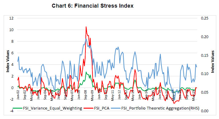 It is evident that the highs in the FSIs could be linked with well-known stress events. All the three FSIs (compiled using different methodologies) peak during the crisis periods of October 2008 relating to the global financial crisis and August 2013 relating to the taper tantrum. In the initial years of 2002-06, moderate US-India 10-year bond spreads and relatively accommodative foreign exchange market conditions and the stable banking sector kept FSI low (except for around May 2004, due to uncertainties around the general election’s results and around March 2006 due to stock market crash following heavy selling by FIIs, retail investors and weaknesses in global markets). FSI witnessed its peak around September/October 2008 reflecting underlying building up of financial stress around the global financial crisis marked by stress in all financial markets that were considered. FSI went up again in December 2011 because of exchange rate pressures. During June and August 2013, following the taper tantrum event, there were exchange rate pressures on account of rupee depreciation due to high net capital outflows. The US Fed’s indication that it may taper off the quantitative easing aggravated stress which got manifested in high FSI values in mid-2013. VI. Financial Stress Index and the real economic activity linkages The relationship between FSI and real economic activity is a complex one. Hakkio and Keeton (2009) observed that increase in financial stress resulted in a decline in economic activities. The relationship between FSI and the real economy, as proxied by IIP growth, was assessed using a correlation analysis and regression method. Though the industry accounts for less than a quarter of GDP, financial stress can be expected to impact IIP growth and its choice to examine real activity linkages is also governed by the better frequency at which this data is available. The lead and lag correlations of these three FSIs with IIP growth indicate that IIP’s correlation with lagged values each of these FSIs was higher than that with lead values of FSIs (Table 2). Further, all the lagged correlations are negative indicating higher values of FSIs are associated with lower IIP growth. Also, the lagged correlation was higher at a lag of 3-months, for each of the FSIs. | Table 2: Cross-correlation of FSI with IIP Growth | | FSI / No. of months | 0 | 1 | 2 | 3 | 4 | 5 | 6 | 7 | 8 | 9 | 10 | 11 | 12 | | FSI_var_eq | Lag | -0.268 | -0.294 | -0.321 | -0.342 | -0.344 | -0.330 | -0.332 | -0.326 | - 0.305 | -0.238 | -0.172 | -0.144 | -0.084 | | Lead | -0.268 | -0.199 | -0.167 | -0.101 | -0.032 | -0.014 | 0.022 | 0.051 | 0.100 | 0.157 | 0.213 | 0.242 | 0.274 | | FSI_PCA | Lag | -0.119 | -0.151 | -0.175 | -0.194 | -0.194 | -0.176 | -0.173 | -0.169 | - 0.149 | -0.092 | -0.036 | -0.013 | 0.041 | | Lead | -0.119 | -0.053 | -0.028 | 0.031 | 0.092 | 0.118 | 0.150 | 0.182 | 0.230 | 0.279 | 0.326 | 0.359 | 0.388 | | FSI_Portfolio_theoretic | Lag | -0.186 | -0.199 | -0.214 | -0.252 | -0.258 | -0.267 | -0.297 | -0.324 | - 0.321 | -0.293 | -0.244 | -0.232 | -0.166 | | Lead | -0.186 | -0.128 | -0.119 | -0.063 | -0.015 | -0.010 | 0.021 | 0.045 | 0.076 | 0.127 | 0.166 | 0.198 | 0.209 | A regression analysis, with IIP growth as the dependent variable, was also used to assess the predictive ability of the FSIs. The base model consists of a lagged dependent variable as the explanatory variable. The base model is then augmented by inclusion of lagged values of each of the three FSIs and the results are furnished under Model 1 to Model 3 in Table 3. The improvement in the adjusted R2 as compared to the base model indicates that each of the FSIs had some predictive power for IIP. Further, the estimated coefficients of the lagged value of each of the FSIs were found to be negative, which is in line with our expectation, and statistically significant, suggesting that the higher the financial stress, the lower the economic activity. | Table 3: Regression Results: Dependent Variable - IIP Growth | | | Base Model | Model 16 | Model 2 | Model 3 | | Constant | 0.65
(0.04) | 0.78
(0.01) | 0.69
(0.03) | 1.99
(0.02) | | IIP_Gr(-1) | 0.51
(0.00) | 0.48
(0.00) | 0.49
(0.00) | 0.50
(0.00) | | IIP_Gr(-2) | 0.37
(0.00) | 0.37
(0.00) | 0.37
(0.00) | 0.36
(0.00) | | FSI_eq_var(-1) | | -0.84
(0.03) | | | | FSI_PCA(-1) | | | -0.18
(0.07) | | | FSI_port(-3)7 | | | | -11.51
(0.08) | | | | Adj. R2 | 0.6693 | 0.6754 | 0.6728 | 0.6718 | | LM test | 1.69
(0.17) | 1.53
(0.21) | 1.49
(0.22) | 1.25
(0.29) | | J-B test | 1.54
(0.46) | 1.98
(0.37) | 1.73
(0.42) | 1.61
(0.45) | | Note: Values in parentheses are the p-values. | VII. Dating the financial crisis episodes For identifying the period of high and low financial stress, this paper uses the method suggested by Duprey et al. (2017). First, months in which the FSIs are above 90 percentile are identified. Then it is seen if these episodes are accompanied with a prolonged decline in real economic activity. Episodes of stress together with ‘six’ consecutive months of real economic stress are considered to be ‘systemic’. Charts 7, 8, and 9 show IIP growth on the y-axis and quantiles of the FSIs on x-axis. As can be seen in the charts that events when the FSIs are above 90th percentile are accompanied by substantial decline in IIP growth. The months when FSIs were above the 90th percentile are identified as June 2008 to May 2009, from September 2011 to January 2012 and from July to September 2013. However, as mentioned earlier, stress is identified to be systemic only when it results in six months of consecutive economic stress (that is negative IIP growth). This systemic period of stress is identified as the third quarter of 2008-09 when the financial crisis took place. VIII. Conclusion The paper is a preliminary foray towards construction of financial stress indicators for the Indian financial system. It uses 11 market-based indicators covering major segments of the Indian financial markets - money market, debt market, equity market, forex market, and the banking sector. Three different methodologies - variance equal weighting, principal component analysis, and portfolio aggregation method were applied to construct the FSIs. All the three FSIs were found to be negatively correlated with real economic activity (IIP growth) and can be used as a leading indicator for predicting the real economic activity. Also, the regression analysis suggested that the FSIs could be helpful in predicting IIP growth. Periods in which FSIs are above 90th percentile also witness substantial decline in IIP growth. While identifying past financial stress, it was seen that systemic stress was present in the Indian financial system during the third quarter of 2008-09.
References Balakrishnan, R., Danninger, S., Elekdag, S., & Tytell, I. (2009). The transmission of financial stress from advanced to emerging economies. IMF Working Paper, 09, 133. Bernanke, B. S., Gertler, M., & Gilchrist, S. (1999). The financial accelerator in a quantitative business cycle framework in J. B. Taylor and M. Woodford (eds.), Handbook of Macroeconomics, 1(3), Amsterdam: North-Holland, 1341-1393. Grimaldi, B. M. (2010). Detecting and interpreting financial stress in the Euro area. ECB Working Paper Series 1214. Cardarelli, R., Elekdag, S., & Lall, S. (2011). Financial stress and economic contractions. Journal of Financial Stability, 7(2), 78-97. Carlson, M. A., Lewis, K. F., & Nelson, W. R. (2012). Using policy intervention to identify financial stress. Finance and Economics Discussion Series 02, Federal Reserve. Cevik, E.I., Dibooglu, S., & Kenc, T. (2013). Measuring financial stress in Turkey. Journal of Policy Modelling, 35 (2), 370-383. Dahalan, J., Abdullah, H. B., & Umar, M. (2016). Measuring financial stress index for Malaysian economy. International Journal of Economics and Financial Issues 6 (3), 942-947. Duprey, T., Benjamin, K., & Peltonen, T. (2017). Dating systemic financial stress episodes in EU countries. Journal of Financial Stability, 32, 30–56 El-Shal, A. (2012). The spillover effects of the global financial crisis on economic activity in emerging economies – investigating the Egyptian case using the financial stress index, Working Papers 737, Economic Research Forum, revised 2012. Gayen, S. (2016). A measure of downside risk in multivariate setup with application in measuring financial stress, Sankhya, B, 78, 287-315. Guru, A. (2016). Early warning system of finance stress for India, International Review of Applied Economics, 30(3), 273-300. Hakkio, C.S., & Keeton, W. R. (2009). Financial stress: what is it, how can it be measured, and why does it matter? Economic Review, 94(2), 5-50. Hanschel, E., & Monnin, P. (2005). Measuring and forecasting stress in the banking sector: evidence from Switzerland. Unpublished Working Paper. BIS papers, 22, 431-449. Hollo, D., Kremer, M., & Lo Duca, M. (2012). CISS-A composite indicator of systemic stress in the financial system. Unpublished Working Paper. ECB Working Paper No. 1426. Huotari, J. (2015). Measuring financial stress – A country specific stress index for Finland. Bank of Finland Research Paper Discussion, 07. Illing, M., & Liu, Y. (2006). Measuring financial stress in a developed country: An application to Canada. Journal of Financial Stability, 2(3), 243-265. Islami, M., & Kurz‐Kim, J. R. (2013). A single composite financial stress indicator and its real impact in the Euro area. International Journal of Finance & Economics, 19(3), 204-211. Johansson, T., & Bonthron, F. (2013). Further development of the index for financial stress for Sweden. Sveriges Riksbank Economic Review, 01. Kliesen,K. L., & Douglas C. Smith (2010). Measuring financial market stress, Economic Synopses, No. 2, Federal Reserve Bank of St. Louis. Kliesen, K. L., Owyang, M. T., & Verman, E. K. (2012). Disentangling diverse measures: A survey of financial stress indexes. Federal Reserve Bank of St. Louis Review, 94(5). Lo Duca, M., & Peltonen, T. A. (2013). Assessing systemic risks and predicting systemic events. Journal of Banking & Finance, 37(7), 2183-2195. Louzis, D. P., & Vouldis A. T. (2013). A financial systemic stress index for Greece. Paper presented at the First Conference of the Macro-prudential Research (MaRs) network of the European System of Central Banks in Frankfurt am Main, October. Monin, Philip J. (2017). The OFR financial stress index. OFR Working Paper, 17(4). Nelson, W. R., & Perli, R. (2007). Selected indicators of financial stability. Irving Fisher Committee's Bulletin on Central Bank Statistics, 23, 92-105. Oet, M. V., Eiben, R., Bianco,T., Gramlich, D., & Ong, S.J. (2012). The financial stress index: identification of systemic risk conditions. Federal Reserve Bank of Cleveland, Working Paper 11-30, November. Park, C. Y. & Mercado R. (2014). Determinants of financial stress in emerging market economies. Journal of Banking & Finance, 45, 199-224. Patel, S. A., & Sarkar, A. (1998). Crises in developed and emerging stock markets. Financial Analysts Journal, 54(6), 50-61. Shankar, A. (2014). A financial conditions index for India. RBI Working Paper Series No.08. Wolken, T. (2013). Measuring systemic risk: the role of macro-prudential indicators, Reserve Bank of New Zealand Bulletin, Reserve Bank of New Zealand. 76, 13-30, December. |