| Press Release RBI Working Paper Series No. 01
Banking Stability - A Precursor to Financial Stability
@Rabi N. Mishra, S. Majumdar and Dimple Bhandia Abstract *This paper focuses on constructing a Banking Stability Map and Indicator and deducing the linkages with the financial markets and macroeconomic variables. In addition, an attempt has been made to establish the direction of causality between stability of the banking sector and overall financial stability. We attempt to answer this question using different dimensions used for the construction of the banking stability indicator. We derive the impact by using VAR framework and Granger’s causality test and also explain the variations through a regression equation. According to the findings, the movements in the banking stability indicator indicate that there are symptoms of a moderate rise in instability of the banking sector in recent periods mainly due to the deterioration in asset quality. The banking sector stress explains a significant portion of variability of stress in the financial market, whereas, explanation of variability of the banking sector stress provided by the financial markets is much less. The impact of GDP growth on the asset quality of the banking sector, assessed using the granger’s causality test, shows that GDP growth significantly impacts the asset quality component of the indicator. Keywords: Banking Stability, Financial Stability, Stability Map, Stability Indicator JEL Classification: C43, G10, G21 I. Introduction The recent financial crisis caused huge cost to the world economies and despite quite substantial research and analysis, there are diverging views about the exact genesis and causes of the crisis. Some of the research analysts have attributed the accommodative monetary policy pursued in the USA during 2003-05 as a major cause of the crisis. Lack of regulatory oversight of non-bank financial intermediaries, ascribed as shadow banking, is considered to be the major cause by another group of analysts. There are also views that the lax lending standards in the sub-prime mortgage markets enabled the continuation and acceleration of the financial crisis. Some of the economists have attributed the financial crisis as a consequence of large global imbalances. Amongst all these diverse opinions and views, there is, however, unanimity that the real act of the financial crisis was enacted in the courtyard of the banking sector where the trigger of financial crisis initially took place. It is perceived that fragile conditions prevailing in the banking sector were allowed to persist for a much longer period.In order to obviate the occurrence of such a crisis in future, there is much emphasis to monitor the broad issues of financial stability including banking sector stability. There are concerted efforts being made by the international organizations, such as IMF, BIS, World Bank, etc. and individual central banks, to evolve various leading indicators of the financial stability, including that of the banking sector, in order to make an informed judgment about the evolving risks to the financial system and initiate corrective policy measures a priori. As banks are the vital components of any financial system, the stability of the banking sector has become a paramount policy initiative worldwide. The issue of financial stability is organically linked with banking stability. In fact the historical evidences demonstrate that those financial crisis which had stronger involvement of the banking sector had more devastating effect on the real sector in terms of fall in real output and reduction in employment level. The financial crisis of 2007-08 was no exception. The theoretical analysis of the events that preceded the financial crisis prove amply that whatsoever may the origin of the financial crisis be, its trigger took place in the banking sector. There are also evidences that the financial crisis persisted for a longer period because of weaknesses in the banking sector which went unnoticed for a longer period. In view of these developments there is an additional emphasis to ensure the stability of the banking sector by strengthening regulatory norms, focusing on empirical research on the leading indicators of banking stability and by preparing banking stability map and banking stability indicator. Banking stability is a yardstick to determine whether an economy is sufficiently strong enough to withstand both the internal and external shocks. On the other side, financial stability is a by-product of stability conditions prevailing in the areas of banking, financial market and the real economy. Out of the three, banking stability conditions emerge as a vital ingredient to financial stability in a country. Banking stability in itself relies on the efficacies of the several parameters of individual banks, e.g., asset quality, liquidity, capital, costs and return on assets, etc. for its degree of stability during the period under review and in the days ahead. Though, the stability of the banking sector gets affected positively or negatively with the conditions prevailing in the financial market and the real economy; ultimately it determines as to what extent financial stability is ensured in the economy by its ability to absorb the shocks. Stability of the banking sector may, therefore, be treated as a forerunner of financial stability in an economy. In view of these developments, in the recent period central banks and other supervisory authorities have started regularly assessing the situation in the banking sector with a focus on how the sector will evolve in the medium term. Initially, the issue of the banking stability was covered under the arena of banking crisis, which was based on the binary variables, signaling whether a banking sector is in crisis or not. But as banking crisis are rare birds, binary variable approach are less suitable to depict the condition of the sector. However, the absence of a full-blown crisis does not mean that the banking sector would continue to be stable in the medium term. In view of the limitations of binary variable oriented models, there have been efforts to develop banking stability indicator through which banking sector stress could be discerned. In fact the advantages banking stability indicator is that it represents a continuum of stability/instability describing the banking sector condition ranging from low level of stability, where the banking sector is in a stage of near crisis, to the high level of stability, when the banking sector is in tranquil. In this background, an attempt has been made, in this paper, to develop a banking stability indicator for India by way of combining some of those indicators which are important in gauging the health of the banking sector. The paper is covered in seven sections. In Section II, we provide a brief on the historical background behind the development of Financial Stability Map & Indicator in India. In Section III we provide methodological aspects of constructing Banking Stability Map and Indicator. Sections IV, V and VI are devoted to analyze the linkage of banking stability indicator with the financial markets and the real sector followed by the broad conclusion and summary of the study in Section VII. References used in the study are given at the end of the paper. II. Historical background behind the development of Financial Stability Map & Indicator in India Globally speaking, many central banks have developed or are in the process of developing various methods to identify risk factors linked with the functioning of their banking and financial markets in order to provide early warning signals to the policymakers to enable them to initiate policy measures a priori. IMF had presented a Global Financial Stability Map (GFSM) in the Global Financial Stability Report (GFSR) of April 2007, and published the methodology in its Working Paper1. GFSM was introduced as a summary tool for communicating changes in the risks and conditions affecting financial stability in a graphical manner. The GFSM coupled with other financial surveillance tools sought to create a more systematic approach towards monitoring the global financial infrastructure and to improve the understanding of risks and conditions that affect financial institutions and other intermediaries. However, it does not consider certain key sources of financial stability risks, for example, operational risks or micro-structure of asset market. Judgment & technical adjustments were important in the final assessment of global financial stability. Judgment is made based on market intelligence and related surveillance work in order to determine the final positioning of risk factors in the Map. Technical adjustment is used to account for numerical limitations of the model. Another attempt by IMF in this direction has been to develop a mechanism called Early Warning Exercise (EWE) jointly with Financial Stability Board (FSB) to detect risks and vulnerabilities that impact financial stability. As part of the exercise, an Early Warning List (EWL) is prepared and for each risk scenario flagged by the EWL, staff of IMF and FSB secretariat identify: a) policy actions to mitigate risks and reduce vulnerabilities; and b) suggestions for further analysis in subsequent EWE rounds. Other central banks have also tried and are still taking steps to develop their own tools and methods to spot risks and vulnerabilities that impact financial stability in their individual countries. One such attempt is the development of a tool entitled “An Index of Financial stress for Canada” by the Bank of Canada. It is a method of deriving an ordinal estimate of macro-economic financial stress in the form of an index. A variety of measures of probable loss, risk and uncertainty are compiled from the banking, foreign exchange, debt and equity markets. Stress in the household sector and the non-financial business sector is implicitly reflected in the behaviour of agents in these four markets which are considered to be the most important channels in Canada. Finally, the conditions prevailing in the financial market segments, viz., debt, equity and foreign exchange exert pressure upon the banking sector; so also real economic parameters like export, import, flow of foreign capital, gross domestic product, etc. determines the volume of banking business. However, ultimately, it is the banking sector that keeps itself resilient against all odds and provides a sense of stability not only to the whole banking & financial system but also to the entire economy of a nation. Against the backdrop of these global developments, initiatives were taken in India as well to develop a mechanism to detect risks and vulnerabilities by way of preparing the Banking Stability Map & Indicator which was published in the December 2010 issue of Financial Stability Report (FSR) of the Reserve Bank of India. The methodology was further enhanced in the subsequent FSRs. III. Constructing Banking Stability Map and Indicator: Methodology The Banking Stability Map and Indicator represent an overall assessment in underlying conditions and inherent risk factors that impact the stability of the banking sector. The Map and Indicator are based on five indices which represent the five dimensions of: - Soundness (S);
- Asset-quality (Q);
- Profitability (P);
- Liquidity (L); and
- Efficiency (E).
A composite measure of each dimension is calculated as a weighted average of a set of standardised ratios (Table 1) which are relevant in assessing the dimension. The ratios are largely drawn from those used by Reserve Bank of India’s supervisory department as part of its CAMELS2 assessment of banks. The weights are also based on the weights assigned to the different ratios for the CAMELS rating. Each index, representing a single dimension of the functioning of the bank’s, takes a values between zero (minimum) and 1 (maximum). The index represents a relative measure for the sample period used for its construction, with a higher value of the index indicating that the risks emanating to the banking sector from that dimension are higher. Therefore, an increase in the value of the index in any particular dimension indicates an increase in risk in that dimension for that period as compared to other periods. The sample period for assessment was taken as March 2001 to March 2012. The ratios used for construction of each composite index are summarised in Table – 1. | Table 1: Ratios used for construction of Banking Stability Map and Indicator | | Dimension | Ratios | | Soundness | CRAR * | Tier_I Capital to Tier_II Capital * | Levarage_ratio as Total-Assets to Capital and Reserves | | Asset-Quality | Net NPAs to Total-Advances | Gross NPAs to Total-Advances | Sub-Standard-advances to gross NPAs * | Restructured-Standard-Advances to Standard-Advances | | Profitability | Return on Assets * | Net Interest Margin * | Growth in Profit * | | Liquidity | Liquid-Assets to Total-Assets * | Customer-Deposits to Total-Assets * | Non-Bank-Advances to Customer-Deposits | Deposits maturing within-1-year to Total Deposits | | Efficiency | Cost to Income
(Operating expenses to income – interest expenses) | Business (Credit + Deposits) to staff expenses * | Staff Expenses to Total Expenses | | * Negatively related with risk | For each of the above ratios, a weighted average for the banking sectors is derived, where the weights are the ratio of individual bank’s asset to the total assets of the banking system. Each index is standardised for the sample period, using a relative distance measure, as (Ratio-on-a-given-date – Minimum-value-in-sample-period)
divided by (Maximum-value-in-sample-period – Minimum-value-in-sample-period) The process of calculation of each ratio (R) is illustrated in Table 2 Table 2: Standardisation of Ratios used for construction of
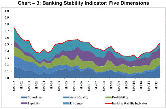
Banking Stability Map and Indicator | | | Assets | Quarter-1 | Quarter-2 | ………. | Quarter-N-1 | Quarter-N | | Bank-1 | A-1 | R(1,1) | R(2,1) | ……….. | R(N-1,1) | R(N,1) | | Bank-2 | A-2 | R(1,2) | R(2,2) | ……….. | R(N-1,2) | R(N,2) | | Bank-3 | A-3 | R(1,3) | R(2,3) | ……….. | R(N-1,3) | R(N,3) | | ---- | ---- | ---- | ---- | ……….. | ---- | ---- | | Bank-M | A-M | R(1,M) | R(2,M) | ……….. | R(N-1,M) | R(N,M) | | Weighted Average by Asset size (WAR) | ∑A * R/ ∑A | ∑A * R/ ∑A | ……….. | ∑A * R/ ∑A | ∑A * R/ ∑A | | Standardised Ratio (SR) | (WAR–min)/ (Max-Min) | (WAR–min)/ (Max-Min) | ……….. | (WAR–min)/ (Max-Min) | (WAR–min)/ (Max-Min) | | Max = Maximum of WAR-1 to WAR-N. Min = Minimum of WAR-1 to WAR-N. | The above calculation is done for each ratio, for getting a standardised ratio, used in the calculation of Banking Stability Map and Indicator. A composite measure of each dimension is calculated as a weighted average of standardised ratios used for that dimension, where the weights are based on the marks assigned for assessment for CAMEL rating. The ratios which are negatively related to risk, one’s complement (1 – SR) is used for calculation of the composite index. Based on the individual composite indices for each dimension, the Banking Stability Indicator (BSI) is constructed as a simple average of the above five composite sub-indices. The higher value of the indicator would suggest lower stability. Generally speaking, the Banking Stability Map (BSM) is a graphical representation of the over-all conditions of the banking sector (Chart - 1), wherein the relative position of the banking sector is presented through three quarter-end points as shown in the Map; pointing to the fact that the risk factors that impact the banking sector have further accentuated during the sample period. This is projected through the BSM which shows a dimensional increase in risk factors emanating from soundness, profitability, liquidity, asset quality and efficiency. Though, the dimension, Soundness showed the relative deterioration vis-a-vis the previous periods, the ratios continue to remain well above the regulatory norms. The Efficiency dimension of the BSM, as derived through cost to income & business per staff expenses ratios, remained more or less at the same level. In the similar fashion, an increase in risk and vulnerability in the banking sector was revealed by the rise in the quarterly series of the BSI beginning with the quarter ended June 2010 (Charts 2 and 3). 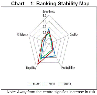 |
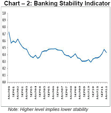 |
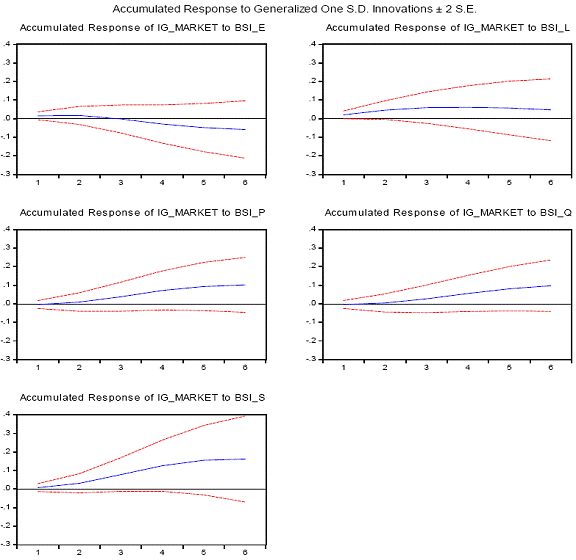
 | The graphical presentation of the BSI reveals that the effect of the global crisis on the Indian banking sector was mild. This is on account of impressive improvement in bank asset quality since the early 2000 on the back of measures taken to clean up banks’ balance sheet, as well as improvements in risk management. As a result, non performing advances (NPAs) declined from a peak of 13 percent of total loans in 2000 to about 2.5 percent in 2011; and the Capital to Risk weighted Assets Ratio (CRAR) steadily improved from 11 percent to 14 percent during the same period. When the current crisis initially hit, it affected mainly banks’ trading books, but these losses were easily absorbed by profits. The second-round effects of the crisis resulted in asset quality deterioration. IV. Interrelationship between the Banking Stability Indicator (BSI) and the Financial Markets Banking is an essential component of the financial markets and thus developments in the banking sector have its ramification on the financial markets. It is presumed that any stress in the banking sector would have impact on markets and vice-a-versa. Therefore, the scope of the analysis is extended to analyze the nature of relationship between BSI and financial markets indicators in a vector autoregression (VAR) framework. A financial markets stability indicator (FMSI) was initially developed following the procedure outlined in the December 2011 issue of the Reserve Bank of India’s FSR. However, on account of non-availability of time series data for all the financial indicators, as included in FMSI, a proxy for it was developed. The proxy reflects the change in market variables considering only three financial market variables, viz. exchange rate, interbank call money rate and equity prices and was named as Index of Growth in Market (IG_Market). It is perceived that during the period of financial turmoil, exchange rate would reveal a tendency of higher depreciation. Similarly during the period of financial instability call rate would increase whereas the equity market would exhibit deceleration. Accordingly we have used annual growth rates (quarter over quarter with-lag-4) of the exchange rate, call rate and BSE equity prices as the indicators of financial stress. The indices have been constructed using the percent ranking method (RBI, FSR, December 2011). The relationship between BSI and IG_Market is examined firstly at the aggregate level and at the second stage between the various components of BSI and IG_Market and these results are discussed below. Aggregate Level The BSI and IG_Market are closely related with correlation coefficient at 0.61. Chart-4 depicts the close movement of BSI and IG_Market. 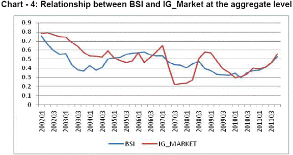 | The relationship was examined using generalized impulse response function of a Vector Autoregressive (VAR) model using BSI and IG_market. It is considered that in case of generalized impulse response function ordering of the variables as in case of Choleski decomposition does not affect the magnitude and direction of response function. The order of the VAR was selected based on minimum information criteria (MIC) and other diagnostics, whereas, stability of the model was judged based on root of characteristic polynomial. Here, all the roots were inside the unit circle which confirms the stability of the VAR system. Also, Jarque-Bera test of normality confirmed that the residuals are multivariate normally distributed. The detailed results are presented in Annex 1. It may be observed from the impulse response function that any stress in the banking sector significantly impacts financial markets adversely, whereas, impact of the market on banking stability in not that significant. Further, variance decomposition analysis shows that the banking stress explains around 33 per cent variability of stress in the financial market, whereas, market explains only 17 per cent of variability of the banking stress. These results intuitively appear to be appropriate as the banking stress is transmitted to the financial markets immediately whereas the impact of financial markets on banking sector takes place with a certain lag. Component Level In order to study the impact of various components of banking stability on the financial markets, a VAR model among the indicators of BSI, viz., soundness, asset-quality, profitability, liquidity and efficiency and the financial market stability indicator (IG_market) has been developed. Based on MIC and other diagnostics, the order of VAR was selected to be 2. The root of characteristic polynomial shows that the VAR system is stable and Jarque-Bera test of normality confirmed that residuals are multivariate normally distributed. The detailed results are given in Annex 2. The dynamics of relationship between stress in the financial market and the components of banking stability indicator was also studied based on generalized impulse response function and variance decomposition. The impulse response function indicated that except for efficiency dimension, the other four components of the banking stability had positive relationship on financial market stability, i.e., any shock in these sectors will adversely impact financial market stability. The variance decomposition of financial market stability indicator indicated that among the five components of BSI, the largest contribution to the variability of financial market stability was from the soundness of the banking system followed by its asset quality. V. Interrelationship between the Banking Stability Indicator and the Real Sector The quality of aggregate asset portfolio of the banking system in a country would depend upon the level of its economic activity. If the economy does not perform well, it will lead to fall in income, business failures and payment difficulties, leading to worsening of asset quality. Hence, GDP growth is expected to be negatively correlated with NPA ratio (Chart-5). The impact of changes in the real economy on the banking sector is expected to be felt through credit growth and asset quality, which finally leads to changes in soundness, profitability, etc. The size of impact of any shock depends upon the level of efficiency, profitability, soundness and liquidity positions of banks. These factors determine the shock absorbing capacity of banks, which finally determine the quantum of feed-back effect the banking system will have on the real economy (Chart-6). 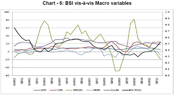 | The relationship between BSI and real sector is examined by estimating a VAR relationship between BSI and the Index of Industrial Production (IIP) and GDP growth, the proxy variables for the health of the real sector. These variables show a relationship with the banking stability indicator through its asset quality component. Improvement in real sector IIP growth or GDP growth tends to improve the banks’ asset quality (BSI-Q) which improves the overall BSI (Annex 3). The trend component of GDP growth and overall BSI, obtained by using HP-filter, also shows a negative relationship with correlation -0.61 (Chart 7). The impact of GDP growth on the asset quality of the banking sector is assessed using the granger’s causality test, which shows that GDP growth impacts the BSI-Q (Quality) (Annex 4). A relationship is also established through a linear regression, which explains about 98 per cent variations in BSI_Q, wherein 88 per cent is explained by its own past and remaining by GDP growth. VI. Shock absorbing capacity of the Banking System BSI_Absorb, constructed as an average of BSI_S, BSI_P and BSI_L, reflects the stability of the banking system from the perspective of its ability to absorb shocks (Chart 8). 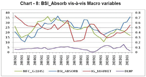 | The relationship between BSR_Absorb with the financial market and the real economy is established through a VAR model (Annex 4). The results shows that the BSI_Absorb (increase in value indicates increase in risk) does influence the market index, though not very significantly, with a lag of two quarters. One per cent positive shock on BSI_Absorb (increase in risk: meaning reduction in shock absorbing capacity) increases the market risk (index) by 0.6 per cent over a period of 3 quarters. The BSI_Absorb also influence the IIP growth, though marginally, as well as the credit growth, through an inverse relationship. One per cent shock on BSI_Absorb reduces the IIP growth by 0.02 per cent over 4 quarters. The impact of BSI_Absorb is significantly higher for credit growth, where one per cent shock on BSI_Absorb brings down the credit growth by 4 per cent over a period of 4 quarters. VII. Broad Summary and Conclusions of the Study In this paper we have established that banking stability is linked with financial stability. Continued financial stability improves banking stability and enables the banking sector to absorb the shocks during times of crises, thus minimizing the impact and helping the economy to bounce back with minimum time lag. The good health of the real economy helps to build soundness, efficiency and profitability of banking system. The impact of shocks in the real economy is reflected on the banking sector through reduced credit growth and deterioration in asset quality. The quantum of feed-back impact from banking sector to the real sector is determined by the level of shock absorbing capacity of the banking sector. This paper is devoted to the issue of developing a banking stability indicator for India. The banking stability indicator is based on five parameters which provide insight into the banks’ performance and thus could be in a way considered leading indicators of the nature of developments likely to occur in the banking sector as a whole. The movements in the banking stability indicator amply capture the profile of the Indian banks and indicate that there are symptoms of a moderate rise in instability of the banking sector in recent periods perhaps due to the rise in the NPA. Thus there is a need to exert precautionary measures to improve the overall performance of the banking sector and initiate regulatory measures appropriately. It may however be clarified that banking stability indicator is presently placed at 0.52 as compared to the 0.75 in 2001-02. The empirical results of this paper indicate that banking instability has immediate adverse effect on the financial markets stability as well as real sector output, whereas the impact of financial market instability and real sector inefficiencies on the banking sector occurs with a certain lag. This analysis in fact provides supporting evidences that the banking stability indicator, as developed in this paper, captures the nuances of the banking sector. These results also indicate that stability in the banking sector is a necessary condition for maintaining financial stability. The paper also indicates that real sector stability, judged in terms of high growth rate, and banking sector stability are intervened. Deterioration in the banking stability indicator has adverse impact on the real sector and similarly deceleration in the real sector performance will adversely affect banking sector. These results in fact have very significant policy implications. Policy makers will need to work towards strengthening the banking sector to enable the banks to bear the shocks resulting from an adverse turn in the real sector environment. There is a need to build enough safeguard in the banking sector to avoid the negative feed-back loop between the banking sector and the real sector which could lead to the germination and aggravation of a financial crisis.
References Basel Committee on Banking Supervision (2011), ‘The Transmission Channels Between The Financial And Real Sectors: A Critical Survey of the Literature’, Working Paper No. 18, BIS Blaise Gadanecz and Kaushik Jayaram (2009). Measures of financial stability – a review. BIS, IFC Bulletin No 31. Claudiu Tiberiu ALBULESCU (2010). Forecasting the Romanian financial system stability using a stochastic simulation model. Romanian Journal of Economic Forecasting – 1. Elsinger, H, Lehar, A and Summer, M (2002), ‘Risk assessment for banking systems’, Oestereichische Nationalbank Working Paper no. 79. Garry J. Schinasi, (2004), ‘Defining Financial Stability’, IMF Working Paper No. WP/04/187 IMF (2009). Global Financial Stability Report, April 2009. Reserve Bank of India. Financial Stability Report – December 2011. Reserve Bank of India. Financial Stability Report – June 2011. Verlis C. Morris (2010). Measuring and Forecasting Financial Stability: The Composition of an Aggregate Financial Stability Index for Jamaica. Bank of Jamaica, August 2010.
Annex 1
Financial Market vis-à-vis banking stability: at Aggregate level
| VAR Residual Serial Correlation LM Tests | | Null Hypothesis: no serial correlation at lag order h | | Lags | LM-Stat | Prob | | 1 | 6.611290 | 0.1579 | | 2 | 1.448345 | 0.8358 | | 3 | 4.789246 | 0.3096 | | 4 | 7.734305 | 0.1018 | | 5 | 4.250260 | 0.3732 | | 6 | 6.186062 | 0.1857 | | 7 | 1.676196 | 0.7950 | | 8 | 3.166747 | 0.5303 | | Probs from chi-square with 4 df. |
| VAR Residual Normality Tests | | Orthogonalization: Cholesky (Lutkepohl) | | Null Hypothesis: residuals are multivariate normal | | Component | Jarque-Bera | df | Prob. | | 1 | 0.060841 | 2 | 0.9700 | | 2 | 9.823136 | 2 | 0.0074 | | Joint | 9.883977 | 4 | 0.0424 |
| Variance Decomposition of BSI: | | Period | S.E. | BSI | IG_MARKET | | 1 | 0.040981 | 100.0000 | 0.000000 | | 2 | 0.053409 | 98.65099 | 1.349009 | | 3 | 0.060653 | 96.28726 | 3.712738 | | 4 | 0.065271 | 93.54920 | 6.450801 | | 5 | 0.068313 | 90.87105 | 9.128952 | | 6 | 0.070335 | 88.50477 | 11.49523 | | 7 | 0.071676 | 86.56289 | 13.43711 | | 8 | 0.072556 | 85.06281 | 14.93719 | | 9 | 0.073127 | 83.96470 | 16.03530 | | 10 | 0.073491 | 83.20075 | 16.79925 |
| Variance Decomposition of IG_MARKET: | | Period | S.E. | BSI | IG_MARKET | | 1 | 0.074115 | 10.12293 | 89.87707 | | 2 | 0.093958 | 14.77030 | 85.22970 | | 3 | 0.104258 | 19.33550 | 80.66450 | | 4 | 0.110188 | 23.40982 | 76.59018 | | 5 | 0.113816 | 26.75841 | 73.24159 | | 6 | 0.116142 | 29.31447 | 70.68553 | | 7 | 0.117692 | 31.13568 | 68.86432 | | 8 | 0.118753 | 32.34857 | 67.65143 | | 9 | 0.119493 | 33.10104 | 66.89896 | | 10 | 0.120011 | 33.53114 | 66.46886 | | Cholesky Ordering: BSI IG_MARKET |
Annex 2
Financial Market vis-à-vis banking stability: at component level Stability of the VAR System
| VAR Residual Serial Correlation LM Tests | | Null Hypothesis: no serial correlation at lag order h | | Lags | LM-Stat | Prob | | 1 | 36.92269 | 0.4261 | | 2 | 35.30342 | 0.5015 | | 3 | 43.39866 | 0.1852 | | 4 | 48.72298 | 0.0765 | | 5 | 31.72192 | 0.6723 | | 6 | 42.93559 | 0.1983 | | 7 | 29.63929 | 0.7640 | | 8 | 25.04325 | 0.9148 | | Probs from chi-square with 36 df. |
| VAR Residual Normality Tests | | Orthogonalization: Cholesky (Lutkepohl) | | Null Hypothesis: residuals are multivariate normal | | Component | Skewness | Chi-sq | df | Prob. | | 1 | -0.345250 | 0.754920 | 1 | 0.3849 | | 2 | -0.388968 | 0.958210 | 1 | 0.3276 | | 3 | 0.275963 | 0.482319 | 1 | 0.4874 | | 4 | -0.032152 | 0.006547 | 1 | 0.9355 | | 5 | 0.351307 | 0.781640 | 1 | 0.3766 | | 6 | 0.045860 | 0.013320 | 1 | 0.9081 | | Joint | | 2.996956 | 6 | 0.8092 | | Component | Kurtosis | Chi-sq | df | Prob. | | 1 | 3.172241 | 0.046973 | 1 | 0.8284 | | 2 | 2.502089 | 0.392533 | 1 | 0.5310 | | 3 | 3.071077 | 0.007999 | 1 | 0.9287 | | 4 | 3.726349 | 0.835339 | 1 | 0.3607 | | 5 | 2.968510 | 0.001570 | 1 | 0.9684 | | 6 | 2.913766 | 0.011774 | 1 | 0.9136 | | Joint | | 1.296187 | 6 | 0.9719 | | Component | Jarque-Bera | df | Prob. | | | 1 | 0.801892 | 2 | 0.6697 | | | 2 | 1.350742 | 2 | 0.5090 | | | 3 | 0.490318 | 2 | 0.7826 | | | 4 | 0.841886 | 2 | 0.6564 | | | 5 | 0.783210 | 2 | 0.6760 | | | 6 | 0.025094 | 2 | 0.9875 | | | Joint | 4.293142 | 12 | 0.9775 | |
 |
| Variance Decomposition of IG_Market | | Period | S.E. | BSI_E | BSI_L | BSI_P | BSI_Q | BSI_S | G_MARKET | | 1 | 0.118877 | 5.085286 | 5.743797 | 0.678703 | 1.365436 | 0.005420 | 87.12136 | | 2 | 0.147548 | 2.417306 | 10.13555 | 4.085811 | 5.761436 | 1.177991 | 76.42190 | | 3 | 0.156589 | 4.368396 | 10.20505 | 7.286308 | 9.760558 | 10.94706 | 57.43263 | | 4 | 0.166695 | 7.562291 | 8.655580 | 9.091696 | 12.47199 | 18.13482 | 44.08362 | | 5 | 0.174683 | 8.655991 | 7.767322 | 9.143977 | 14.13123 | 20.15863 | 40.14285 | | 6 | 0.178522 | 8.945060 | 7.794431 | 8.939894 | 14.54607 | 19.92863 | 39.84592 | | Cholesky Ordering: BSI_E BSI_L BSI_P BSI_Q BSI_S IG_MARKET |
Annex 3
Real Economy vis-à-vis banking stability: at Aggregate level
| Pairwise Granger Causality Tests | | Sample: 2002Q1 2011Q4 | | Lags: 2 | | Null Hypothesis: | Obs | F-Statistic | Prob. | | GDP_CN_G does not Granger Cause BSI_Q | 38 | 9.94181 | 0.0004 | | BSI_Q does not Granger Cause GDP_CN_G | | 0.75709 | 0.4770 |
| Dependent Variable: BSI_Q | | Method: Least Squares | | Sample (adjusted): 2002Q3 2011Q4 | | Included observations: 38 after adjustments | | Variable | Coefficient | Std. Error | t-Statistic | Prob. | | C | 0.079814 | 0.027930 | 2.857643 | 0.0071 | | BSI_Q(-1) | 0.880335 | 0.025000 | 35.21387 | 0.0000 | | GDP_CN_G(-2) | -0.007950 | 0.002890 | -2.750851 | 0.0093 | | R-squared | 0.983354 | Mean dependent var | 0.255605 | | Adjusted R-squared | 0.982403 | S.D. dependent var | 0.210736 | | S.E. of regression | 0.027955 | Akaike info criterion | -4.240788 | | Sum squared resid | 0.027352 | Schwarz criterion | -4.111505 | | Log likelihood | 83.57497 | Hannan-Quinn criter. | -4.194790 | | F-statistic | 1033.815 | Durbin-Watson stat | 2.032653 | | Prob(F-statistic) | 0.000000 | |
Annex 4 Banking systems’ shock absorbing capacity vis-s-vis Real Economy and
Financial Markets: at Aggregate level BSI_Absorb and Financial Market BSI_Absorb and Real Economy |